Programming


This is part 8 of Categories for Programmers. Previously: Functors. See the Table of Contents.

Now that you know what a functor is, and have seen a few examples, let’s see how we can build larger functors from smaller ones. In particular it’s interesting to see which type constructors (which correspond to mappings between objects in a category) can be extended to functors (which include mappings between morphisms).

Bifunctors

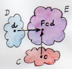
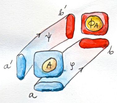
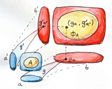
Since functors are morphisms in Cat (the category of categories), a lot of intuitions about morphisms — and functions in particular — apply to functors as well. For instance, just like you can have a function of two arguments, you can have a functor of two arguments, or a bifunctor. On objects, a bifunctor maps every pair of objects, one from category C, and one from category D, to an object in category E. Notice that this is just saying that it’s a mapping from a cartesian product of categories C×D to E.

Bifunctor

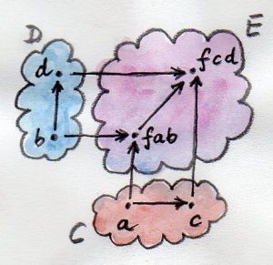
That’s pretty straightforward. But functoriality means that a bifunctor has to map morphisms as well. This time, though, it must map a pair of morphisms, one from C and one from D, to a morphism in E.

Again, a pair of morphisms is just a single morphism in the product category C×D. We define a morphism in a cartesian product of categories as a pair of morphisms which goes from one pair of objects to another pair of objects. These pairs of morphisms can be composed in the obvious way:

(f, g) ∘ (f', g') = (f ∘ f', g ∘ g')

The composition is associative and it has an identity — a pair of identity morphisms (id, id). So a cartesian product of categories is indeed a category.

An easier way to think about bifunctors would be to consider them functors in each argument separately. So instead of translating functorial laws — associativity and identity preservation — from functors to bifunctors, it would be enough to check them separately for each argument. However, in general, separate functoriality is not enough to prove joint functoriality. Categories in which joint functoriality fails are called premonoidal.

Let’s define a bifunctor in Haskell. In this case all three categories are the same: the category of Haskell types. A bifunctor is a type constructor that takes two type arguments. Here’s the definition of the Bifunctor typeclass taken directly from the library Control.Bifunctor:

class Bifunctor f where
    bimap :: (a -> c) -> (b -> d) -> f a b -> f c d
    bimap g h = first g . second h
    first :: (a -> c) -> f a b -> f c b
    first g = bimap g id
    second :: (b -> d) -> f a b -> f a d
    second = bimap id

The type variable f represents the bifunctor. You can see that in all type signatures it’s always applied to two type arguments. The first type signature defines bimap: a mapping of two functions at once. The result is a lifted function, (f a b -> f c d), operating on types generated by the bifunctor’s type constructor. There is a default implementation of bimap in terms of first and second, which shows that it’s enough to have functoriality in each argument separately to be able to define a bifunctor. (As mentioned before, this doesn’t always work, because the two maps may not commute, that is first g . second h may not be the same as second h . first g.)

Bimap

bimap

The two other type signatures, first and second, are the two fmaps witnessing the functoriality of f in the first and the second argument, respectively.

First

first

Second

second

The typeclass definition provides default implementations for both of them in terms of bimap.

When declaring an instance of Bifunctor, you have a choice of either implementing bimap and accepting the defaults for first and second, or implementing both first and second and accepting the default for bimap (of course, you may implement all three of them, but then it’s up to you to make sure they are related to each other in this manner).

Product and Coproduct Bifunctors

An important example of a bifunctor is the categorical product — a product of two objects that is defined by a universal construction. If the product exists for any pair of objects, the mapping from those objects to the product is bifunctorial. This is true in general, and in Haskell in particular. Here’s the Bifunctor instance for a pair constructor — the simplest product type:

instance Bifunctor (,) where
    bimap f g (x, y) = (f x, g y)

There isn’t much choice: bimap simply applies the first function to the first component, and the second function to the second component of a pair. The code pretty much writes itself, given the types:

bimap :: (a -> c) -> (b -> d) -> (a, b) -> (c, d)

The action of the bifunctor here is to make pairs of types, for instance:

(,) a b = (a, b)

By duality, a coproduct, if it’s defined for every pair of objects in a category, is also a bifunctor. In Haskell, this is exemplified by the Either type constructor being an instance of Bifunctor:

instance Bifunctor Either where
    bimap f _ (Left x)  = Left (f x)
    bimap _ g (Right y) = Right (g y)

This code also writes itself.

Now, remember when we talked about monoidal categories? A monoidal category defines a binary operator acting on objects, together with a unit object. I mentioned that Set is a monoidal category with respect to cartesian product, with the singleton set as a unit. And it’s also a monoidal category with respect to disjoint union, with the empty set as a unit. What I haven’t mentioned is that one of the requirements for a monoidal category is that the binary operator be a bifunctor. This is a very important requirement — we want the monoidal product to be compatible with the structure of the category, which is defined by morphisms. We are now one step closer to the full definition of a monoidal category (we still need to learn about naturality, before we can get there).

Functorial Algebraic Data Types

We’ve seen several examples of parameterized data types that turned out to be functors — we were able to define fmap for them. Complex data types are constructed from simpler data types. In particular, algebraic data types (ADTs) are created using sums and products. We have just seen that sums and products are functorial. We also know that functors compose. So if we can show that the basic building blocks of ADTs are functorial, we’ll know that parameterized ADTs are functorial too.

So what are the building blocks of parameterized algebraic data types? First, there are the items that have no dependency on the type parameter of the functor, like Nothing in Maybe, or Nil in List. They are equivalent to the Const functor. Remember, the Const functor ignores its type parameter (really, the second type parameter, which is the one of interest to us, the first one being kept constant).

Then there are the elements that simply encapsulate the type parameter itself, like Just in Maybe. They are equivalent to the identity functor. I mentioned the identity functor previously, as the identity morphism in Cat, but didn’t give its definition in Haskell. Here it is:

data Identity a = Identity a
instance Functor Identity where
    fmap f (Identity x) = Identity (f x)

You can think of Identity as the simplest possible container that always stores just one (immutable) value of type a.

Everything else in algebraic data structures is constructed from these two primitives using products and sums.

With this new knowledge, let’s have a fresh look at the Maybe type constructor:

data Maybe a = Nothing | Just a

It’s a sum of two types, and we now know that the sum is functorial. The first part, Nothing can be represented as a Const () acting on a (the first type parameter of Const is set to unit — later we’ll see more interesting uses of Const). The second part is just a different name for the identity functor. We could have defined Maybe, up to isomorphism, as:

type Maybe a = Either (Const () a) (Identity a)

So Maybe is the composition of the bifunctor Either with two functors, Const () and Identity. (Const is really a bifunctor, but here we always use it partially applied.)

We’ve already seen that a composition of functors is a functor — we can easily convince ourselves that the same is true of bifunctors. All we need is to figure out how a composition of a bifunctor with two functors works on morphisms. Given two morphisms, we simply lift one with one functor and the other with the other functor. We then lift the resulting pair of lifted morphisms with the bifunctor.

We can express this composition in Haskell. Let’s define a data type that is parameterized by a bifunctor bf (it’s a type variable that is a type constructor that takes two types as arguments), two functors fu and gu (type constructors that take one type variable each), and two regular types a and b. We apply fu to a and gu to b, and then apply bf to the resulting two types:

newtype BiComp bf fu gu a b = BiComp (bf (fu a) (gu b))

That’s the composition on objects, or types. Notice how in Haskell we apply type constructors to types, just like we apply functions to arguments. The syntax is the same.

If you’re getting a little lost, try applying BiComp to Either, Const (), Identity, a, and b, in this order. You will recover our bare-bone version of Maybe b (a is ignored).

The new data type BiComp is a bifunctor in a and b, but only if bf is itself a Bifunctor and fu and gu are Functors. The compiler must know that there will be a definition of bimap available for bf, and definitions of fmap for fu and gu. In Haskell, this is expressed as a precondition in the instance declaration: a set of class constraints followed by a double arrow:

instance (Bifunctor bf, Functor fu, Functor gu) =>
  Bifunctor (BiComp bf fu gu) where
    bimap f1 f2 (BiComp x) = BiComp ((bimap (fmap f1) (fmap f2)) x)

The implementation of bimap for BiComp is given in terms of bimap for bf and the two fmaps for fu and gu. The compiler automatically infers all the types and picks the correct overloaded functions whenever BiComp is used.

The x in the definition of bimap has the type:

bf (fu a) (gu b)

which is quite a mouthful. The outer bimap breaks through the outer bf layer, and the two fmaps dig under fu and gu, respectively. If the types of f1 and f2 are:

f1 :: a -> a'
f2 :: b -> b'

then the final result is of the type bf (fu a') (gu b'):

bimapbf :: (fu a -> fu a') -> (gu b -> gu b') 
  -> bf (fu a) (gu b) -> bf (fu a') (gu b')

If you like jigsaw puzzles, these kinds of type manipulations can provide hours of entertainment.

So it turns out that we didn’t have to prove that Maybe was a functor — this fact followed from the way it was constructed as a sum of two functorial primitives.

A perceptive reader might ask the question: If the derivation of the Functor instance for algebraic data types is so mechanical, can’t it be automated and performed by the compiler? Indeed, it can, and it is. You need to enable a particular Haskell extension by including this line at the top of your source file:

{-# LANGUAGE DeriveFunctor #-}

and then add deriving Functor to your data structure:

data Maybe a = Nothing | Just a
  deriving Functor

and the corresponding fmap will be implemented for you.

The regularity of algebraic data structures makes it possible to derive instances not only of Functor but of several other type classes, including the Eq type class I mentioned before. There is also the option of teaching the compiler to derive instances of your own typeclasses, but that’s a bit more advanced. The idea though is the same: You provide the behavior for the basic building blocks and sums and products, and let the compiler figure out the rest.

Functors in C++

If you are a C++ programmer, you obviously are on your own as far as implementing functors goes. However, you should be able to recognize some types of algebraic data structures in C++. If such a data structure is made into a generic template, you should be able to quickly implement fmap for it.

Let’s have a look at a tree data structure, which we would define in Haskell as a recursive sum type:

data Tree a = Leaf a | Node (Tree a) (Tree a)
    deriving Functor

As I mentioned before, one way of implementing sum types in C++ is through class hierarchies. It would be natural, in an object-oriented language, to implement fmap as a virtual function of the base class Functor and then override it in all subclasses. Unfortunately this is impossible because fmap is a template, parameterized not only by the type of the object it’s acting upon (the this pointer) but also by the return type of the function that’s been applied to it. Virtual functions cannot be templatized in C++. We’ll implement fmap as a generic free function, and we’ll replace pattern matching with dynamic_cast.

The base class must define at least one virtual function in order to support dynamic casting, so we’ll make the destructor virtual (which is a good idea in any case):

template<class T>
struct Tree {
    virtual ~Tree() {};
};

The Leaf is just an Identity functor in disguise:

template<class T>
struct Leaf : public Tree<T> {
    T _label;
    Leaf(T l) : _label(l) {}
};

The Node is a product type:

template<class T>
struct Node : public Tree<T> {
    Tree<T> * _left;
    Tree<T> * _right;
    Node(Tree<T> * l, Tree<T> * r) : _left(l), _right(r) {}
};

When implementing fmap we take advantage of dynamic dispatching on the type of the Tree. The Leaf case applies the Identity version of fmap, and the Node case is treated like a bifunctor composed with two copies of the Tree functor. As a C++ programmer, you’re probably not used to analyzing code in these terms, but it’s a good exercise in categorical thinking.

template<class A, class B>
Tree<B> * fmap(std::function<B(A)> f, Tree<A> * t)
{
    Leaf<A> * pl = dynamic_cast <Leaf<A>*>(t);
    if (pl)
        return new Leaf<B>(f (pl->_label));
    Node<A> * pn = dynamic_cast<Node<A>*>(t);
    if (pn)
        return new Node<B>( fmap<A>(f, pn->_left)
                          , fmap<A>(f, pn->_right));
    return nullptr;
}

For simplicity, I decided to ignore memory and resource management issues, but in production code you would probably use smart pointers (unique or shared, depending on your policy).

Compare it with the Haskell implementation of fmap:

instance Functor Tree where
    fmap f (Leaf a) = Leaf (f a)
    fmap f (Node t t') = Node (fmap f t) (fmap f t')

This implementation can also be automatically derived by the compiler.

The Writer Functor

I promised that I would come back to the Kleisli category I described earlier. Morphisms in that category were represented as “embellished” functions returning the Writer data structure.

type Writer a = (a, String)

I said that the embellishment was somehow related to endofunctors. And, indeed, the Writer type constructor is functorial in a. We don’t even have to implement fmap for it, because it’s just a simple product type.

But what’s the relation between a Kleisli category and a functor — in general? A Kleisli category, being a category, defines composition and identity. Let’ me remind you that the composition is given by the fish operator:

(>=>) :: (a -> Writer b) -> (b -> Writer c) -> (a -> Writer c)
m1 >=> m2 = \x -> 
    let (y, s1) = m1 x
        (z, s2) = m2 y
    in (z, s1 ++ s2)

and the identity morphism by a function called return:

return :: a -> Writer a
return x = (x, "")

It turns out that, if you look at the types of these two functions long enough (and I mean, long enough), you can find a way to combine them to produce a function with the right type signature to serve as fmap. Like this:

fmap f = id >=> (\x -> return (f x))

Here, the fish operator combines two functions: one of them is the familiar id, and the other is a lambda that applies return to the result of acting with f on the lambda’s argument. The hardest part to wrap your brain around is probably the use of id. Isn’t the argument to the fish operator supposed to be a function that takes a “normal” type and returns an embellished type? Well, not really. Nobody says that a in a -> Writer b must be a “normal” type. It’s a type variable, so it can be anything, in particular it can be an embellished type, like Writer b.

So id will take Writer a and turn it into Writer a. The fish operator will fish out the value of a and pass it as x to the lambda. There, f will turn it into a b and return will embellish it, making it Writer b. Putting it all together, we end up with a function that takes Writer a and returns Writer b, exactly what fmap is supposed to produce.

Notice that this argument is very general: you can replace Writer with any type constructor. As long as it supports a fish operator and return, you can define fmap as well. So the embellishment in the Kleisli category is always a functor. (Not every functor, though, gives rise to a Kleisli category.)

You might wonder if the fmap we have just defined is the same fmap the compiler would have derived for us with deriving Functor. Interestingly enough, it is. This is due to the way Haskell implements polymorphic functions. It’s called parametric polymorphism, and it’s a source of so called theorems for free. One of those theorems says that, if there is an implementation of fmap for a given type constructor, one that preserves identity, then it must be unique.

Covariant and Contravariant Functors

Now that we’ve reviewed the writer functor, let’s go back to the reader functor. It was based on the partially applied function-arrow type constructor:

(->) r

We can rewrite it as a type synonym:

type Reader r a = r -> a

for which the Functor instance, as we’ve seen before, reads:

instance Functor (Reader r) where
    fmap f g = f . g

But just like the pair type constructor, or the Either type constructor, the function type constructor takes two type arguments. The pair and Either were functorial in both arguments — they were bifunctors. Is the function constructor a bifunctor too?

Let’s try to make it functorial in the first argument. We’ll start with a type synonym — it’s just like the Reader but with the arguments flipped:

type Op r a = a -> r

This time we fix the return type, r, and vary the argument type, a. Let’s see if we can somehow match the types in order to implement fmap, which would have the following type signature:

fmap :: (a -> b) -> (a -> r) -> (b -> r)

With just two functions taking a and returning, respectively, b and r, there is simply no way to build a function taking b and returning r! It would be different if we could somehow invert the first function, so that it took b and returned a instead. We can’t invert an arbitrary function, but we can go to the opposite category.

A short recap: For every category C there is a dual category Cop. It’s a category with the same objects as C, but with all the arrows reversed.

Consider a functor that goes between Cop and some other category D:
F :: Cop → D
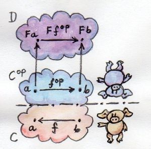
Such a functor maps a morphism fop :: a → b in Cop to the morphism F fop :: F a → F b in D. But the morphism fop secretly corresponds to some morphism f :: b → a in the original category C. Notice the inversion.

Now, F is a regular functor, but there is another mapping we can define based on F, which is not a functor — let’s call it G. It’s a mapping from C to D. It maps objects the same way F does, but when it comes to mapping morphisms, it reverses them. It takes a morphism f :: b → a in C, maps it first to the opposite morphism fop :: a → b and then uses the functor F on it, to get F fop :: F a → F b.

Contravariant

Considering that F a is the same as G a and F b is the same as G b, the whole trip can be described as:
G f :: (b → a) → (G a → G b)
It’s a “functor with a twist.” A mapping of categories that inverts the direction of morphisms in this manner is called a contravariant functor. Notice that a contravariant functor is just a regular functor from the opposite category. The regular functors, by the way — the kind we’ve been studying thus far — are called covariant functors.

Here’s the typeclass defining a contravariant functor (really, a contravariant endofunctor) in Haskell:

class Contravariant f where
    contramap :: (b -> a) -> (f a -> f b)

Our type constructor Op is an instance of it:

instance Contravariant (Op r) where
    -- (b -> a) -> Op r a -> Op r b
    contramap f g = g . f

Notice that the function f inserts itself before (that is, to the right of) the contents of Op — the function g.

The definition of contramap for Op may be made even terser, if you notice that it’s just the function composition operator with the arguments flipped. There is a special function for flipping arguments, called flip:

flip :: (a -> b -> c) -> (b -> a -> c)
flip f y x = f x y

With it, we get:

contramap = flip (.)

Profunctors

We’ve seen that the function-arrow operator is contravariant in its first argument and covariant in the second. Is there a name for such a beast? It turns out that, if the target category is Set, such a beast is called a profunctor. Because a contravariant functor is equivalent to a covariant functor from the opposite category, a profunctor is defined as:
Cop × D → Set

Since, to first approximation, Haskell types are sets, we apply the name Profunctor to a type constructor p of two arguments, which is contra-functorial in the first argument and functorial in the second. Here’s the appropriate typeclass taken from the Data.Profunctor library:

class Profunctor p where
  dimap :: (a -> b) -> (c -> d) -> p b c -> p a d
  dimap f g = lmap f . rmap g
  lmap :: (a -> b) -> p b c -> p a c
  lmap f = dimap f id
  rmap :: (b -> c) -> p a b -> p a c
  rmap = dimap id

All three functions come with default implementations. Just like with Bifunctor, when declaring an instance of Profunctor, you have a choice of either implementing dimap and accepting the defaults for lmap and rmap, or implementing both lmap and rmap and accepting the default for dimap.

dimap

dimap

Now we can assert that the function-arrow operator is an instance of a Profunctor:

instance Profunctor (->) where
  dimap ab cd bc = cd . bc . ab
  lmap = flip (.)
  rmap = (.)

Profunctors have their application in the Haskell lens library. We’ll see them again when we talk about ends and coends.

The Hom-Functor

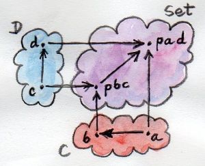
The above examples are the reflection of a more general statement that the mapping that takes a pair of objects a and b and assigns to it the set of morphisms between them, the hom-set C(a, b), is a functor. It is a functor from the product category Cop×C to the category of sets, Set.

Let’s define its action on morphisms. A morphism in Cop×C is a pair of morphisms from C:

f :: a'→ a
g :: b → b'

The lifting of this pair must be a morphism (a function) from the set C(a, b) to the set C(a', b'). Just pick any element h of C(a, b) (it’s a morphism from a to b) and assign to it:

g ∘ h ∘ f

which is an element of C(a', b').

As you can see, the hom-functor is a special case of a profunctor.

Challenges

  1. Show that the data type:
    data Pair a b = Pair a b

    is a bifunctor. For additional credit implement all three methods of Bifunctor and use equational reasoning to show that these definitions are compatible with the default implementations whenever they can be applied.

  2. Show the isomorphism between the standard definition of Maybe and this desugaring:
    type Maybe' a = Either (Const () a) (Identity a)

    Hint: Define two mappings between the two implementations. For additional credit, show that they are the inverse of each other using equational reasoning.

  3. Let’s try another data structure. I call it a PreList because it’s a precursor to a List. It replaces recursion with a type parameter b.
    data PreList a b = Nil | Cons a b

    You could recover our earlier definition of a List by recursively applying PreList to itself (we’ll see how it’s done when we talk about fixed points).

    Show that PreList is an instance of Bifunctor.

  4. Show that the following data types define bifunctors in a and b:
    data K2 c a b = K2 c
    data Fst a b = Fst a
    data Snd a b = Snd b

    For additional credit, check your solutions agains Conor McBride’s paper Clowns to the Left of me, Jokers to the Right.

  5. Define a bifunctor in a language other than Haskell. Implement bimap for a generic pair in that language.
  6. Should std::map be considered a bifunctor or a profunctor in the two template arguments Key and T? How would you redesign this data type to make it so?

Next: Function Types.

Acknowledgment

As usual, big thanks go to Gershom Bazerman for reviewing this article.


In the previous instalment of Category Theory for Programmers we talked about the category of types and functions. If you’re new to the series, here’s the Table of Contents.

You can get real appreciation for categories by studying a variety of examples. Categories come in all shapes and sizes and often pop up in unexpected places. We’ll start with something really simple.

No Objects

The most trivial category is one with zero objects and, consequently, zero morphisms. It’s a very sad category by itself, but it may be important in the context of other categories, for instance, in the category of all categories (yes, there is one). If you think that an empty set makes sense, then why not an empty category?

Simple Graphs

You can build categories just by connecting objects with arrows. You can imagine starting with any directed graph and making it into a category by simply adding more arrows. First, add an identity arrow at each node. Then, for any two arrows such that the end of one coincides with the beginning of the other (in other words, any two composable arrows), add a new arrow to serve as their composition. Every time you add a new arrow, you have to also consider its composition with any other arrow (except for the identity arrows) and itself. You usually end up with infinitely many arrows, but that’s okay.

Another way of looking at this process is that you’re creating a category, which has an object for every node in the graph, and all possible chains of composable graph edges as morphisms. (You may even consider identity morphisms as special cases of chains of length zero.)

Such a category is called a free category generated by a given graph. It’s an example of a free construction, a process of completing a given structure by extending it with a minimum number of items to satisfy its laws (here, the laws of a category). We’ll see more examples of it in the future.

Orders

And now for something completely different! A category where a morphism is a relation between objects: the relation of being less than or equal. Let’s check if it indeed is a category. Do we have identity morphisms? Every object is less than or equal to itself: check! Do we have composition? If a <= b and b <= c then a <= c: check! Is composition associative? Check! A set with a relation like this is called a preorder, so a preorder is indeed a category.

You can also have a stronger relation, that satisfies an additional condition that, if a <= b and b <= a then a must be the same as b. That’s called a partial order.

Finally, you can impose the condition that any two objects are in a relation with each other, one way or another; and that gives you a linear order or total order.

Let’s characterize these ordered sets as categories. A preorder is a category where there is at most one morphism going from any object a to any object b. Another name for such a category is “thin.” A preorder is a thin category.

A set of morphisms from object a to object b in a category C is called a hom-set and is written as C(a, b) (or, sometimes, HomC(a, b)). So every hom-set in a preorder is either empty or a singleton. That includes the hom-set C(a, a), the set of morphisms from a to a, which must be a singleton, containing only the identity, in any preorder. You may, however, have cycles in a preorder. Cycles are forbidden in a partial order.

It’s very important to be able to recognize preorders, partial orders, and total orders because of sorting. Sorting algorithms, such as quicksort, bubble sort, merge sort, etc., can only work correctly on total orders. Partial orders can be sorted using topological sort.

Monoid as Set

Monoid is an embarrassingly simple but amazingly powerful concept. It’s the concept behind basic arithmetics: Both addition and multiplication form a monoid. Monoids are ubiquitous in programming. They show up as strings, lists, foldable data structures, futures in concurrent programming, events in functional reactive programming, and so on.

Traditionally, a monoid is defined as a set with a binary operation. All that’s required from this operation is that it’s associative, and that there is one special element that behaves like a unit with respect to it.

For instance, natural numbers with zero form a monoid under addition. Associativity means that:

(a + b) + c = a + (b + c)

(In other words, we can skip parentheses when adding numbers.)

The neutral element is zero, because:

0 + a = a

and

a + 0 = a

The second equation is redundant, because addition is commutative (a + b = b + a), but commutativity is not part of the definition of a monoid. For instance, string concatenation is not commutative and yet it forms a monoid. The neutral element for string concatenation, by the way, is an empty string, which can be attached to either side of a string without changing it.

In Haskell we can define a type class for monoids — a type for which there is a neutral element called mempty and a binary operation called mappend:

class Monoid m where
    mempty  :: m
    mappend :: m -> m -> m

The type signature for a two-argument function, m->m->m, might look strange at first, but it will make perfect sense after we talk about currying. You may interpret a signature with multiple arrows in two basic ways: as a function of multiple arguments, with the rightmost type being the return type; or as a function of one argument (the leftmost one), returning a function. The latter interpretation may be emphasized by adding parentheses (which are redundant, because the arrow is right-associative), as in: m->(m->m). We’ll come back to this interpretation in a moment.

Notice that, in Haskell, there is no way to express the monoidal properties of mempty and mappend (i.e., the fact that mempty is neutral and that mappend is associative). It’s the responsibility of the programmer to make sure they are satisfied.

Haskell classes are not as intrusive as C++ classes. When you’re defining a new type, you don’t have to specify its class up front. You are free to procrastinate and declare a given type to be an instance of some class much later. As an example, let’s declare String to be a monoid by providing the implementation of mempty and mappend (this is, in fact, done for you in the standard Prelude):

instance Monoid String where
    mempty = ""
    mappend = (++)

Here, we have reused the list concatenation operator (++), because a String is just a list of characters.

A word about Haskell syntax: Any infix operator can be turned into a two-argument function by surrounding it with parentheses. Given two strings, you can concatenate them by inserting ++ between them:

"Hello " ++ "world!"

or by passing them as two arguments to the parenthesized (++):

(++) "Hello " "world!"

Notice that arguments to a function are not separated by commas or surrounded by parentheses. (This is probably the hardest thing to get used to when learning Haskell.)

It’s worth emphasizing that Haskell lets you express equality of functions, as in:

mappend = (++)

Conceptually, this is different than expressing the equality of values produced by functions, as in:

mappend s1 s2 = (++) s1 s2

The former translates into equality of morphisms in the category Hask (or Set, if we ignore bottoms, which is the name for never-ending calculations). Such equations are not only more succinct, but can often be generalized to other categories. The latter is called extensional equality, and states the fact that for any two input strings, the outputs of mappend and (++) are the same. Since the values of arguments are sometimes called points (as in: the value of f at point x), this is called point-wise equality. Function equality without specifying the arguments is described as point-free. (Incidentally, point-free equations often involve composition of functions, which is symbolized by a point, so this might be a little confusing to the beginner.)

The closest one can get to declaring a monoid in C++ would be to use the (proposed) syntax for concepts.

template<class T>
  T mempty = delete;

template<class T>
  T mappend(T, T) = delete;

template<class M>
  concept bool Monoid = requires (M m) {
    { mempty<M> } -> M;
    { mappend(m, m); } -> M;
  };

The first definition uses a value template (also proposed). A polymorphic value is a family of values — a different value for every type.

The keyword delete means that there is no default value defined: It will have to be specified on a case-by-case basis. Similarly, there is no default for mappend.

The concept Monoid is a predicate (hence the bool type) that tests whether there exist appropriate definitions of mempty and mappend for a given type M.

An instantiation of the Monoid concept can be accomplished by providing appropriate specializations and overloads:

template<>
std::string mempty<std::string> = {""};

std::string mappend(std::string s1, std::string s2) {
    return s1 + s2;
}

Monoid as Category

That was the “familiar” definition of the monoid in terms of elements of a set. But as you know, in category theory we try to get away from sets and their elements, and instead talk about objects and morphisms. So let’s change our perspective a bit and think of the application of the binary operator as “moving” or “shifting” things around the set.

For instance, there is the operation of adding 5 to every natural number. It maps 0 to 5, 1 to 6, 2 to 7, and so on. That’s a function defined on the set of natural numbers. That’s good: we have a function and a set. In general, for any number n there is a function of adding n — the “adder” of n.

How do adders compose? The composition of the function that adds 5 with the function that adds 7 is a function that adds 12. So the composition of adders can be made equivalent to the rules of addition. That’s good too: we can replace addition with function composition.

But wait, there’s more: There is also the adder for the neutral element, zero. Adding zero doesn’t move things around, so it’s the identity function in the set of natural numbers.

Instead of giving you the traditional rules of addition, I could as well give you the rules of composing adders, without any loss of information. Notice that the composition of adders is associative, because the composition of functions is associative; and we have the zero adder corresponding to the identity function.

An astute reader might have noticed that the mapping from integers to adders follows from the second interpretation of the type signature of mappend as m->(m->m). It tells us that mappend maps an element of a monoid set to a function acting on that set.

Now I want you to forget that you are dealing with the set of natural numbers and just think of it as a single object, a blob with a bunch of morphisms — the adders. A monoid is a single object category. In fact the name monoid comes from Greek mono, which means single. Every monoid can be described as a single object category with a set of morphisms that follow appropriate rules of composition.

Monoid

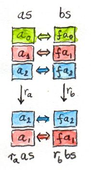
String concatenation is an interesting case, because we have a choice of defining right appenders and left appenders (or prependers, if you will). The composition tables of the two models are a mirror reverse of each other. You can easily convince yourself that appending “bar” after “foo” corresponds to prepending “foo” after prepending “bar”.

You might ask the question whether every categorical monoid — a one-object category — defines a unique set-with-binary-operator monoid. It turns out that we can always extract a set from a single-object category. This set is the set of morphisms — the adders in our example. In other words, we have the hom-set M(m, m) of the single object m in the category M. We can easily define a binary operator in this set: The monoidal product of two set-elements is the element corresponding to the composition of the corresponding morphisms. If you give me two elements of M(m, m) corresponding to f and g, their product will correspond to the composition g∘f. The composition always exists, because the source and the target for these morphisms are the same object. And it’s associative by the rules of category. The identity morphism is the neutral element of this product. So we can always recover a set monoid from a category monoid. For all intents and purposes they are one and the same.

Monoid hom-set seen as morphisms and as points in a set

Monoid hom-set seen as morphisms and as points in a set

There is just one little nit for mathematicians to pick: morphisms don’t have to form a set. In the world of categories there are things larger than sets. A category in which morphisms between any two objects form a set is called locally small. As promised, I will be mostly ignoring such subtleties, but I thought I should mention them for the record.

A lot of interesting phenomena in category theory have their root in the fact that elements of a hom-set can be seen both as morphisms, which follow the rules of composition, and as points in a set. Here, composition of morphisms in M translates into monoidal product in the set M(m, m).

Acknowledgments

I’d like to thank Andrew Sutton for rewriting my C++ monoid concept code according to his and Bjarne Stroustrup’s latest proposal.

Challenges

  1. Generate a free category from:
    1. A graph with one node and no edges
    2. A graph with one node and one (directed) edge (hint: this edge can be composed with itself)
    3. A graph with two nodes and a single arrow between them
    4. A graph with a single node and 26 arrows marked with the letters of the alphabet: a, b, c … z.
  2. What kind of order is this?
    1. A set of sets with the inclusion relation: A is included in B if every element of A is also an element of B.
    2. C++ types with the following subtyping relation: T1 is a subtype of T2 if a pointer to T1 can be passed to a function that expects a pointer to T2 without triggering a compilation error.
  3. Considering that Bool is a set of two values True and False, show that it forms two (set-theoretical) monoids with respect to, respectively, operator && (AND) and || (OR).
  4. Represent the Bool monoid with the AND operator as a category: List the morphisms and their rules of composition.
  5. Represent addition modulo 3 as a monoid category.

Next: A programming example of pure functions that do logging using Kleisli categories.


Ferrari museum in Maranello

Ferrari museum in Maranello

I was recently visiting the Ferrari museum in Maranello, Italy, where I saw this display of telemetry data from racing cars.

Telemetry data from a racing car. The contour of the racing track is shown in the upper left corner and various data channels are displayed below.

Telemetry data from a racing car. The racing track is displayed in the upper left corner and various data channels are displayed below.

The processing and the display of telemetry data is an interesting programming challenge. It has application in space exploration (as in, when you land a probe on a surface of a comet), medicine, and the military. The same techniques are used in financial systems where streams carry information about stock prices, commodity prices, and currency exchange rates.

It’s also a problem that lends itself particularly well to functional programming. If you are one of these shops working with telemetry, and you have to maintain legacy code written in imperative style, you might be interested in an alternative approach, especially if you are facing constant pressure to provide more sophisticated analysis tools and introduce concurrency to make the system faster and more responsive.

What all these applications have in common is that they deal with multiple channels generating streams of data. The data has to be either displayed in real time or stored for later analysis and processing. It’s pretty obvious to a functional programmer that channels are functors, and that they should be composed using combinators. In fact this observation can drive the whole architecture. The clincher is the issue of concurrency: retrofitting non-functional code to run in parallel is a lost battle — it’s almost easier to start from scratch. But treating channels as immutable entities makes concurrency almost an after-thought.

Everything is a Number

The most basic (and totally wrong) approach is to look at telemetry as streams of numbers. This is the assembly language of data processing. When everything is a number and you can apply your math any way you wish. The problem is that you are throwing away a lot of useful information. You want to use types as soon as possible to encode additional information and to prevent nonsensical operations like adding temperature to velocity.

In an engineering application, the least you can do is to keep track of units of measurement. You also want to distinguish between channels that produce floating-point numbers and ones that produce integers, or Booleans, or strings. This immediately tells you that a channel should be a polymorphic data structure. You should be able to stream any type of data, be it bytes, complex numbers, or vectors.

Everything is an Object

To an object-oriented mind it looks very much like a channel should be an object that is parameterized by the type of data it carries. And as an object it should have some methods. We need the get method to access the current value, and the next method to increment the position in the stream. As an imperative programmer you might also be tempted to provide a mutator, set. If you ever want your program to be concurrent, don’t even think about it!

If you’re a C++ programmer, you may overload some operators, and use * and ++ instead. That would make a channel look more like a forward iterator. But whatever you call it, a functional programmer will recognize it as a list, with the head and tail functionality.

Everything is a List

Let’s talk about lists, because there is a lot of misunderstanding around them. When people think of lists in imperative languages they think about storage. A list is probably the worst data type for storing data. Imperative programmers naturally assume that functional programmers, who use lists a lot, must be crazy. They are not! A Haskell list is almost never used for storing bulk data. A list is either an interface to data that is stored elsewhere, or a generator of data. Haskell is a lazy functional language, so what looks like a data structure is really a bunch of functions that provide data on demand.

That’s why I wouldn’t hesitate to implement channels as lists in Haskell. As an added bonus, lists can provide a pull interface to data that is being pushed. Reactive programs that process streams of data may be written as if all the data were already there — the event handler logic can be hidden inside the objects that generate the data. And this is just what’s needed for live telemetry data.

Obviously, functional programming is easier in Haskell than in C++, C#, or Java. But given how much legacy software there is, it could be a lost cause to ask management to (a) throw away existing code and start from scratch, (b) retrain the team to learn a new language, and (c) deal with completely new performance characteristics, e.g., lazy evaluation and garbage collection. So, realistically, the best we can do is to keep introducing functional methods into imperative languages, at least for the time being. It doesn’t mean that Haskell should’t play an important role in it. Over and over again I find myself prototyping solutions in Haskell before translating them into C++. The added effort pays back handsomely through faster prototyping, better code quality, and fewer bugs to chase. So I would highly recommend to every imperative programmer to spend, say, an hour a day learning and playing with Haskell. You’d be amazed how it helps in developing your programming skills.

Everything is a Functor

So, if you’re an object oriented programmer, you’ll probably implement a channel as something like this:

template <class T> Channel {
    virtual T get();
    virtual bool next();
};

and then get stuck. With this kind of interface, the rest of your program is bound to degenerate into a complex system of loops that extract data from streams and process them, possibly stuffing it back into other streams.

Instead, I propose to try the functional way. I will show you some prototype code in Haskell, but mostly explain how things work, so a non-Haskell programmer can gain some insight.

Here’s the definition of a polymorphic channel type, Chan:

data Chan a = Chan [a]

where a plays the role of a type variable, analogous to T in the C++ code above. The right hand side of the equal sign defines the constructor Chan that takes a list as an argument. Constructors are used both for constructing and for pattern matching. The notation [a] means a list of a.

The details don’t really matter, as long as you understand that the channel is implemented as a list. Also, I’m making things a little bit more explicit for didactic purposes. A Haskell programmer would implement the channel as a type alias, type, rather than a separate type.

Rule number one of dealing with lists is: try not to access their elements in a loop (or, using the functional equivalent of a loop — recursively). Operate on lists holistically. For instance, one of the most common operations on lists is to apply a function to every element. That means we want our Chan to be a functor.

A functor is a polymorphic data type that supports operating on its contents with a function. In the case of Chan that’s easy, since a list itself is a functor. I’ll be explicit here, again for didactic reasons. This is how you make Chan an instance of the Functor class by defining how to fmap a function f over it:

instance Functor Chan where
    fmap f (Chan xs) = Chan (map f xs)

Here, map is a library function that applies f to every element of the list. This is very much like applying C++ std::transform to a container, except that in Haskell everything is evaluated lazily, so you can apply fmap to an infinite list, or to a list that is not there yet because, for instance, it’s being generated in real time from incoming telemetry.

Everything is a Combinator

Let’s see how far we can get with this channel idea. The next step is to be able to combine multiple channels to generate streams of derived data. For instance, suppose that you have one channel from a pressure gauge, and another providing volume data, and you want to calculate instantaneous temperature using the ideal gas equation.

Let’s start with defining some types. We want separate types for quantities that are measured using different units. Once more, I’m being didactic here, because there are ready-made Haskell libraries that use so called phantom types to encode measurement units. Here I’ll do it naively:

data Pressure = Pascal Float
data Volume   = Meter3 Float
data Temp     = Kelvin Float

I’ll also define the ideal gas constant:

constR = 8.314472 -- J/(mol·K)

Here’s the function that calculates the temperature of ideal gas:

getT :: Float -> Pressure -> Volume -> Temp
getT n (Pascal p) (Meter3 v) = Kelvin (p * v / (n * constR))

The question is, how can we apply this function to the pressure and volume channels to get the temperature channel? We know how to apply a function to a single channel using fmap, but here we have to work with two channels. Fortunately, a channel is not just a functor — it’s an applicative functor. It defines the action of multi-argument functions on multiple channels. I’ll give you a Haskell implementation, but you should be able to do the same in C++ by overloading fmap or transform.

instance Applicative Chan where
    pure x = Chan (repeat x)
    (Chan fs) <*> (Chan xs) = Chan (zipWith ($) fs xs)

The Applicative class defines two functions. One is called pure, and it creates a constant channel from a value by repeatedly returning the same value. The other is a binary operator <*> that applies a channel of functions (yes, you can treat functions the same way you treat any other data) to a channel of values. The function zipWith applies, pairwise, functions to arguments using the function application operator ($).

Again, the details are not essential. The bottom line is that this allows us to apply our function getT to two channels (actually, three channels, since we also need to provide the amount of gas in moles — here I’m assuming 0.1 moles).

chT :: Chan Pressure -> Chan Volume -> Chan Temp
chT chP chV = getT <$> pure 0.1 <*> chP <*> chV

Such functions that combine channels into new channels are called combinators, and an applicative functor makes the creation of new combinators very easy.

The combinators are not limited to producing physical quantities. They may as well produce channels of alerts, channels of pixels for display, or channels of visual widgets. You can construct the whole architecture around channels. And since we’ve been only considering functional data structures, the resulting architecture can be easily subject to parallelization.

Moving Average

But don’t some computations require mutable state? For instance, don’t you need some kind of accumulators in order to calculate, let’s say, moving averages? Let’s see how this can be done functionally.

The idea is to keep a running sum of list elements within a fixed window of size n. When advancing through the list, we will add the new incoming element to the running sum and subtract the old outgoing element. The average is just this sum divided by n.

We can use the old trick of delaying the list by n positions. We’ll pad the beginning of the delayed list with n zeros. Here’s the Haskell code:

delay :: Num a => Int -> [a] -> [a]
delay n lst = replicate n 0 ++ lst

The first line is the (optional, but very useful) type signature. The second line defines the function delay that takes the delay counter n and the list. The function returns a list that is obtained by concatenating (operator ++) the zero-filled list (replicate n 0) in front of the original list. For instance, if you start with the list [1, 2, 3, 4] and delay it by 2, you’ll get [0, 0, 1, 2, 3, 4].

The next step is to create a stream of deltas — the differences between elements separated by n positions. We do it by zipping two lists: the original and the delayed one.

zip lst (delay n lst)

The function zip pairs elements from the first list with the elements from the second list.

Continuing with our example, the zipping will produce the pairs [(1, 0), (2, 0), (3, 1), (4, 2)]. Notice that the left number in each pair is the incoming element that is to be added to the running sum, while the right number is the outgoing one, to be subtracted from the running sum.

Now if we subtract the two numbers in each pair we’ll get exactly the delta that has to be added to the running sum at each step. We do the subtraction by mapping the operator (-) over the list. (To make the subtraction operator (-) operate on pairs we have to uncurry it. (If you don’t know what currying is, don’t worry.)

deltas :: Num a => Int -> [a] -> [a]
deltas n lst = map (uncurry (-)) (zip lst (delay n lst))

Continuing with the example, we will get [1, 2, 2, 2]. These are the amounts by which the running sum should change at every step. (Incidentally, for n equal to one, the deltas are proportional to the derivative of the sampled stream.)

Finally, we have to start accumulating the deltas. There is a library function scanl1 that can be used to produce a list of partial sums when called with the summation operator (+).

slidingSums :: Num a => Int -> [a] -> [a]
slidingSums n lst =  scanl1 (+) (deltas n lst)

At each step, scanl1 will add the delta to the previous running sum. The “1” in its name means that it will start with the first element of the list as the accumulator. The result, in our little example, is [1, 3, 5, 7]. What remains is to divide each sum by n and we’re done:

movingAverage :: Fractional a => Int -> [a] -> [a]
movingAverage n list = map (/ (fromIntegral n)) (slidingSums n list)

Since n is an integer, it has to be explicitly converted to a fractional number before being passed to the division operator. This is done using fromIntegral. The slightly cryptic notation (/ (fromIntegral n)) is called operator section. It just means “divide by n.”

As expected, the final result for the two-element running average of [1, 2, 3, 4] is [0.5, 1.5, 2.5, 3.5]. Notice that we haven’t used any mutable state to achieve this result, which makes this code automatically thread safe. Also, because the calculation is lazy, we can calculate the moving average of an infinite list as long as we only extract a finite number of data points. Here, we are printing the first 10 points of the 5-element moving average of the list of integers from 1 to infinity.

print (take 10 (movingAverage 5 [1..]))

The result is:

[0.2, 0.6, 1.2, 2.0, 3.0, 4.0, 5.0, 6.0, 7.0, 8.0]

Conclusion

The functional approach is applicable to designing software not only in the small but, more importantly, in the large. It captures the patterns of interaction between components and the ways they compose. The patterns I mentioned in this post, the functor and the applicative functor, are probably the most common, but functional programmers have at their disposal a large variety of patterns borrowed from various branches of mathematics. These patterns can be used by imperative programmers as well, resulting in cleaner and more maintainable software that is, by construction, multithread-ready.


Table of Contents

Part One

  1. Category: The Essence of Composition
  2. Types and Functions
  3. Categories Great and Small
  4. Kleisli Categories
  5. Products and Coproducts
  6. Simple Algebraic Data Types
  7. Functors
  8. Functoriality
  9. Function Types
  10. Natural Transformations

Part Two

  1. Declarative Programming
  2. Limits and Colimits
  3. Free Monoids
  4. Representable Functors
  5. The Yoneda Lemma
  6. Yoneda Embedding

Part Three

  1. It’s All About Morphisms
  2. Adjunctions
  3. Free/Forgetful Adjunctions
  4. Monads: Programmer’s Definition
  5. Monads and Effects
  6. Monads Categorically
  7. Comonads
  8. F-Algebras
  9. Algebras for Monads
  10. Ends and Coends
  11. Kan Extensions
  12. Enriched Categories
  13. Topoi
  14. Lawvere Theories
  15. Monads, Monoids, and Categories

There is a free pdf version of this book with nicer typesetting available for download. You may order a hard-cover version with color illustrations at Blurb. Or you may watch me teaching this material to a live audience.

Preface

For some time now I’ve been floating the idea of writing a book about category theory that would be targeted at programmers. Mind you, not computer scientists but programmers — engineers rather than scientists. I know this sounds crazy and I am properly scared. I can’t deny that there is a huge gap between science and engineering because I have worked on both sides of the divide. But I’ve always felt a very strong compulsion to explain things. I have tremendous admiration for Richard Feynman who was the master of simple explanations. I know I’m no Feynman, but I will try my best. I’m starting by publishing this preface — which is supposed to motivate the reader to learn category theory — in hopes of starting a discussion and soliciting feedback.

I will attempt, in the space of a few paragraphs, to convince you that this book is written for you, and whatever objections you might have to learning one of the most abstract branches of mathematics in your “copious spare time” are totally unfounded.

My optimism is based on several observations. First, category theory is a treasure trove of extremely useful programming ideas. Haskell programmers have been tapping this resource for a long time, and the ideas are slowly percolating into other languages, but this process is too slow. We need to speed it up.

Second, there are many different kinds of math, and they appeal to different audiences. You might be allergic to calculus or algebra, but it doesn’t mean you won’t enjoy category theory. I would go as far as to argue that category theory is the kind of math that is particularly well suited for the minds of programmers. That’s because category theory — rather than dealing with particulars — deals with structure. It deals with the kind of structure that makes programs composable.

Composition is at the very root of category theory — it’s part of the definition of the category itself. And I will argue strongly that composition is the essence of programming. We’ve been composing things forever, long before some great engineer came up with the idea of a subroutine. Some time ago the principles of structured programming revolutionized programming because they made blocks of code composable. Then came object oriented programming, which is all about composing objects. Functional programming is not only about composing functions and algebraic data structures — it makes concurrency composable — something that’s virtually impossible with other programming paradigms.

Third, I have a secret weapon, a butcher’s knife, with which I will butcher math to make it more palatable to programmers. When you’re a professional mathematician, you have to be very careful to get all your assumptions straight, qualify every statement properly, and construct all your proofs rigorously. This makes mathematical papers and books extremely hard to read for an outsider. I’m a physicist by training, and in physics we made amazing advances using informal reasoning. Mathematicians laughed at the Dirac delta function, which was made up on the spot by the great physicist P. A. M. Dirac to solve some differential equations. They stopped laughing when they discovered a completely new branch of calculus called distribution theory that formalized Dirac’s insights.

Of course when using hand-waving arguments you run the risk of saying something blatantly wrong, so I will try to make sure that there is solid mathematical theory behind informal arguments in this book. I do have a worn-out copy of Saunders Mac Lane’s Category Theory for the Working Mathematician on my nightstand.

Since this is category theory for programmers I will illustrate all major concepts using computer code. You are probably aware that functional languages are closer to math than the more popular imperative languages. They also offer more abstracting power. So a natural temptation would be to say: You must learn Haskell before the bounty of category theory becomes available to you. But that would imply that category theory has no application outside of functional programming and that’s simply not true. So I will provide a lot of C++ examples. Granted, you’ll have to overcome some ugly syntax, the patterns might not stand out from the background of verbosity, and you might be forced to do some copy and paste in lieu of higher abstraction, but that’s just the lot of a C++ programmer.

But you’re not off the hook as far as Haskell is concerned. You don’t have to become a Haskell programmer, but you need it as a language for sketching and documenting ideas to be implemented in C++. That’s exactly how I got started with Haskell. I found its terse syntax and powerful type system a great help in understanding and implementing C++ templates, data structures, and algorithms. But since I can’t expect the readers to already know Haskell, I will introduce it slowly and explain everything as I go.

If you’re an experienced programmer, you might be asking yourself: I’ve been coding for so long without worrying about category theory or functional methods, so what’s changed? Surely you can’t help but notice that there’s been a steady stream of new functional features invading imperative languages. Even Java, the bastion of object-oriented programming, let the lambdas in C++ has recently been evolving at a frantic pace — a new standard every few years — trying to catch up with the changing world. All this activity is in preparation for a disruptive change or, as we physicist call it, a phase transition. If you keep heating water, it will eventually start boiling. We are now in the position of a frog that must decide if it should continue swimming in increasingly hot water, or start looking for some alternatives.

IMG_1299

One of the forces that are driving the big change is the multicore revolution. The prevailing programming paradigm, object oriented programming, doesn’t buy you anything in the realm of concurrency and parallelism, and instead encourages dangerous and buggy design. Data hiding, the basic premise of object orientation, when combined with sharing and mutation, becomes a recipe for data races. The idea of combining a mutex with the data it protects is nice but, unfortunately, locks don’t compose, and lock hiding makes deadlocks more likely and harder to debug.

But even in the absence of concurrency, the growing complexity of software systems is testing the limits of scalability of the imperative paradigm. To put it simply, side effects are getting out of hand. Granted, functions that have side effects are often convenient and easy to write. Their effects can in principle be encoded in their names and in the comments. A function called SetPassword or WriteFile is obviously mutating some state and generating side effects, and we are used to dealing with that. It’s only when we start composing functions that have side effects on top of other functions that have side effects, and so on, that things start getting hairy. It’s not that side effects are inherently bad — it’s the fact that they are hidden from view that makes them impossible to manage at larger scales. Side effects don’t scale, and imperative programming is all about side effects.

Changes in hardware and the growing complexity of software are forcing us to rethink the foundations of programming. Just like the builders of Europe’s great gothic cathedrals we’ve been honing our craft to the limits of material and structure. There is an unfinished gothic cathedral in Beauvais, France, that stands witness to this deeply human struggle with limitations. It was intended to beat all previous records of height and lightness, but it suffered a series of collapses. Ad hoc measures like iron rods and wooden supports keep it from disintegrating, but obviously a lot of things went wrong. From a modern perspective, it’s a miracle that so many gothic structures had been successfully completed without the help of modern material science, computer modelling, finite element analysis, and general math and physics. I hope future generations will be as admiring of the programming skills we’ve been displaying in building complex operating systems, web servers, and the internet infrastructure. And, frankly, they should, because we’ve done all this based on very flimsy theoretical foundations. We have to fix those foundations if we want to move forward.

Ad hoc measures preventing the Beauvais cathedral from collapsing

Ad hoc measures preventing the Beauvais cathedral from collapsing

Next: Category: The Essence of Composition.


Data races lead to undefined behavior; but how bad can they really be? In my previous post I talked about benign data races and I gave several examples taken from the Windows kernel. Those examples worked because the kernel was compiled with a specific compiler for a specific processor. But in general, if you want your code to be portable, you can’t have data races, period.

You just cannot reason about something that is specifically defined to be “undefined.” So, obviously, you cannot prove the correctness of a program that has data races. However, very few people engage in proofs of correctness. In most cases the argument goes, “I can’t see how this can fail, therefore it must be correct” (maybe not in so many words). I call this “proof by lack of imagination.” If you want to become a concurrency expert, you have to constantly stretch your imagination. So let’s do a few stretches.

One of the readers of my previous post, Duarte Nunes, posted a very interesting example of a benign data race. Here’s the code:

int owner = 0;
int count = 0;
std::mutex mtx;

bool TryEnter() {
    if (owner == std::this_thread::get_id()) {
        count += 1;
        return true;
    }

    if (mtx.try_lock()) {
        owner = std::this_thread::get_id();
        return true;
    }
    return false;
}

void Exit() {
    if (count != 0) {
        count -= 1;
        return;
    }
    owner = 0;
    mtx.unlock();
}

I highlighted in blue the parts that are executed under the lock (in a correct program, Exit will always be called after the lock has been acquired). Notice that the variable count is always accessed under the lock, so no data races there. However, the variable owner may be read outside of the lock– I highlighted that part of code in red. That’s the data race we are talking about.

Try to analyze this code and imagine what could go wrong. Notice that the compiler or the processor can’t be too malicious. The code still has to work correctly if the data race is removed, for instance if the racy read is put under the lock.

Here’s an attempt at the “proof” of correctness. First, Duarte observed that “The valid values for the owner variable are zero and the id of any thread in the process.” That sort of makes sense, doesn’t it? Now, the only way the racy read can have any effect is if the value of owner is equal to the current thread’s ID. But that’s exactly the value that could have been written only by the current thread– and under the lock.

There are two possibilities when reading owner: either we are still under that lock, in which case the read is not at all racy; or we have already released the lock. But the release of the lock happens only after the current thread zeroes owner.

Notice that this is a single-thread analysis and, within a single thread, events must be ordered (no need to discuss memory fences or acquire/release semantics at this point). A read following a write in the same thread cannot see the value that was there before the write. That would break regular single-threaded programs. Of course, other threads may have overwritten this zero with their own thread IDs, but never with the current thread ID. Or so the story goes…

Brace yourself: Here’s an example how a compiler or the processor may “optimize” the program:

void Exit() {
    if (count != 0) {
        count -= 1;
        return;
    }
    owner = 42;
    owner = 0;
    mtx.unlock();
}

You might argue that this is insane and no compiler in its right mind would do a thing like this; but the truth is: It’s a legal program transformation. The effect of this modification is definitely not observable in the current thread. Neither is it observable by other threads in the absence of data races. Now, the unfortunate thread whose ID just happens to be 42 might observe this value and take the wrong turn. But it can only observe it through a racy read. For instance, it would never see this value if it read owner under the lock. Moreover, it would never see it if the variable owner were defined as ‘atomic’:

std::atomic<int> owner = 0

Stores and loads of atomic variables are, by default, sequentially consistent. Unfortunately sequential consistency, even on an x86, requires memory fences, which can be quite costly. It would definitely be an overkill in our example. So here’s the trick: Tell the compiler to forgo sequential consistency on a per read/write basis. For instance, here’s how you read an atomic variable without imposing any ordering constraints:

owner.load(memory_order_relaxed)

Such ‘relaxed’ operations will not introduce any memory fences– at least not on any processor I know about.

Here’s the version of the code that is exactly equivalent to the original, except that it’s correct and portable:

std::atomic<int> owner = 0;
int count = 0;
std::mutex mtx;

bool TryEnter() {
    if (owner.load(memory_order_relaxed) == std::this_thread::get_id()) {
        count += 1;
        return true;
    }

    if (mtx.try_lock()) {
        owner.store(std::this_thread::get_id(), memory_order_relaxed);
        return true;
    }
    return false;
}

void Exit() {
    if (count != 0) {
        count -= 1;
        return;
    }
    owner.store(0, memory_order_relaxed);
    mtx.unlock();
}

So what has changed? Can’t the compiler still do the same dirty trick, and momentarily store 42 in the owner variable? No, it can’t! Since the variable is declared ‘atomic,’ the compiler can no longer assume that the write can’t be observed by other threads.

The new version has no data races: The Standard specifically states that ‘atomic’ variables don’t contribute to data races, even in their most relaxed form.

C++ Standard, (1.10.5):
[…] “Relaxed” atomic operations are not synchronization operations even though, like synchronization operations, they cannot contribute to data races.

With those changes, I believe that our “proof” of correctness may actually be turned into a more rigorous proof using the axioms of the C++ memory model (although I’m not prepared to present one). We can have our cake (correct, portable code) and eat it too (no loss of performance). And, by the way, the same trick may be used in the case of lossy counters from my previous post.

Warning: I do not recommend this style of coding, or the use of weak atomics, to anybody who is not implementing operating system kernels or concurrency libraries.

Acknowledgments

I’d like to thank Luis Ceze, Hans Boehm, and Anthony Williams for useful remarks and for verifying my assumptions about the C++ memory model.

Bibliography

  1. C++ Draft Standard

We have this friendly competition going on between Eric Niebler and myself. He writes some clever C++ template code, and I feel the compulsion to explain it to him in functional terms. Then I write a blog about Haskell or category theory and Eric feels a compulsion to translate it into C++.

Eric is now working on his proposal to rewrite the C++ STL in terms of ranges and I keep reinterpreting his work in terms familiar to functional programmers. Eric’s range comprehensions are a result of some of this back and forth.

Lazy ranges are such an excellent example of functional programming that it would be foolish for me to pass this opportunity to dissect them. To any functional programmer worth their salt they just scream “monad!” A monad is a higher order pattern that can be built step by step, so that’s what I’m going to do. I’ll start with the functor pattern, then add some functionality that will make it a pointed functor, then add some more to make it an applicative functor, and finally add some more to make it a monad. This gradual buildup of functionality is reminiscent of building a class hierarchy, and indeed it can be modelled as such in Haskell (although Haskell type classes are slightly different than C++ classes). This hierarchy would look something like this:

  • A monad is-an applicative functor
  • An applicative functor is-a pointed functor
  • A pointed functor is-a functor

So let’s start with a functor.

Functor

I have a pet peeve about the use of the word “functor” in C++. People keep calling function objects functors. It’s like calling Luciano Pavarotti an “operator,” because he sings operas. The word functor has a very precise meaning in mathematics — moreover, it’s the branch of mathematics that’s extremely relevant to programming. So hijacking this term to mean a function-like object causes unnecessary confusion.

A functor in functional programming is a generic template, which allows the “lifting” of functions. Let me explain what it means. A generic template takes an arbitrary type as a template argument. So a range (whether lazy or eager) is a generic template because it can be instantiated for any type. You can have a range of integers, a range of vectors, a range of ranges, and so on. (We’ll come back to ranges of ranges later when we talk about monads.)

The “lifting” of functions means this: Give me any function from some type T to some other type U and I can apply this function to a range of T and produce a range of U. You may recognize this kind of lifting in the STL algorithm std::transform, which can be used to apply a function to a container. STL containers are indeed functors. Unfortunately, their functorial nature is buried under the noise of iterators. In Eric’s range library, the lifting is done much more cleanly using view::transform. Have a look at this example:

 int total = accumulate(view::iota(1) |
                        view::transform([](int x){return x*x;}) |
                        view::take(10), 0);

Here, view::transform takes an anonymous function that squares its argument, and lifts this function to the level of ranges. The range created by view::iota(1) is piped into it from the left, and the resulting rage of squares emerges from it on the right. The (infinite) range is then truncated by take‘ing the first 10 elements.

The function view::iota(1) is a factory that produces an infinite range of consecutive integers starting from 1. (We’ll come back to range factories later.)

In this form, view::transform plays the role of a higher-order function: one that takes a function and returns a function. It almost reaches the level of terseness and elegance of Haskell, where this example would look something like this:

total = sum $ take 10 $ fmap (\x->x*x) [1..]

(Traditionally, the flow of data in Haskell is from right to left.) The (higher-order) function fmap can be thought of as a “method” of the class Functor that does the lifting in Haskell. In C++ there is no overall functor abstraction, so each functor names its lifting function differently — for ranges, it’s view::transform.

The intuition behind a functor is that it generates a family of objects that somehow encapsulate values of arbitrary types. This encapsulation can be very concrete or very abstract. For instance, a container simply contains values of a given type. A range provides access to values that may be stored in some other container. A lazy range generates values on demand. A future, which is also a functor (or will be, in C++17), describes a value that might not be currently available because it’s being evaluated in a separate thread.

All these objects have one thing in common: they provide means to manipulate the encapsulated values with functions. That’s the only requirement for a functor. It’s not required that a functor provide access to encapsulated values (which may not even exist), although most do. In fact there is a functor (really, a monad), in Haskell, that provides no way of accessing its values other than outputting them to external devices.

Pointed Functor

A pointed functor is a functor with one additional ability: it lets you lift individual values. Give me a value of any type and I will encapsulate it. In Haskell, the encapsulating function is called pure although, as we will see later, in the context of a monad it’s called return.

All containers are pointed, because you can always create a singleton container — one that contains only one value. Ranges are more interesting. You can obviously create a range from a singleton container. But you can also create a lazy range from a value using a (generic) function called view::single, which doesn’t have a backing container behind it.

There is, however, an alternative way of lifting a value to a range, and that is by repeating it indefinitely. The function that creates such infinite (lazy) ranges is called view::repeat. For instance, view::repeat(1) creates an infinite series of ones. You might be wondering what use could there be of such a repetitive range. Not much, unless you combine it with other ranges. In general, pointed functors are not very interesting other than as stepping stones towards applicative functors and monads. So let’s move on.

Applicative Functor

An applicative functor is a pointed functor with one additional ability: it lets you lift multi-argument functions. We already know how to lift a single-argument function using fmap (or transform, or whatever it’s called for a particular functor).

With multi-argument functions acting on ranges we have two different options corresponding to the two choices for pure I mentioned before: view::single and view::repeat.

The idea, taken from functional languages, is to consider what happens when you provide the first argument to a function of multiple arguments (it’s called partial application). You don’t get back a value. Instead you get something that expects one or more remaining arguments. A thing that expects arguments is called a function (or a function object), so you get back a function of one fewer arguments. In C++ you can’t just call a function with fewer arguments than expected, or you get a compilation error, but there is a (higher-order) function in the Standard Library called std::bind that implements partial application.

This kind of transformation from a function of multiple arguments to a function of one argument that returns a function is called currying.

Let’s consider a simple example. We want to apply std::make_pair to two ranges: view::ints(10, 11) and view::ints(1, 3). To this end, let’s replace std::make_pair with the corresponding curried function of one argument returning a function of one argument:

[](int i) { return [i](int j) { return std::make_pair(i, j); };}

First, we want to apply this function to the first range. We know how to apply a function to a range: we use view::transform.

auto partial_app = view::ints(10, 11) 
                 | view::transform([](int i) { 
                      return [i](int j) { return std::make_pair(i, j); }
                   });

What’s the result of this application? Can you guess? Our curried function will be applied to each integer in the range, returning a function that pairs that integer with its argument. So we end up with a range of functions of the form:

[i](int j) { return std::make_pair(i, j); }

So far so good — we have just used the functorial property of the range. But now we have to decide how to apply a range of functions to the second range of values. And that’s the essence of the definition of an applicative functor. In Haskell the operation of applying encapsulated functions to encapsulated arguments is denoted by an infix operator <*>.

With ranges, there are two basic strategies:

  1. We can enumerate all possible combinations — in other words create the cartesian product of the range of functions with the range of values — or
  2. Match corresponding functions to corresponding values — in other words, “zip” the two ranges.

The former, when applied to view::ints(1, 3), will yield:

{(10,1),(10,2),(10,3),(11,1),(11,2),(11,3)}

and the latter will yield:

{(10, 1),(11, 2)}

(when the ranges are not equal length, you stop zipping when the shorter one is exhausted).

To see that those two choices correspond to the two choices for pure, we have to look at some consistency conditions. One of them is that if you encapsulate a single-argument function in a range using pure and then apply it to a range of arguments, you should get the same result as if you simply fmapped this function directly over the range of arguments. For the record, I’ll write it here in Haskell:

pure f <*> xs == fmap f xs

This is sort of an obvious requirement: You have two different ways of applying a single-argument function to a range, they better give the same result.

Let’s try it with the view::single version of pure. When acting on a function, it will create a one-element range containing this function. The “all possible combinations” application will just apply this function to all elements of the argument range, which is exactly what view::transform would do.

Conversely, if we apply view::repeat to the function, we’ll get an infinite range that repeats this function at every position. We have to zip this range with the range of arguments in order to get the same result as view::transform. So this implementation of pure works with the zippy applicative. Notice that if the argument range is finite the result will also be finite. But this kind of application will also work with infinite ranges thanks to laziness.

So there are two legitimate implementations of the applicative functor for ranges. One uses view::single to lift values and uses the all possible combinations strategy to apply a range of functions to a range of arguments. The other uses view::repeat to lift values and the zipping application for ranges of functions and arguments. They are both acceptable and have their uses.

Now let’s go back to our original problem of applying a function of multiple arguments to a bunch of ranges. Since we are not doing it in Haskell, currying is not really a practical option.

As it turns out, the second version of applicative has been implemented by Eric as a (higher-order) function view::zip_with. This function takes a multi-argument callable object as its first argument, followed by a variadic list of ranges.

There is no corresponding implementation for the combinatorial applicative. I think the most natural interface would be an overload of view::transform (or maybe view::fmap) with the same signature as zip_with. Our example would then look like this:

view::transform(std::make_pair, view::ints(10, 11), view::ints(1, 3));

The need for this kind of interface is not as acute because, as we’ll learn next, the combinatorial applicative is supplanted by a more general monadic interface.

Monad

Monads are applicative functors with one additional functionality. There are two equivalent ways of describing this functionality. But let me first explain why this functionality is needed.

The range library comes with a bunch of range factories, such as view::iota, view::ints, or view::repeat. It’s also very likely that users of the library will want to create their own range factories. The problem is: How do you compose existing range factories to obtain new range factories?

Let me give you an example that generated a blog post exchange between me and Eric. The challenge was to generate a list of Pythagorean triples. The idea is to take a cross product of three infinite ranges of integers and select those triples that satisfy the equation x2 + y2 = z2. The cross product of ranges is reminiscent of the “all possible combinations” applicative, and indeed that’s the applicative that can be extended to a monad (the zippy one can’t).

To make this algorithm feasible, we have to organize these ranges so we can (lazily) traverse them. Let’s start with a factory that produces all integers from 1 to infinity. That’s the view::ints(1) factory. Then, for each z produced by that factory, let’s create another factory view::ints(1, z). This range will provide our xs — and it makes no sense to try xs that are bigger than zs. These values, in turn, will be used in the creation of the third factory, view::ints(x, z) that will generate our ys. At the end we’ll filter out the triples that don’t satisfy the Pythagorean equation.

Notice how we are feeding the output of one range factory into another range factory. Do you see the problem? We can’t just iterate over an infinite range. We need a way to glue the output side of one range factory to the input side of another range factory without unpacking the range. And that’s what monads are for.

Remember also that there are functors that provide no way of extracting values, or for which extraction is expensive or blocking (as is the case with futures). Being able to compose those kinds of functor factories is often essential, and again, the monad is the answer.

Now let’s pinpoint the type of functionality that would allow us to glue range factories end-to-end. Since ranges are functorial, we can use view::transform to apply a factory to a range. After all a factory is just a function. The only problem is that the result of such application is a range of ranges. So, really, all that’s needed is a lazy way of flattening nested ranges. And that’s exactly what Eric’s view::flatten does.

With this new flattening power at our disposal, here’s a possible beginning of the solution to the Pythagorean triple problem:

view::ints(1) | view::transform([](int z) { 
                view::ints(1, z) | ... } | view::flatten

However, this combination of view::transform and view::flatten is so useful that it deserves its own function. In Haskell, this function is called “bind” and is written as an infix operator >>=. (And, while we’re at it, flatten is called join.)

And guess what the combination of view::transform and view::flatten is called in the range library. This discovery struck me as I was looking at one of Eric’s examples. It’s called view::for_each. Here’s the solution to the Pythagorean triple problem using view::for_each to bind range factories:

auto triples =
  for_each(ints(1), [](int z) {
    return for_each(ints(1, z), [=](int x) {
      return for_each(ints(x, z), [=](int y) {
        return yield_if(x*x + y*y == z*z, std::make_tuple(x, y, z));
      });
    });
  });

And here’s the same code in Haskell:

triples = 
  (>>=) [1..] $ \z -> 
     (>>=) [1..z] $ \x -> 
        (>>=) [x..z] $ \y -> 
           guard (x^2 + y^2 == z^2) >> return (x, y, z)

I have purposefully re-formatted Haskell code to match C++ (A more realistic rendition of it is in my post Getting Lazy with C++). Bind operators >>= are normally used in infix position but here I wanted to match them against for_each. Haskell’s return is the same as view::single, which Eric renamed to yield inside for_each. In this particular case, yield is conditional, which in Haskell is expressed using guard. The syntax for lambdas is also different, but otherwise the code matches almost perfectly.

This is an amazing and somewhat unexpected convergence. In our tweeter exchange, Eric sheepishly called his for_each code imperative. We are used to thinking of for_each as synonymous with looping, which is such an iconic imperative construct. But here, for_each is the monadic bind — the epitome of functional programming. This puppy is purely functional. It’s an expression that returns a value (a range) and has no side effects.

But what about those loops that do have side effects and don’t return a value? In Haskell, side effects are always encapsulated using monads. The equivalent of a for_each loop with side effects would return a monadic object. What we consider side effects would be encapsulated in that object. It’s not the loop that performs side effects, its that object. It’s an executable object. In the simplest case, this object contains a function that may be called with the state that is to be modified. For side effects that involve the external world, there is a special monad called the IO monad. You can produce IO objects, you can compose them using monadic bind, but you can’t execute them. Instead you return one such object that combines all the IO of your program from main and let the runtime execute it. (At least that’s the theory.)

Is this in any way relevant to an imperative programmer? After all, in C++ you can perform side effects anywhere in your code. The problem is that there are some parts of your code where side effects can kill you. In concurrent programs uncontrolled side effects lead to data races. In Software Transactional Memory (STM, which at some point may become part of C++) side effects may be re-run multiple times when a transaction is retried. There is an urgent need to control side effects and to separate pure functions from their impure brethren. Encapsulating side effects inside monads could be the ticket to extend the usefulness of pure functions inside an imperative language like C++.

To summarize: A monad is an applicative functor with an additional ability, which can be expressed either as a way of flattening a doubly encapsulated object, or as a way of applying a functor factory to an encapsulated object.

In the range library, the first method is implemented through view::flatten, and the second through view::for_each. Being an applicative functor means that a range can be manipulated using view::transform and that any value may be encapsulated using view::single or, inside for_each, using yield.

The ability to apply a range of functions to a range of arguments that is characteristic of an applicative functor falls out of the monadic functionality. For instance, the example from the previous section can be rewritten as:

for_each(ints(10, 11), [](int i) {
  return for_each(ints(1, 3), [i](int j) {
    return yield(std::make_pair(i, j));
  });
});

The Mess We’re In

I don’t think the ideas I presented here are particularly difficult. What might be confusing though is the many names that are used to describe the same thing. There is a tendency in imperative (and some functional) languages to come up with cute names for identical patterns specialized to different applications. It is also believed that programmers would be scared by terms taken from mathematics. Personally, I think that’s silly. A monad by any other name would smell as sweet, but we wouldn’t be able to communicate about them as easily. Here’s a sampling of various names used in relation to concepts I talked about:

  1. Functor: fmap, transform, Select (LINQ)
  2. Pointed functor: pure, return, single, repeat, make_ready_future, yield, await
  3. Applicative functor: <*>, zip_with
  4. Monad: >>=, bind, mbind, for_each, next, then, SelectMany (LINQ)

Part of the problem is the lack of expressive power in C++ to unite such diverse phenomena as ranges and futures. Unfortunately, the absence of unifying ideas adds to the already overwhelming complexity of the language and its libraries. The functional paradigm could be a force capable of building connections between seemingly distant application areas.

Acknowledments

I’m grateful to Eric Niebler for reviewing the draft of this blog and correcting several mistakes. The remaining mistakes are all mine.


Can a data race not be a bug? In the strictest sense I would say it’s always a bug. A correct program written in a high-level language should run the same way on every processor present, past, and future. But there is no proscription, or even a convention, about what a processor should (or shouldn’t) do when it encounters a race. This is usually described in higher-level language specs by the ominous phrase: “undefined behavior.” A data race could legitimately reprogram your BIOS, wipe out your disk, and stop the processor’s fan causing a multi-core meltdown.

Data race: Multiple threads accessing the same memory location without intervening synchronization, with at least one thread performing a write.

However, if your program is only designed to run on a particular family of processors, say the x86, you might allow certain types of data races for the sake of performance. And as your program matures, i.e., goes through many cycles of testing and debugging, the proportion of buggy races to benign races keeps decreasing. This becomes a real problem if you are using a data-race detection tool that cannot distinguish between the two. You get swamped by false positives.

Microsoft Research encountered and dealt with this problem when running their race detector called DataCollider on the Windows kernel (see Bibliography). Their program found 25 actual bugs, and almost an order of magnitude more benign data races. I’ll summarize their methodology and discuss their findings about benign data races.

Data Races in the Windows Kernel

The idea of the program is very simple. Put a hardware breakpoint on a shared memory access and wait for one of the threads to stumble upon it. This is a code breakpoint, which is triggered when the particular code location is executed. The x86 also supports another kind of a breakpoint, which is called a data breakpoint, triggered when the program accesses a specific memory location. So when a thread hits the code breakpoint, DataCollider installs a data breakpoint at the location the thread was just accessing. It then stalls the current thread and lets all other threads run. If any one of them hits the data breakpoint, it’s a race (as long as one of the accesses is a write). Consider this: If there was any synchronization (say, a lock acquisition was attempted) between the two accesses, the second thread would have been blocked from accessing that location. Since it wasn’t, it’s a classic data race.

Notice that this method might not catch all data races, but it doesn’t produce false positives. Except, of course, when the race is considered benign.

There are other interesting details of the algorithm. One is the choice of code locations for installing breakpoints. DataCollider first analyzes the program’s assembly code to create a pool of memory accesses. It discards all thread-local accesses and explicitly synchronized instructions (for instance, the ones with the LOCK prefix). It then randomly picks locations for breakpoints from this pool. Notice that rarely executed paths are as likely to be sampled as the frequently executed ones. This is important because data races, like fugitive criminals, often hide in less frequented places.

Pruning Benign Races

90% of data races caught by DataCollider in the Windows kernel were benign. For several reasons it’s hard to say how general this result is. First, the kernel had already been tested and debugged for some time, so many low-hanging concurrency bugs have been picked. Second, operating system kernels are highly optimized for a particular processor and might use all kinds of tricks to improve performance. Finally, kernels often use unusual synchronization strategies. Still, it’s interesting to see what shape benign data races take.

It turns out that half of all false positives came from lossy counters. There are many places where statistics are gathered: counting certain kinds of events, either for reporting or for performance enhancements. In those situations losing a few increments is of no relevance. However not all counters are lossy and, for instance, a data race in reference counting is a serious bug. DataCollider uses simple heuristic to detect lossy counters–they are the ones that are always incremented. A reference counter, on the other hand, is as often incremented as decremented.

Another benign race happens when one thread reads a particular bit in a bitfield while another thread updates another bit. A bit update is a read-modify-write (RMW) sequence: The thread reads the previous value of the bitfield, modifies one bit, and writes the whole bitfield back. Other bits are overwritten in the process too, but their new values are the same as the old values. A read from another thread of any of the the non-changed bits does not interfere with the write, at least not on the x86. Of course if yet another thread modified one of those bits, it would be a real bug, and it would be caught separately. The pruning of this type of race requires analysis of surrounding code (looking for the masking of other bits).

Windows kernel also has some special variables that are racy by design–current time is one such example. DataCollider has these locations hard-coded and automatically prunes them away.

There are benign races that are hard to prune automatically, and those are left for manual pruning (in fact, DataCollider reports all races, it just de-emphasizes the ones it considers benign). One of them is the double-checked locking pattern (DCLP), where a thread makes a non-synchronized read to be later re-confirmed under the lock. This pattern happens to work on the x86, although it definitely isn’t portable.

Finally, there is the interesting case of idempotent writes— two racing writes that happen to write the same value to the same location. Even though such scenarios are easy to prune, the implementers of DataCollider decided not to prune them because more often than not they led to the uncovering of concurrency bugs. Below is a table that summarizes various cases.

Benign race Differentiate from Pruned?
Lossy counter Reference counting Yes
Read and write of different bits Read and write of the whole word Yes
Deliberately racy variables Yes
DCLP No
Idempotent writes No

Conclusion

In the ideal world there would be no data races. But a concurrency bug detector must take into account the existence of benign data races. In the early stages of product testing the majority of detected races are real bugs. It’s only when chasing the most elusive of concurrency bugs that it becomes important to weed out benign races. But it’s the elusive ones that bite the hardest.

Bibliography

  1. John Erickson, Madanlal Musuvathi, Sebastian Burckhardt, Kirk Olynyk, Effective Data-Race Detection for the Kernel

I’m not fond of arguments based on lack of imagination. “There’s no way this code may fail!” might be a sign of great confidence or the result of ignorance. The inability to come up with a counterexample doesn’t prove a theorem. And yet there is one area of programming where such arguments work, and are quite useful. These are parametricity arguments: free theorems about polymorphic functions. Fortunately, there is solid theory behind parametricity. Free theorems are not based on ignorance. So I decided to read the relevant papers (see bibliography at the end of this post) and write a blog about it. How hard could it be? A few months and several failed attempts later I realized how naive I was. But I think I finally understand the basics enough to explain them in relatively simple terms.

Motivation

Here’s a classic example — a function that takes a list of arbitrary type a and returns a list of the same type:

r :: [a] -> [a]

What can this function do? Since it has to work with any type of list element, it can’t do anything type-specific. It can’t modify the elements or invent new ones. So all it can do is rearrange them, duplicate, or remove. Can you think of anything else?

The questions it a little tricky because it all depends on the kind of polymorphism your language supports. In Haskell, where we have parametric polymorphism, the above statement is for the most part true (modulo termination worries). In C++, which supports ad-hoc polymorphism, a generic function like:

template<class T> 
list<T> r(list<T>);

can do all kinds of weird things.

Parametric polymorphism means that a function will act on all types uniformly, so the above declaration of r indeed drastically narrows down the possibilities.

For instance, consider what happens when you map any function of the type:

f :: a -> b

over a list of a. You can either apply map before or after acting on it with r. It shouldn’t matter whether you first modify the elements of the list and then rearrange them, or first rearrange and then modify them. The result should be the same:

r (map f as) = map f (r as)

But is it true just because we can’t imagine how it may fail, or can we make a formal argument to prove it?

Let’s Argue (Denotational) Semantics

One way to understand polymorphism is to have a good model for types. At first approximation types can be modeled as sets of values (strictly speaking, as shown by Reynolds, the set-theoretical model fails in the case of polymorphic lambda calculus, but there are ways around it).

The type Bool is a two-element set of True and False, Integer is a set of integers, and so on. Composite types can also be defined set-theoretically. For instance, a pair type is a cartesian product of two sets. A list of a is a set of lists with elements from the set a. A function type a->b is a set of functions between two sets.

For parametric polymorphism you need to first be able to define functions on types: functions that take a type and produce a new type. In other words, you should be able to define a family of types that is parametrized by another type. In Haskell, we call such things type constructors.

For instance, given some type a, produce a type of pairs: (a, a). This can be formally written (not in Haskell) as:

Λa . (a, a)

Notice the capital lambda for defining functions on types (sets), as opposed to the lowercase lambda used for functions on values (set elements).

To turn a family of types into a family of values — a polymorphic value — you put the universal quantifier forall in front of it. Don’t read too much into the quantifier aspect of it — it makes sense in the Curry-Howard isomorphism, but here it’s just a piece of syntax. It means that you use the type constructor to pick a type, and then you pick a specific value of that type.

You may recall the Axiom of Choice (AoC) from set theory. This axiom says that if you have a set of sets then there always exists a set of samples created by picking one element from each set. It’s like going to a chocolate store and ordering one of each. It’s a controversial axiom, and mathematicians are very careful in either using or avoiding it. The controversy is that, for infinite sets of sets, there may be no constructive way of picking elements. And in computer science we are not so much interested in proofs of existence, as in actual algorithms that produce tangible results.

Here’s an example:

forall a . (a, a)

This is a valid type signature, but you’d be hard pressed to implement it. You’d have to provide a pair of concrete values for every possible type. You can’t do it uniformly across all types. (Especially that some types are uninhabited, as Gershom Bazerman kindly pointed out to me.)

Interestingly enough, you can sometimes define polymorphic values if you constrain polymorphism to certain typeclasses. For instance, when you define a numeric constant in Haskell:

x = 1

its type is polymorphic:

x :: forall a. Num a => a

(using the language extension ExplicitForAll). Here x represents a whole family of values, including:

1.0 :: Float
1 :: Int
1 :: Integer

with potentially different representations.

But there are some types of values that can be specified wholesale. These are function values. Functions are first class values in Haskell (although you can’t compare them for equality). And with one formula you can define a whole family of functions. The following signature, for instance, is perfectly implementable:

forall a . a -> a

Let’s analyze it. It consists of a type function, or a type constructor:

Λa . a -> a

which, for any type a, returns a function type a->a. When universally quantified with forall, it becomes a family of concrete functions, one per each type. This is possible because all these functions can be defined with one closed term (see Appendix 2). Here’s this term:

\x -> x

In this case we actually have a constructive way of picking one element — a function — for each type a. For instance, if a is a String, we pick a function that takes any String and returns the same string. It’s a particular String->String function, one of many possible String->String functions. And it’s different from the Int->Int function that takes an Int and returns the same Int. But all these identity functions are encoded using the same lambda expression. It’s that generic formula that allows us to chose a representative function from each set of functions a->a: one from the set String->String, one from the set Int->Int, etc.

In Haskell, we usually omit the forall quantifier when there’s no danger of confusion. Any signature that contains a type variable is automatically universally quantified over it. (You’ll have to use explicit forall, however, with higher-order polymorphism, where a polymorphic function can be passed as an argument to another function.)

So what’s the set-theoretic model for polymorphism? You simply replace types with sets. A function on types becomes a function on sets. Notice that this is not the same as a function between sets. The latter assigns elements of one set to elements of another. The former assigns sets to sets — you could call it a set constructor. As in: Take any set a and return a cartesian product of this set with itself.

Or take any set a and return the set of functions from this set to itself. We have just seen that for this one we can easily build a polymorphic function — one which for every type a produces an actual function whose type is (a->a). Now, with ad-hoc polymorphism it’s okay to code the String function separately from the Int function; but in parametric polymorphism, you’ll have to use the same code for all types.

This uniformity — one formula for all types — dramatically restricts the set of polymorphic functions, and is the source of free theorems.

Any language that provides some kind of pattern-matching on types (e.g., template specialization in C++) automatically introduces ad-hoc polymorphism. Ad-hoc polymorphism is also possible in Haskell through the use of type classes and type families.

Preservation of Relations

Let’s go to our original example and rewrite it using the explicit universal quantifier:

r :: forall a. [a] -> [a]

It defines a family of functions parametrized by the type a. When used in Haskell code, a particular member of this family will be picked automatically by the type inference system, depending on the context. In what follows, I’ll use explicit subscripting for the same purpose. The free theorem I mentioned before can be rewritten as:

rb (map f as) = map f (ra as)

with the function:

f :: a -> b

serving as a bridge between the types a and b. Specifically, f relates values of type a to values of type b. This relation happens to be functional, which means that there is only one value of type b corresponding to any given value of type a.

But the correspondence between elements of two lists may, in principle, be more general. What’s more general than a function? A relation. A relation between two sets a and b is defined as a set of pairs — a subset of the cartesian product of a and b. A function is a special case of a relation, one that can be represented as a set of pairs of the form (x, f x), or in relational notation x <=> f x. This relation is often called the graph of the function, since it can be interpreted as coordinates of points on a 2-d plane that form the plot the function.

The key insight of Reynolds was that you can abstract the shape of a data structure by defining relations between values. For instance, how do we know that two pairs have the same shape — even if one is a pair of integers, say (1, 7), and the other a pair of colors, say (Red, Blue)? Because we can relate 1 to Red and 7 to Blue. This relation may be called: “occupying the same position”.

Notice that the relation doesn’t have to be functional. The pair (2, 2) can be related to the pair (Black, White) using the non-functional relation:

(2 <=> Black),
(2 <=> White)

This is not a function because 2 is not mapped to a single value.

Conversely, given any relation between integers and colors, you can easily test which integer pairs are related to which color pairs. For the above relation, for instance, these are all the pairs that are related:

((2, 2) <=> (Black, Black)),
((2, 2) <=> (Black, White)),
((2, 2) <=> (White, Black)),
((2, 2) <=> (White, White))

Thus a relation between values induces a relation between pairs.

This idea is easily extended to lists. Two lists are related if their corresponding elements are related: the first element of one list must be related to the first element of the second list, etc.; and empty lists are always related.

In particular, if the relationship between elements is established by a function f, it’s easy to convince yourself that the lists as and bs are related if

bs = map f as

With this in mind, our free theorem can be rewritten as:

rb bs = map f (ra as)

In other words, it tells us that the two lists

rb bs

and

ra as

are related through f.

ListFunRelation

Fig 1. Polymorphic function r rearranges lists but preserves relations between elements

So r transforms related lists into related lists. It may change the shape of the list, but it never touches the values in it. When it acts on two related lists, it rearranges them in exactly the same way, without breaking any of the relations between corresponding elements.

Reading Types as Relations

The above examples showed that we can define relations between values of composite types in terms of relations between values of simpler types. We’ve seen this with the pair constructor and with the list constructor. Continuing this trend, we can state that two functions:

f :: a -> b

and

g :: a' -> b'

are related iff, for related x and y, f x is related to g y. In other words, related functions map related arguments to related values.

Notice what we are doing here: We are consistently replacing types with relations in type constructors. This way we can read complex types as relations. The type constructor -> acts on two types, a and b. We extend it to act on relations: The “relation constructor” -> in A->B takes two relations A (between a and a') and B (between b and b') and produces a relation between functions f and g.

But what about primitive types? Let’s consider an example. Two functions from lists to integers that simply calculate the lengths of the lists:

lenStr  :: [Char] -> Int
lenBool :: [Bool] -> Int

What happens when we call them with two related lists? The first requirement for lists to be related is that they are of equal length. So when called with related lists the two functions will return the same integer value . It makes sense for us to consider these two functions related because they don’t inspect the values stored in the lists — just their shapes. (They also look like components of the same parametrically polymorphic function, length.)

It therefore makes sense to read a primitive type, such as Int, as an identity relation: two values are related if they are equal. This way our two functions, lenStr and lenBool are indeed related, because they turn related lists to related (equal) results.

Notice that for non-polymorphic functions the relationship that follows from their type is pretty restrictive. For instance, two functions Int->Int are related if and only if their outputs are equal for equal inputs. In other words, the functions must be (extensionally) equal.

All these relations are pretty trivial until we get to polymorphic functions. The type of a polymorphic function is specified by universally quantifying a function on types (a type constructor).

f :: forall a. φa

The type constructor φ maps types to types. In our set-theoretical model it maps sets to sets, but we want to read it in terms of relations.

Functions on relations

A general relation is a triple: We have to specify three sets, a, a', and a set of pairs — a subset of the cartesian product a × a'. It’s not at all obvious how to define functions that map relations to relations. What Reynolds chose is a definition that naturally factorizes into three mappings of sets, or to use the language of programming, three type constructors.

First of all, a function on relations Φ (or a “relation constructor”) is defined by two type constructors, φ and ψ. When Φ acts on a relation A between sets a and a', it first maps those sets, so that b=φa and b'=ψa'. ΦA then establishes a relation between the sets b and b'. In other words, ΦA is a subset of b × b'.

RelationMap

Fig 2. Φ maps relations to relations. The squarish sets represent cartesian products (think of a square as a cartesian product of two segments). Relations A and ΦA are subsets of these products.

Relations between polymorphic functions

Given that Φ maps relations to relations, a universally quantified version of it:

forall A. ΦA

maps pairs of sets to pairs of values.

Now suppose that you have two polymorphic functions g and g':

g  :: forall a . φa
g' :: forall a'. ψa'

They both map types (sets) to values.

  • We can instantiate g at some type a, and it will return a value ga of the type b=φa.
  • We can instantiate g' at some type a', and it will return a value g'a' of the type b'=ψa'.

We can do this for any relation A between two arbitrary sets a and a'.

We will say that g and g' are related through the relation induced by the type (forall A. ΦA) iff the results ga and g'a' are related by ΦA.

PolyFunRel

Fig 3. Relation between two polymorphic functions. The pair (g a, g' a') falls inside the relation ΦA.

In other words, polymorphic functions are related if they map related types to related values. Notice that in the interesting examples these values are themselves functions.

With these definitions, we can now reinterpret any type signature as a relation between values.

The Parametricity Theorem

Reynolds’ second key insight was that any term is in a relation with itself — the relation being induced by the term’s type. We have indeed defined the mapping of types to relations to make this work. Primitive types turn into identity relations, so obviously a primitive value is in relation with itself. A function between primitive types is in relation with itself because it maps related (equal) arguments into related (equal) results. A list or a pair of primitive types is in relation with itself because each element of it is equal to itself. You can recurse and consider a list of functions, or a pair of lists, etc., building the proof inductively, proceeding from simpler types to more and more complex types. The proof goes over all possible term construction rules and typing rules in a given theory.

Formally, this kind of proof is called “structural induction,” because you’re showing that more complex structures will satisfy the theorem as long as the simpler ones, from which they are constructed, do. The only tricky part is dealing with polymorphic functions, because they are quantified over all types (including polymorphic types). In fact, this is the reason why the naive interpretation of types as sets breaks down (see, however, Pitts’ paper). It is possible, however, to prove the parametricity theorem in a more general setting, for instance, using frames, or in the framework of operational semantics, so we won’t worry about it here.

Wadler’s key insight was to interpret Reynolds’ theorem not only as a way of identifying different implementations of the same type — for instance, cartesian and polar representations of complex numbers — but also as a source of free theorems for polymorphic types.

Let’s try applying parametricity theorem to some simple examples. Take a constant term: an integer like 5. Its type Int can be interpreted as a relation, which we defined to be the identity relation (it’s one of the primitive types). And indeed, 5 is in this relation with 5.

Take a function like:

ord :: Char -> Int

Its type defines a relation between functions: Two functions of the type Char->Int are related if they return equal integers for equal characters. Obviously, ord is in this relation with itself.

Parametricity in Action

Those were trivial examples. The interesting ones involve polymorphic functions. So let’s go back to our starting example. The term now is the polymorphic function r whose type is:

r :: forall a . [a] -> [a]

Parametricity tells us that r is in relation with itself. However, comparing a polymorphic function to itself involves comparing the instantiations of the same function at two arbitrary types, say a and a'. Let’s go through this example step by step.

We are free to pick an arbitrary relation A between elements of two arbitrary input sets a and a'. The type of r induces a mapping Φ on relations. As with every function on relations, we have to first identify the two type constructors φ and ψ, one mapping a and one mapping a'. In our case they are identical, because they are induced by the same polymorphic function. They are equal to:

Λ a. [a]->[a]

It’s a type constructor that maps an arbitrary type a to the function type [a]->[a].

The universal quantifier forall means that r lets us pick a particular value of the type [a]->[a] for each a. This value is a function that we call ra. We don’t care how this function is picked by r, as long as it’s picked uniformly, using a single formula for all a, so that our parametricity theorem holds.

FreeTheorem

Fig 4. Polymorphic function r maps related types to related values, which themselves are functions on lists

Parametricity means that, if a is related to a', then:

ra <=> ra'

This particular relation is induced by the function type [a]->[a]. By our definition, two functions are related if they map related arguments to related results. In this case both the arguments and the results are lists. So if we have two related lists, as and as':

as  :: [a]
as' :: [a']

they must, by parametricity, be mapped to two related lists, bs and bs':

bs  = ra  as
bs' = ra' as'

This must be true for any relation A, so let’s pick a functional relation generated by some function:

f :: a -> a'

This relation induces a relation on lists:

as' = map f as

The results of applying r, therefore, must be related through the same relation:

bs' = map f bs

Combining all these equalities, we get our expected result:

ra' (map f as) = map f (ra as)

Parametricity and Natural Transformations

The free theorem I used as the running example is interesting for another reason: The list constructor is a functor. You may think of functors as generalized containers for storing arbitrary types of values. You can imagine that they have shapes; and for two containers of the same shape you may establish a correspondence between “positions” at which the elements are stored. This is quite easy for traditional containers like lists or trees, and with a leap of faith it can be stretched to non-traditional “containers” like functions. We used the intuition of relations corresponding to the idea of “occupying the same position” within a data structure. This notion can be readily generalized to any polymorphic containers. Two trees, for instance, are related if they are both empty, or if they have the same shape and their corresponding elements are related.

Let’s try another functor: You can also think of Maybe as having two shapes: Nothing and Just. Two Nothings are always related, and two Justs are related if their contents are related.

This observation immediately gives us a free theorem about polymorphic functions of the type:

r :: forall a. [a] -> Maybe a

an example of which is safeHead. The theorem is:

fmap h . safeHead == safeHead . fmap h

Notice that the fmap on the left is defined by the Maybe functor, whereas the one on the right is the list one.

If you accept the premise that an appropriate relation can be defined for any functor, then you can derive a free theorem for all polymorphic functions of the type:

r :: forall a. f a -> g a

where f and g are functors. This type of function is known as a natural transformation between the two functors, and the free theorem:

fmap h . r == r . fmap h

is the naturality condition. That’s how naturality follows from parametricity.

Acknowledgments

I’d like to thank all the people I talked to about parametricity at the ICFP in Gothenburg, and Edward Kmett for reading and commenting on the draft of this blog.

Appendix 1: Other Examples

Here’s a list of other free theorems from Wadler’s paper. You might try proving them using parametricity.

r :: [a] -> a -- for instance, head
f . r == r . fmap f
r :: [a] -> [a] -> [a] -- for instance, (++)
fmap f (r as bs) == r (fmap f as) (fmap f bs)
r :: [[a]] -> [a] -- for instance, concat
fmap f . r == r . fmap (fmap f)
r :: (a, b) -> a -- for instance, fst
f . r == r . mapPair (f, g)
r :: (a, b) -> b -- for instance, snd
g . r == r . mapPair (f, g)
r :: ([a], [b]) -> [(a, b)] -- for instance, uncurry zip
fmap (mapPair (f, g)) . r == r . mapPair (fmap f, fmap g)
r :: (a -> Bool) -> [a] -> [a] -- for instance, filter
fmap f . r (p . f) = r p . fmap f
r :: (a -> a -> Ordering) -> [a] -> [a] -- for instance, sortBy
 -- assuming: f is monotone (preserves order)
fmap f . r cmp == r cmp' . fmap f
r :: (a -> b -> b) -> b -> [a] -> b -- for instance, foldl
-- assuming: g (acc x y) == acc (f x) (g y)
g . foldl acc zero == foldl acc (g zero) . fmap f
r :: a -> a -- id
f . r == r . f
r :: a -> b -> a -- for instance, the K combinator
f (r x y) == r (f x) (g y)

where:

mapPair :: (a -> c, b -> d) -> (a, b) -> (c, d)
mapPair (f, g) (x, y) = (f x, g y)

Appendix 2: Identity Function

Let’s prove that there is only one polymorphic function of the type:

r :: forall a. a -> a

and it’s the identity function:

id x = x

We start by picking a particular relation. It’s a relation between the unit type () and an arbitrary (inhabited) type a. The relation consists of just one pair ((), c), where () is the unit value and c is an element of a. By parametricity, the function

r() :: () -> ()

must be related to the function

ra :: a -> a

There is only one function of the type ()->() and it’s id(). Related functions must map related argument to related values. We know that r() maps unit value () to unit value (). Therefore ra must map c to c. Since c is arbitrary, ra must be an identity for all (inhabited) as.

Bibliography

  1. John C Reynolds, Types, Abstraction and Parametric Polymorphism
  2. Philip Wadler, Theorems for Free!
  3. Claudio Hermida, Uday S. Reddy, Edmund P. Robinson, Logical Relations and Parametricity – A Reynolds Programme for Category Theory and Programming Languages
  4. Derek Dreyer, Paremetricity and Relational Reasoning, Oregon Programming Languages Summer School
  5. Janis Voigtländer, Free Theorems Involving Type Constructor Classes

Haskell is a language deeply rooted in category theory. But as you don’t need to study the root system of Vitis vinifera in order to enjoy a glass of wine, you don’t need to know much about category theory in order to program in Haskell. Nevertheless, some of us just can’t help ourselves. We have to dig into the rich terroir of category theory to gain deeper insight into the art of functional programming. And today I’d like to talk about functions.

The basic category-theoretical model for Haskell is the category Hask, where objects are Haskell types, and morphisms are functions. The problem with this picture is that it puts functions on a different footing than the rest of the language. Functions from type A to type B — in other words, morphisms from object A to object B in Hask — form a set. This set is called the hom set, Hom(A, B). The fact that it’s just a set and not something bigger is a property of Hask — the property of being locally small. But in Haskell functions from type A to type B also form a type A->B. A type is an object in Hask. So what’s the connection between the set Hom(A, B) and the object A->B? The answer to this question is very interesting and involves products, exponentials, currying, and of course universal constructions.

In my previous blog I talked about the universal construction of limits — objects that represent relationships between other objects. In particular, a product can be defined as such a limit representing the most trivial relationship between two objects — that of just being two objects. Morphisms are also involved in relationships between objects, so maybe there is a way of representing them as an object as well. And indeed, it’s possible to define an object to represent a set of morphisms between two other objects A and B. Such an object is called the exponential and denoted by BA.

Notice that the domain A of the morphisms appears in the exponent. That might seem odd at first, but it makes perfect sense if you consider the relationship between multiplication (product) and exponentiation. In arithmetic, mn means m multiplied by itself n times. If you replace m and n with types (for simplicity, think of types as sets of values) and multiplication with (set-theoretical) product, you can think of mn as a set of n-tuples of values of type m: (m1, m2, m3,… mn). Of course, if n is a type, it’s not immediately clear what an n-tuple is (it’s a categorical power), but you can gain some intuition if you consider enumerated finite types. For instance, functions from Bool to any type m, Bool->m, can be represented as all possible pairs of ms (one value for True and one for False). They correspond to the exponential mBool. Also, for finite types, the number of different functions from n to m is equal to mn. But the connection between products and exponentials goes deeper than that.

Universal Construction

The basic relationship describing a function is that of application. Given a pair (function, argument), produce a result. It terms of types, a function of type X->Y applied to X produces Y. We want to define the exponential object YX to model this relationship. How do we do that?

There isn’t really that much choice. We need to map a pair of objects (YX, X) to Y. But what is a pair, and what does it mean to map? We can represent the pair as an object — a product of YX × X — and then we can map it to Y using a morphism, which we’ll call app.

It immediately follows that we can’t define exponential objects if we don’t have products. Again, it kind of make intuitive sense — exponentiation arising from iterated multiplication.

From previous experience we know that having a relationship between objects is usually not enough to define a new object. There may be many other objects that model this relationship. We need a way to compare them and pick the one that models it best.

So suppose that we have an impostor object Z, together with a morphism g from Z × X to Y impersonating application. We know that our choice for YX is universal if for any Z and g there is a unique morphism, which we’ll call λg, that maps Z to YX, and which factors through app:

g = app . (λg, id)
Universality diagram defining the exponential object

Universality diagram defining the exponential object

Such universal object might not exist in every category, but it does in Hask. In general, a category in which there is a terminal object, a product of any two objects, and an exponential of any two objects is called Cartesian closed. Cartesian closed categories are, for obvious reasons, very important in computer science.

Currying

There’s another way of looking at the diagram that defines the exponential object. You can think of the morphism g as a function of two variables:

g :: (Z, X) -> Y

For any such g there is a unique morphism λg that maps Z to YX, an object representing a function from X to Y. This establishes a one-to-one correspondence between functions of two variables and functions returning functions, which we know under the name of currying. So currying “falls out” of the definition of the exponential object.

Adjunction

Any time there is a one-to-one correspondence between sets of morphisms you might want to look for an underlying adjunction. You might remember from my previous blog post that a functor F is said to be left adjoint to the functor G (or G right adjoint to F) if the following two hom sets are naturally isomorphic:

Hom(FZ, Y) ~ Hom(Z, GY)

In our case we have a one-to-one mapping between the morphism g from Z×X to Y and the morphism λg from Z to YX. In a category where all products and all exponentials exist, we can define these two functors:

FXZ = Z × X
GXY = YX

In Haskell, these functors would be implemented as:

newtype F x z = F (z, x)
instance Functor (F x) where
    fmap f (F (z, x)) = F (f z, x)

newtype G x y = G (x -> y)
instance Functor (G x) where
    fmap f (G g) = G (f . g)

and the isomorphism of hom sets would be given by the function phi and its inverse phi':

phi :: (F x z -> y) -> z -> G x y
phi f z = G $ \x -> f (F (z, x))

phi' :: (z -> G x y) -> F x z -> y
phi' g (F (z, x)) = let G f = g z 
                    in f x

Exponentiation can thus be defined as the right adjoint of taking a product.


C++ is like an oil tanker — it takes a long time for it to change course. The turbulent reefs towards which C++ has been heading were spotted on the horizon more than ten years ago. I’m talking, of course, about the end of smooth sailing under the Moore’s law and the arrival of the Multicore. It took six years to acknowledge the existence of concurrency in the C++11 Standard, but that’s only the beginning. It’s becoming more and more obvious that a major paradigm shift is needed if C++ is to remain relevant in the new era.

Why do we need a new paradigm to deal with concurrency? Can’t we use object oriented programming with small modifications? The answer to this question goes to the heart of programming: it’s about composability. We humans solve complex problems by splitting them into smaller subproblems. This is a recursive process, we split subproblems into still smaller pieces, and so on. Eventually we reach the size of the problem which can be easily translated into computer code. We then have to compose all these partial solutions into larger programs.

The key to composability is being able to hide complexity at each level. This is why object oriented programming has been so successful. When you’re implementing an object, you have to deal with its internals, with state transitions, intermediate states, etc. But once the object is implemented, all you see is the interface. The interface must be simpler than the implementation for object oriented programming to make sense. You compose larger objects from smaller objects based on their interfaces, not the details of their implementation. That’s how object oriented programming solves the problem of complexity.

Unfortunately, objects don’t compose in the presence of concurrency. They hide the wrong kind of things. They hide sharing and mutation. Let me quote the definition of data race: Two or more threads accessing the same piece of memory at the same time, at least one of them writing. In other words: Sharing + Mutation = Data Race. Nothing in the object’s interface informs you about the possibility of sharing and mutation inside the object’s implementation. Each object in isolation may be data-race-free but their composition may inadvertently introduce data races. And you won’t know about it unless you study the details of their implementation down to every single memory access.

In Java, an attempt had been made to mollify this problem: Every object is equipped with a mutex that can be invoked by declaring the method synchronized. This is not a scalable solution. Even Java’s clever thin lock implementation incurs non-negligible performance overhead, so it is used only when the programmer is well aware of potential races, which requires deep insight into the implementation of all subobjects, exactly the thing we are trying to avoid.

More importantly, locking itself doesn’t compose. There’s a classic example of a locked bank account whose deposit and withdraw methods are synchronized by a lock. The problem occurs when one tries to transfer money from one account to another. Without exposing the locks, it’s impossible to avoid a transient state in which the funds have already left one account but haven’t reached the second. With locks exposed, one may try to hold both locks during the transfer, but that creates a real potential for deadlocks. (Software Transactional Memory provides a composable solution to this problem, but there are no practical implementations of STM outside of Haskell and Clojure.)

Moreover, if we are interested in taking advantage of multicores to improve performance, the use of locks is a non-starter. Eking out parallel performance is hard enough without locks, given all the overheads of thread management and the Amdahl’s law. Parallelism requires a drastically different approach.

Since the central problem of concurrency is the conflict between sharing and mutation, the solution is to control these two aspects of programming. We can do mutation to our heart’s content as long as there’s no sharing. For instance, we can mutate local variables; or we can ensure unique ownership by making deep copies, using move semantics, or by employing unique_ptrs. Unique ownership plays very important role in message passing, allowing large amounts of data to be passed cheaply between threads.

However, the key to multicore programming is controlling mutation. This is why functional languages have been steadily gaining ground in concurrency and parallelism. In a nutshell, functional programmers have found a way to program using what, to all intents and purposes, looks like immutable data. An imperative programmer, when faced with immutability, is as confused as a barbecue cook in a vegetarian kitchen. And the truth is that virtually all data structures from the C++ standard library are unsuitable for this kind of programming — the standard vector being the worst offender. A continuous slab of memory is perfect for random or sequential access, but the moment mutation is involved, you can’t share it between threads. Of course, you can use a mutex to lock the whole vector every time you access it, but as I explained already, you can forget about performance and composability of such a solution.

The trick with functional data structures is that they appear immutable, and therefore require no synchronization when accessed from multiple threads. Mutation is replaced by construction: you construct a new object that’s a clone of the source object but with the requested modification in place. Obviously, if you tried to do this with a vector, you’d end up with a lot of copying. But functional data structures are designed for maximum sharing of representation. So a clone of a functional object will share most of its data with the original, and only record a small delta. The sharing is totally transparent since the originals are guaranteed to be immutable.

A singly-linked list is a classical, if not somewhat trivial, example of such a data structure. Adding an element to the front of a list requires only the creation of a single node to store the new value and a pointer to the original (immutable) list. There are also many tree-like data structures that are logarithmically cheap to clone-mutate (red-black trees, leftist heaps). Parallel algorithms are easy to implement with functional data structures, since the programmer doesn’t have to worry about synchronization.

Functional data structures, also known as “persistent” data structures, are naturally composable. This follows from the composability of immutable data — you can build larger immutable objects from smaller immutable objects. But there’s more to it: This new way of mutating by construction also composes well. A composite persistent object can be clone-mutated by clone-mutating only the objects on the path to the mutation; everything else can be safely shared.

Concurrency also introduces nonstandard flows of control. In general, things don’t progress sequentially. Programmers have to deal with inversion of control, jumping from handler to handler, keeping track of shared mutable state, etc. Again, in functional programming this is nothing unusual. Functions are first class citizens and they can be composed in many ways. A handler is nothing but a continuation in the continuation passing style. Continuations do compose, albeit in ways that are not familiar to imperative programmers. Functional programmers have a powerful compositional tool called a monad that, among other things, can linearize inverted flow of control. The design of libraries for concurrent programming makes much more sense once you understand that.

A paradigm shift towards functional programming is unavoidable and I’m glad to report that there’s a growing awareness of that new trend among C++ programmers. I used to be the odd guy talking about Haskell and monads at C++ meetings and conferences. This is no longer so. There was a sea change at this year’s C++Now. The cool kids were all talking about functional programming, and the presentation “Functional Data Structures in C++” earned me the most inspiring session award. I take it as a sign that the C++ community is ready for a big change.

« Previous PageNext Page »