It’s been known since Lambek that typed lambda calculus can be modeled in a cartesian closed category, CCC. Cartesian means that you can form products, and closed means that you can form function types. Loosely speaking, types are modeled as objects and functions as arrows.
More precisely, objects correspond to contexts— which are cartesian products of types, with the terminal object representing the empty context. Arrows correspond to terms in those contexts.
Mathematicians and computer scientist use special syntax to formalize type theory that is used in lambda calculus. For instance a typing judgment:
states that is a type. The turnstile symbol is used to separate contexts from judgments. Here, the context is empty (nothing on the left of the turnstile). Categorically, this means that is an object.
A more general context is a product of objects . The judgment:
tells us that the type may depend on other types , in which case is a type constructor. The canonical example of a type constructor is a list.
A term of type in some context is written as:
We interpret it as an arrow from the cartesian product of types that form to the object :
Things get more interesting when we allow types to not only depend on other types, but also on values. This is the real power of dependent types à la Martin-Löf.
For instance, the judgment:
defines a single-argument type family. For every argument of type it produces a new type . The canonical example of a dependent type is a counted vector, which encodes length (a value of type ) in its type.
Categorically, we model a type family as a fibration given by an arrow . The type is a fiber .
In the case of counted vectors, the projection gives the length of the vector.
In general, a type family may depend on multiple arguments, as in:
Here, each type in the context may depend on the values defined by its predecessor. For instance, may depend on , may depend on and , and so on.
Categorically, we model such a judgment as a tower of fibrations:
Notice that the context is no longer a cartesian product of types but rather an ordered series of fibrations.
A term in a dependently typed system has to satisfy an additional condition: it has to map into the correct fiber. For instance, in the judgment:
not only depends on , but so does the type . If we model as an arrow , we have to make sure that is projected back to . Categorically, we call such maps sections:
In other words, a section is an arrow that is a right inverse of a projection, .
Thus a well-formed vector-valued term produces, for every , a vector of lenght .
In general, a term:
is interpreted as a section of the projection .
At this point one usually introduces the definitions of dependent sums and products, which requires the modeling category to be locally cartesian closed. We’ll instead concentrate on the identity types, which are closely related to homotopy theory.
This post is based on the talk I gave at Functional Conf 2022. There is a video recording of this talk.
Disclaimers
Data types may contain secret information. Some of it can be extracted, some is hidden forever. We’re going to get to the bottom of this conspiracy.
No data types were harmed while extracting their secrets.
No coercion was used to make them talk.
We’re talking, of course, about unsafeCoerce, which should never be used.
Implementation hiding
The implementation of a function, even if it’s available for inspection by a programmer, is hidden from the program itself.
What is this function, with the suggestive name double, hiding inside?
x
double x
2
4
3
6
-1
-2
Best guess: It’s hiding 2. It’s probably implemented as:
double x = 2 * x
How would we go about extracting this hidden value? We can just call it with the unit of multiplication:
double 1
> 2
Is it possible that it’s implemented differently (assuming that we’ve already checked it for all values of the argument)? Of course! Maybe it’s adding one, multiplying by two, and then subtracting two. But whatever the actual implementation is, it must be equivalent to multiplication by two. We say that the implementaion is isomorphic to multiplying by two.
Functors
Functor is a data type that hides things of type a. Being a functor means that it’s possible to modify its contents using a function. That is, if we’re given a function a->b and a functorful of a‘s, we can create a functorful of b‘s. In Haskell we define the Functor class as a type constructor equipped with the method fmap:
class Functor f where
  fmap :: (a -> b) -> f a -> f b
A standard example of a functor is a list of a‘s. The implementation of fmap applies a function g to all its elements:
instance Functor [] where
  fmap g [] = []
  fmap g (a : as) = (g a) : fmap g as
Saying that something is a functor doesn’t guarantee that it actually “contains” values of type a. But most data structures that are functors will have some means of getting at their contents. When they do, you can verify that they change their contents after applying fmap. But there are some sneaky functors.
For instance Maybe a tells us: Maybe I have an a, maybe I don’t. But if I have it, fmap will change it to a b.
instance Functor Maybe where
  fmap g Empty = Empty
  fmap g (Just a) = Just (g a)
A function that produces values of type a is also a functor. A function e->a tells us: I’ll produce a value of type a if you ask nicely (that is call me with a value of type e). Given a producer of a‘s, you can change it to a producer of b‘s by post-composing it with a function g :: a -> b:
instance Functor ((->) e) where
  fmap g f = g . f
Then there is the trickiest of them all, the IO functor. IO a tells us: Trust me, I have an a, but there’s no way I could tell you what it is. (Unless, that is, you peek at the screen or open the file to which the output is redirected.)
Continuations
A continuation is telling us: Don’t call us, we’ll call you. Instead of providing the value of type a directly, it asks you to give it a handler, a function that consumes an a and returns the result of the type of your choice:
type Cont a = forall r. (a -> r) -> r
You’d suspect that a continuation either hides a value of type a or has the means to produce it on demand. You can actually extract this value by calling the continuation with an identity function:
runCont :: Cont a -> a
runCont k = k id
In fact Cont a is for all intents and purposes equivalent to a–it’s isomorphic to it. Indeed, given a value of type a you can produce a continuation as a closure:
mkCont :: a -> Cont a
mkCont a = \k -> k a
The two functions, runCont and mkCont are the inverse of each other thus establishing the isomorphism Cont a ~ a.
The Yoneda Lemma
Here’s a variation on the theme of continuations. Just like a continuation, this function takes a handler of a‘s, but instead of producing an x, it produces a whole functorful of x‘s:
type Yo f a = forall x. (a -> x) -> f x
Just like a continuation was secretly hiding a value of the type a, this data type is hiding a whole functorful of a‘s. We can easily retrieve this functorful by using the identity function as the handler:
runYo :: Functor f => Yo f a -> f a
runYo g = g id
Conversely, given a functorful of a‘s we can reconstruct Yo f a by defining a closure that fmap‘s the handler over it:
mkYo :: Functor f => f a -> Yo f a
mkYo fa = \g -> fmap g fa
Again, the two functions, runYo and mkYo are the inverse of each other thus establishing a very important isomorphism called the Yoneda lemma:
Yo f a ~ f a
Both continuations and the Yoneda lemma are defined as polymorphic functions. The forall x in their definition means that they use the same formula for all types (this is called parametric polymorphism). A function that works for any type cannot make any assumptions about the properties of that type. All it can do is to look at how this type is packaged: Is it passed inside a list, a function, or something else. In other words, it can use the information about the form in which the polymorphic argument is passed.
Existential Types
One cannot speak of existential types without mentioning Jean-Paul Sartre.
An existential data type says: There exists a type, but I’m not telling you what it is. Actually, the type has been known at the time of construction, but then all its traces have been erased. This is only possible if the data constructor is itself polymorphic. It accepts any type and then immediately forgets what it was.
Here’s an extreme example: an existential black hole. Whatever falls into it (through the constructor BH) can never escape.
data BlackHole = forall a. BH a
Even a photon can’t escape a black hole:
bh :: BlackHole
bh = BH "Photon"
We are familiar with data types whose constructors can be undone–for instance using pattern matching. In type theory we define types by providing introduction and elimination rules. These rules tell us how to construct and how to deconstruct types.
But existential types erase the type of the argument that was passed to the (polymorphic) constructor so they cannot be deconstructed. However, not all is lost. In physics, we have Hawking radiation escaping a black hole. In programming, even if we can’t peek at the existential type, we can extract some information about the structure surrounding it.
Here’s an example: We know we have a list, but of what?
data SomeList = forall a. SomeL [a]
It turns out that to undo a polymorphic constructor we can use a polymorphic function. We have at our disposal functions that act on lists of arbitrary type, for instance length:
length :: forall a. [a] -> Int
The use of a polymorphic function to “undo” a polymorphic constructor doesn’t expose the existential type:
Extracting the tail of a list is also a polymorphic function. We can use it on SomeList without exposing the type a:
trim :: SomeList -> SomeList
trim (SomeL []) = SomeL []
trim (SomeL (a: as)) = SomeL as
Here, the tail of the (non-empty) list is immediately stashed inside SomeList, thus hiding the type a.
But this will not compile, because it would expose a:
bad :: SomeList -> a
bad (SomeL as) = head as
Producer/Consumer
Existential types are often defined using producer/consumer pairs. The producer is able to produce values of the hidden type, and the consumer can consume them. The role of the client of the existential type is to activate the producer (e.g., by providing some input) and passing the result (without looking at it) directly to the consumer.
Here’s a simple example. The producer is just a value of the hidden type a, and the consumer is a function consuming this type:
data Hide b = forall a. Hide a (a -> b)
All the client can do is to match the consumer with the producer:
unHide :: Hide b -> b
unHide (Hide a f) = f a
This is how you can use this existential type. Here, Int is the visible type, and Char is hidden:
secret :: Hide Int
secret = Hide 'a' (ord)
The function ord is the consumer that turns the character into its ASCII code:
> unHide secret
> 97
Co-Yoneda Lemma
There is a duality between polymorphic types and existential types. It’s rooted in the duality between universal quantifiers (for all, ) and existential quantifiers (there exists, ).
The Yoneda lemma is a statement about polymorphic functions. Its dual, the co-Yoneda lemma, is a statement about existential types. Consider the following type that combines the producer of x‘s (a functorful of x‘s) with the consumer (a function that transforms x‘s to a‘s):
data CoYo f a = forall x. CoYo (f x) (x -> a)
What does this data type secretly encode? The only thing the client of CoYo can do is to apply the consumer to the producer. Since the producer has the form of a functor, the application proceeds through fmap:
unCoYo :: Functor f => CoYo f a -> f a
unCoYo (CoYo fx g) = fmap g fx
The result is a functorful of a‘s. Conversely, given a functorful of a‘s, we can form a CoYo by matching it with the identity function:
mkCoYo :: Functor f => f a -> CoYo f a
mkCoYo fa = CoYo fa id
This pair of unCoYo and mkCoYo, one the inverse of the other, witness the isomorphism
CoYo f a ~ f a
In other words, CoYo f a is secretly hiding a functorful of a‘s.
Contravariant Consumers
The informal terms producer and consumer, can be given more rigorous meaning. A producer is a data type that behaves like a functor. A functor is equipped with fmap, which lets you turn a producer of a‘s to a producer of b‘s using a function a->b.
Conversely, to turn a consumer of a‘s to a consumer of b‘s you need a function that goes in the opposite direction, b->a. This idea is encoded in the definition of a contravariant functor:
class Contravariant f where
  contramap :: (b -> a) -> f a -> f b
There is also a contravariant version of the co-Yoneda lemma, which reverses the roles of a producer and a consumer:
data CoYo' f a = forall x. CoYo' (f x) (a -> x)
Here, f is a contravariant functor, so f x is a consumer of x‘s. It is matched with the producer of x‘s, a function a->x.
As before, we can establish an isomorphism
CoYo' f a ~ f a
by defining a pair of functions:
unCoYo' :: Contravariant f => CoYo' f a -> f a
unCoYo' (CoYo' fx g) = contramap g fx
mkCoYo' :: Contravariant f => f a -> CoYo' f a
mkCoYo' fa = CoYo' fa id
Existential Lens
A lens abstracts a device for focusing on a part of a larger data structure. In functional programming we deal with immutable data, so in order to modify something, we have to decompose the larger structure into the focus (the part we’re modifying) and the residue (the rest). We can then recreate a modified data structure by combining the new focus with the old residue. The important observation is that we don’t care what the exact type of the residue is. This description translates directly into the following definition:
data Lens' s a =
  forall c. Lens' (s -> (c, a)) ((c, a) -> s)
Here, s is the type of the larger data structure, a is the type of the focus, and the existentially hidden c is the type of the residue. A lens is constructed from a pair of functions, the first decomposing s and the second recomposing it.
Given a lens, we can construct two functions that don’t expose the type of the residue. The first is called get. It extracts the focus:
toGet :: Lens' s a -> (s -> a)
toGet (Lens' frm to) = snd . frm
The second, called set replaces the focus with the new value:
toSet :: Lens' s a -> (s -> a -> s)
toSet (Lens' frm to) = \s a -> to (fst (frm s), a)
Notice that access to residue not possible. The following will not compile:
bad :: Lens' s a -> (s -> c)
bad (Lens' frm to) = fst . frm
But how do we know that a pair of a getter and a setter is exactly what’s hidden in the existential definition of a lens? To show this we have to use the co-Yoneda lemma. First, we have to identify the producer and the consumer of c in our existential definition. To do that, notice that a function returning a pair (c, a) is equivalent to a pair of functions, one returning c and another returning a. We can thus rewrite the definition of a lens as a triple of functions:
data Lens' s a =
  forall c. Lens' (s -> c) (s -> a) ((c, a) -> s)
The first function is the producer of c‘s, so the rest will define a consumer. Recall the contravariant version of the co-Yoneda lemma:
data CoYo' f s = forall c. CoYo' (f c) (s -> c)
We can define the contravariant functor that is the consumer of c‘s and use it in our definition of a lens. This functor is parameterized by two additional types s and a:
data F s a c = F (s -> a) ((c, a) -> s)
This lets us rewrite the lens using the co-Yoneda representation, with f replaced by (partially applied) F s a:
type Lens' s a = CoYo' (F s a) s
We can now use the isomorphism CoYo' f s ~ f s. Plugging in the definition of F, we get:
Lens' s a ~ CoYo' (F s a) s
CoYo' (F s a) s ~ F s a s
F s a s ~ (s -> a) ((s, a) -> s)
We recognize the two functions as the getter and the setter. Thus the existential representation of the lens is indeed isomorphic to the getter/setter pair.
Type-Changing Lens
The simple lens we’ve seen so far lets us replace the focus with a new value of the same type. But in general the new focus could be of a different type. In that case the type of the whole thing will change as well. A type-changing lens thus has the same decomposition function, but a different recomposition function:
data Lens s t a b =
forall c. Lens (s -> (c, a)) ((c, b) -> t)
As before, this lens is isomorphic to a get/set pair, where get extracts an a:
toGet :: Lens s t a b -> (s -> a)
toGet (Lens frm to) = snd . frm
and set replaces the focus with a new value of type b to produce a t:
toSet :: Lens s t a b -> (s -> b -> t)
toSet (Lens frm to) = \s b -> to (fst (frm s), b)
Other Optics
The advantage of the existential representation of lenses is that it easily generalizes to other optics. The idea is that a lens decomposes a data structure into a pair of types (c, a); and a pair is a product type, symbolically
data Lens s t a b =
forall c. Lens (s -> (c, a))
               ((c, b) -> t)
A prism does the same for the sum data type. A sum is written as Either c a in Haskell. We have:
data Prism s t a b =
forall c. Prism (s -> Either c a)
                (Either c b -> t)
We can also combine sum and product in what is called an affine type . The resulting optic has two possible residues, c1 and c2:
data Affine s t a b =
forall c1 c2. Affine (s -> Either c1 (c2, a))
                     (Either c1 (c2, b) -> t)
The list of optics goes on and on.
Profunctors
A producer can be combined with a consumer in a single data structure called a profunctor. A profunctor is parameterized by two types; that is p a b is a consumer of a‘s and a producer of b‘s. We can turn a consumer of a‘s and a producer of b‘s to a consumer of s‘s and a producer of t‘s using a pair of functions, the first of which goes in the opposite direction:
class Profunctor p where
  dimap :: (s -> a) -> (b -> t) -> p a b -> p s t
The standard example of a profunctor is the function type p a b = a -> b. Indeed, we can define dimap for it by precomposing it with one function and postcomposing it with another:
instance Profunctor (->) where
  dimap in out pab = out . pab . in
Profunctor Optics
We’ve seen functions that were polymorphic in types. But polymorphism is not restricted to types. Here’s a definition of a function that is polymorphic in profunctors:
type Iso s t a b = forall p. Profunctor p =>
  p a b -> p s t
This function says: Give me any producer of b‘s that consumes a‘s and I’ll turn it into a producer of t‘s that consumes s‘s. Since it doesn’t know anything else about its argument, the only thing this function can do is to apply dimap to it. But dimap requires a pair of functions, so this profunctor-polymorphic function must be hiding such a pair:
s -> a
b -> t
Indeed, given such a pair, we can reconstruct it’s implementation:
mkIso :: (s -> a) -> (b -> t) -> Iso s t a b
mkIso g h = \p -> dimap g h p
All other optics have their corresponding implementation as profunctor-polymorphic functions. The main advantage of these representations is that they can be composed using simple function composition.
Main Takeaways
Producers and consumers correspond to covariant and contravariant functors
Existential types are dual to polymorphic types
Existential optics combine producers with consumers in one package
In such optics, producers decompose, and consumers recompose data
Functions can be polymorphic with respect to types, functors, or profunctors
A PDF version of this post is available on GitHub.
Dependent types, in programming, are families of types indexed by elements of an indexing type. For instance, counted vectors are families of tuples indexed by natural numbers—the lengths of the vectors.
In category theory we model dependent types as fibrations. We start with the total space , the base space , and a projection, or a display map, . The fibers of correspond to members of the type family. For instance, the total space, or the bundle, of counted vectors is the list type (a free monoid generated by ) with the projection that returns the length of a list.
Another way of looking at dependent types is as objects in the slice category . Counted vectors, for instance, are represented as objects in given by pairs . Morphisms in the slice category correspond to fibre-wise mappings between bundles.
We often require that be a locally cartesian closed category, that is a category whose slice categories are cartesian closed. In such categories, the base-change functor has both the left adjoint, the dependent sum ; and the right adjoint, the dependent product . The base-change functor is defined as a pullback:
This pullback defines a cartesian product in the slice category between two objects: and . In a locally cartesian closed category, this product has the right adjoint, the internal hom in .
Dependent optics
The most general optic is given by two monoidal actions and in two categories and . It can be written as the following coend of the product of two hom-sets:
Monoidal actions are parameterized by objects in a monoidal category .
Dependent optics are a special case of general optics, where one or both categories in question are slice categories. When the monoidal action is defined in the slice category, the transformations must respect fibrations. For instance, the action in the bundle over must commute with the projection:
This is reminiscent of gauge transformations in physics, which act on fibers in bundles over spacetime. The action must respect the monoidal structure of so, for instance,
We can define a dependent (mixed) optic as:
Just like regular optics, dependent optics can be represented using Tambara modules, which are profunctors with the additional structure given by transformations:
where and are objects in the appropriate slice categories.
The optic is then given by the following end in the Tambara category:
Dependent lens
The primordial optic, the lens, is defined by the monoidal action of a product. By analogy, we define a dependent lens by the action of the product in a slice category. The action parameterized by an object on another object is given by the pullback:
Since a pullback is the product in the slice category , it is automatically associative and unital, so it can be used to define a dependent lens:
Since is locally cartesian closed, there is an adjunction between the product and the exponential. We can use it to get:
We can then apply the Yoneda lemma to get the setter/getter form:
The internal hom in a locally cartesian closed category can be expressed using a dependent product:
where is the fibration of , is the right adjoint to the base change functor, and is the base-change functor along .
The dependent lens can be written as:
In particular, if is , this is equal to an infinite tuple of functions:
or fiber-wise pairs of setter/getter indexed by .
Traversals
Traversals are optics whose monoidal action is generated by polynomial functors of the form:
The coefficients can be expressed as a fibration , with , the sum of the fibers. The set of powers of can be similarly written as , with the type of list of (a free monoid generated by ), and the function that assigns the length to a list. The monoidal action can then be written using a product (pullback) in the slice category :
There is an obvious forgetful functor , which can be used to express the polynomial action:
The traversal is the optic:
Eqivalently, the second factor can be rewritten as:
This, in turn, is equivalent to a single hom-set in the slice category:
where is the projection from the cartesian product.
The traversal is therefore a mixed optic:
The second factor can be transformed using the internal hom adjunction:
We can then use the ninja Yoneda lemma on the optic to “integrate” over and get:
Abstract: The recent breakthroughs in deciphering the language and the literature left behind by the now extinct Twinklean civilization provides valuable insights into their history, science, and philosophy.
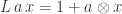
The oldest documents discovered on the third planet of the star Lambda Combinatoris (also known as the Twinkle star) talk about the prehistory of the Twinklean thought. The ancient Book of Application postulated that the Essence of Being is decomposition, expressed symbolically as
meaning that can be decomposed into and . The breakthrough came with the realization that, if itself can be decomposed
then could be further decomposed into
Similarly, if can be decomposed
then
In the latter case (but not the former), it became customary to drop the parentheses and simply write it as
Following these discoveries, the Twinklean civilization went through a period called The Great Decomposition that lasted almost three thousand years, during which essentially anything that could be decomposed was successfully decomposed.
At the end of The Great Decomposition, a new school of thought emerged, claiming that, if things can be decomposed into parts, they can be also recomposed from these parts.
Initially there was strong resistance to this idea. The argument was put forward that decomposition followed by recomposition doesn’t change anything. This was settled by the introduction of a special object called The Eye, denoted by defined by the unique property of leaving things alone
After the introduction of , a long period of general stagnation accompanied by lack of change followed.
We also don’t have many records from the next period, as it was marked by attempts at forgetting things and promoting ignorance. It started by the introduction of , which ignores one of its inputs
Notice that this definition is a shorthand for the parenthesized version
The argument for introducing was that ignorance is an important part of understanding. By rejecting we are saying that is important. We are abstracting away the inessential part .
For instance—the argument went—if we decompose
and happens to have a similar decomposition
then will abstract the part from both and . From the perspective of , there is no difference between and .
The only positive outcome of the Era of Ignorance was the development of abstract mathematics. Twinklean thinkers argued that, if you disregard the particularities of the fruit in question, there is no difference between having three apples and three oranges. Number three was thus born, followed by many others (four and seven, to name just a few).
The final Industrial phase of the Twinklean civilization that ultimately led to their demise was marked by the introduction of . The Twinklean industry was based on the principle of mass production; and mass production starts with duplication and reuse. Suppose you have a reusable part . allows you to duplicate and combine it with both and .
If you think of and as abstractions—that is the results of ignoring some parts of the whole— lets you substitute in place of those forgotten parts.
Or, conversely, it tells you that the object
can be decomposed into two parts that have something in common. This common part is .
Unfortunately, during the Industrial period, a lot of Twinkleans lost their identity. They discovered that
Indeed
But ultimately, what precipitated their end was the existential crisis. They lost their will to live because they couldn’t figure out .
Postscript
After submitting this paper to the journal of Compositionality, we have been informed by the reviewer that a similar theory of SKI combinators was independently developed on Earth by a Russian logician, Moses Schönfinkel. According to this reviewer, the answer to the meaning of life is the combinator, which introduces recursion and can be expressed as
We were unable to verify this assertion, as it led us into a rabbit hole.
This post is based on the talk I gave in Moscow, Russia, in February 2015 to an audience of C++ programmers.
Let’s agree on some preliminaries.
C++ is a low level programming language. It’s very close to the machine. C++ is engineering at its grittiest.
Category theory is the most abstract branch of mathematics. It’s very very high in the layers of abstraction. Category theory is mathematics at its highest.
So why have I decided to speak about category theory to C++ programmers? There are many reasons.
The main reason is that category theory captures the essence of programming. We can program at many levels, and if I ask somebody “What is programming?” most C++ programmers will probably say that it’s about telling the computer what to do. How to move bytes from memory to the processor, how to manipulate them, and so on.
But there is another view of programming and it’s related to the human side of programming. We are humans writing programs. We decide what to tell the computer to do.
We are solving problems. We are finding solutions to problems and translating them in the language that is understandable to the computer.
But what is problem solving? How do we, humans, approach problem solving? It was only a recent development in our evolution that we have acquired these fantastic brains of ours. For hundreds of millions of years not much was happening under the hood, and suddenly we got this brain, and we used this brain to help us chase animals, shoot arrows, find mates, organize hunting parties, and so on. It’s been going on for a few hundred thousand years. And suddenly the same brain is supposed to solve problems in software engineering.
So how do we approach problem solving? There is one general approach that we humans have developed for problem solving. We had to develop it because of the limitations of our brain, not because of the limitations of computers or our tools. Our brains have this relatively small cache memory, so when we’re dealing with a huge problem, we have to split it into smaller parts. We have to decompose bigger problems into smaller problems. And this is very human. This is what we do. We decompose, and then we attack each problem separately, find the solution; and once we have solutions to all the smaller problems, we recompose them.
So the essence of programming is composition.
If we want to be good programmers, we have to understand composition. And who knows more about composing than musicians? They are the original composers!
So let me show you an example. This is a piece by Johann Sebastian Bach. I’ll show you two versions of this composition. One is low level, and one is high level.
The low level is just sampled sound. These are bytes that approximate the waveform of the sound.
And this is the same piece in typical music notation.
Which one is easier to manipulate? Which one is easier to reason about? Obviously, the high level one!
Notice that, in the high level language, we use a lot of different abstractions that can be processed separately. We split the problem into smaller parts. We know that there are things called notes, and they can be reproduced, in this particular case, using violins. There are also some letters like E, A, B7: these are chords. They describe harmony. There is melody, there is harmony, there is the bass line.
Musicians, when they compose music, use higher level abstractions. These higher level abstractions are easier to manipulate, reason about, and modify when necessary.
And this is probably what Bach was hearing in his head.
And he chose to represent it using the high level language of musical notation.
Now, if you’re a rap musician, you work with samples, and you learn how to manipulate the low level description of music. It’s a very different process. It’s much closer to low-level C++ programming. We often do copy and paste, just like rap musicians. There’s nothing wrong with that, but sometimes we would like to be more like Bach.
So how do we approach this problem as programmers and not as musicians. We cannot use musical notation to lift ourselves to higher levels of abstraction. We have to use mathematics. And there is one particular branch of mathematics, category theory, that is exactly about composition. If programming is about composition, then this is what we should be looking at.
Category theory, in general, is not easy to learn, but the basic concepts of category theory are embarrassingly simple. So I will talk about some of those embarrassingly simple concepts from category theory, and then explain how to use them in programming in some weird ways that would probably not have occurred to you when you’re programming.
Categories
So what is this concept of a category? Two things: object and arrows between objects.
In category theory you don’t ask what these objects are. You call them objects, you give them names like A, B, C, D, etc., but you don’t ask what they are or what’s inside them. And then you have arrows that connect objects. Every arrow starts at some object and ends at some object. You can have many arrows going between two objects, or none whatsoever. Again, you don’t ask what these arrows are. You just give them names like f, g, h, etc.
And that’s it—that’s how you visualize a category: a bunch of objects and a bunch of arrows between them.
There are some operations on arrows and some laws that they have to obey, and they are also very simple.
Since composition is the essence of category theory (and of programming), we have to define composition in a category.
Whenever you have an arrow f going from object A to object B, here represented by two little piggies, and another arrow g going from object B to object C, there is an arrow called their composition, g ∘ f, that goes directly from object A to object C. We pronounce this “g after f.”
Composition is part of the definition of a category. Again, since we don’t know what these arrows are, we don’t ask what composition is. We just know that for any two composable arrows — such that the end of one coincides with the start of the other — there exists another arrow that’s their composition.
And this is exactly what we do when we solve problems. We find an arrow from A to B — that’s our subproblem. We find an arrow from B to C, that’s another subproblem. And then we compose them to get an arrow from A to C, and that’s a solution to our bigger problem. We can repeat this process, building larger and larger solutions by solving smaller problems and composing the solutions.
Notice that when we have three arrows to compose, there are two ways of doing that, depending on which pair we compose first. We don’t want composition to have history. We want to be able to say: This arrow is a composition of these three arrows: f after g after h, without having to use parentheses for grouping. That’s called associativity:
(f ∘ g) ∘ h = f ∘ (g ∘ h)
Composition in a category must be associative.
And finally, every object has to have an identity arrow. It’s an arrow that goes from the object back to itself. You can have many arrows that loop back to the same object. But there is always one such loop for every object that is the identity with respect to composition.
It has the property that if you compose it with any other arrow that’s composable with it — meaning it either starts or ends at this object — you get that arrow back. It acts like multiplication by one. It’s an identity — it doesn’t change anything.
Monoid
I can immediately give you an example of a very simple category that I’m sure you know very well and have used all your adult life. It’s called a monoid. It’s another embarrassingly simple concept. It’s a category that has only one object. It may have lots of arrows, but all these arrows have to start at this object and end at this object, so they are all composable. You can compose any two arrows in this category to get another arrow. And there is one arrow that’s the identity. When composed with any other arrow it will give you back the same arrow.
There are some very simple examples of monoids. We have natural numbers with addition and zero. An arrow corresponds to adding a number. For instance, you will have an arrow that corresponds to adding 5. You compose it with an arrow that corresponds to adding 3, and you get an arrow that corresponds to adding 8. Identity arrow corresponds to adding zero.
Multiplication forms a monoid too. The identity arrow corresponds to multiplying by 1. The composition rule for these arrows is just a multiplication table.
Strings form another interesting monoid. An arrow corresponds to appending a particular string. Unit arrow appends an empty string. What’s interesting about this monoid is that it has no additional structure. In particular, it doesn’t have an inverse for any of its arrows. There are no “negative” strings. There is no anti-“world” string that, when appended to “Hello world”, would result in the string “Hello“.
In each of these monoids, you can think of the one object as being a set: a set of all numbers, or a set of all strings. But that’s just an aid to imagination. All information about the monoid is in the composition rules — the multiplication table for arrows.
In programming we encounter monoids all over the place. We just normally don’t call them that. But every time you have something like logging, gathering data, or auditing, you are using a monoid structure. You’re basically adding some information to a log, appending, or concatenating, so that’s a monoidal operation. And there is an identity log entry that you may use when you have nothing interesting to add.
Types and Functions
So monoid is one example, but there is something closer to our hearts as programmers, and that’s the category of types and functions. And the funny thing is that this category of types and functions is actually almost enough to do programming, and in functional languages that’s what people do. In C++ there is a little bit more noise, so it’s harder to abstract this part of programming, but we do have types — it’s a strongly typed language, modulo implicit conversions. And we do have functions. So let’s see why this is a category and how it’s used in programming.
This category is actually called Set — a category of sets — because, to the lowest approximation, types are just sets of values. The type bool is a set of two values, true and false. The type int is a set of integers from something like negative two billion to two billion (on a 32-bit machine). All types are sets: whether it’s numbers, enums, structs, or objects of a class. There could be an infinite set of possible values, but it’s okay — a set may be infinite. And functions are just mappings between these sets. I’m talking about the simplest functions, ones that take just one value of some type and return another value of another type. So these are arrows from one type to another.
Can we compose these functions? Of course we can. We do it all the time. We call one function, it returns some value, and with this value we call another function. That’s function composition. In fact this is the basis of procedural decomposition, the first serious approach to formalizing problem solving in programming.
Here’s a piece of C++ code that composes two functions f and g.
C g_after_f(A x) {
    B y = f(x);
    return g(y);
}
In modern C++ you can make this code generic — a higher order function that accepts two functions and returns a third function that’s the composition of the two.
Can you compose any two functions? Yes — if they are composable. The output type of one must match the input type of another. That’s the essence of strong typing in C++ (modulo implicit conversions).
Is there an identity function? Well, in C++ we don’t have an identity function in the library, which is too bad. That’s because there’s a complex issue of how you pass things: is it by value, by reference, by const reference, by move, and so on. But in functional languages there is just one function called identity. It takes an argument and returns it back. But even in C++, if you limit yourself to functions that take arguments by value and return values, then it’s very easy to define a generic identity function.
Notice that the functions I’m talking about are actually special kind of functions called pure functions. They can’t have any side effects. Mathematically, a function is just a mapping from one set to another set, so it can’t have side effects. Also, a pure function must return the same value when called with the same arguments. This is called referential transparency.
A pure function doesn’t have any memory or state. It doesn’t have static variables, and doesn’t use globals. A pure function is an ideal we strive towards in programming, especially when writing reusable components and libraries. We don’t like having global variables, and we don’t like state hidden in static variables.
Moreover, if a function is pure, you can memoize it. If a function takes a long time to evaluate, maybe you’ll want to cache the value, so it can be retrieved quickly next time you call it with the same arguments.
Another property of pure functions is that all dependencies in your code only come through composition. If the result of one function is used as an argument to another then obviously you can’t run them in parallel or reverse the order of execution. You have to call them in that particular order. You have to sequence their execution. The dependencies between functions are fully explicit. This is not true for functions that have side effects. They may look like independent functions, but they have to be executed in sequence, or their side effects will be different.
We know that compiler optimizers will try to rearrange our code, but it’s very hard to do it in C++ because of hidden dependencies. If you have two functions that are not composed, they just calculate different things, and you try to call them in a different order, you might get a completely different result. It’s because of the order of side effects, which are invisible to the compiler. You would have to go deep into the implementation of the functions; you would have to analyse everything they are doing, and the functions they are calling, and so on, in order to find out what these side effects are; and only then you could decide: Oh, I can swap these two functions.
In functional programming, where you only deal with pure functions, you can swap any two functions that are not explicitly composed, and composition is immediately visible.
At this point I would expect half of the audience to leave and say: “You can’t program with pure functions, Programming is all about side effects.” And it’s true. So in order to keep you here I will have to explain how to deal with side effects. But it’s important that you start with something that is easy to understand, something you can reason about, like pure functions, and then build side effects on top of these things, so you can build up abstractions on top of other abstractions.
You start with pure functions and then you talk about side effects, not the other way around.
Auditing
Instead of explaining the general theory of side effects in category theory, I’ll give you an example from programming. Let’s solve this simple problem that, in all likelihood, most C++ programmers would solve using side effects. It’s about auditing.
You start with a sequence of functions that you want to compose. For instance, you have a function getKey. You give it a password and it returns a key. And you have another function, withdraw. You give it a key and gives you back money. You want to compose these two functions, so you start with a password and you get money. Excellent!
But now you have a new requirement: you want to have an audit trail. Every time one of these functions is called, you want to log something in the audit trail, so that you’ll know what things have happened and in what order. That’s a side effect, right?
How do we solve this problem? Well, how about creating a global variable to store the audit trail? That’s the simplest solution that comes to mind. And it’s exactly the same method that’s used for standard output in C++, with the global object std::cout. The functions that access a global variable are obviously not pure functions, we are talking about side effects.
So we have a string, audit, it’s a global variable, and in each of these functions we access this global variable and append something to it. For simplicity, I’m just returning some fake numbers, not to complicate things.
This is not a good solution, for many reasons. It doesn’t scale very well. It’s difficult to maintain. If you want to change the name of the variable, you’d have to go through all this code and modify it. And if, at some point, you decide you want to log more information, not just a string but maybe a timestamp as well, then you have to go through all this code again and modify everything. And I’m not even mentioning concurrency. So this is not the best solution.
But there is another solution that’s really pure. It’s based on the idea that whatever you’re accessing in a function, you should pass explicitly to it, and then return it, with modifications, from the function. That’s pure. So here’s the next solution.
You modify all the functions so that they take an additional argument, the audit string. And the return type is also changed. When we had an int before, it’s now a pair of int and string. When we had a double before, it’s now a pair of double and string. These function now call make_pair before they return, and they put in whatever they were returning before, plus they do this concatenation of a new message at the end of the old audit string. This is a better solution because it uses pure functions. They only depend on their arguments. They don’t have any state, they don’t access any global variables. Every time you call them with the same arguments, they produce the same result.
The problem though is that they don’t memoize that well. Look at the function logIn: you normally get the same key for the same password. But if you want to memoize it when it takes two arguments, you suddenly have to memoize it for all possible histories. Even if you call it with the same password, but the audit string is different, you can’t just access the cache, you have to cache a new pair of values. Your cache explodes with all possible histories.
An even bigger problem is security. Each of these functions has access to the complete log, including the passwords.
Also, each of these functions has to care about things that maybe it shouldn’t be bothered with. It knows about how to concatenate strings. It knows the details of the implementation of the log: that the log is a string. It must know how to accumulate the log.
Now I want to show you a solution that maybe is not that obvious, maybe a little outside of what we would normally think of.
We use modified functions, but they don’t take the audit string any more. They just return a pair of whatever they were returning before, plus a string. But each of them only creates a message about what it considers important. It doesn’t have access to any log and it doesn’t know how to work with an audit trail. It’s just doing its local thing. It’s only responsible for its local data. It’s not responsible for concatenation.
It still creates a pair and it has a modified return type.
We have one problem though: we don’t know how to compose these functions. We can’t pass a pair of key and string from logIn to withdraw, because withdraw expects an int. Of course we could extract the int and drop the string, but that would defeat the goal of auditing the code.
Let’s go back a little bit and see how we can abstract this thing. We have functions that used to return some types, and now they return pairs of the original type and a string. This should in principle work with any original type, not just an int or a double. In functional programming we call this “lifting.” Here we lift some type A to a new type, which is a pair of A and a string. Or we can say that we are “embellishing” the return type of a function by pairing it with a string.
I’ll create an alias for this new parameterised type and call it Writer.
template<class A>
using Writer = pair<A, string>;
My functions now return Writers: logIn returns a writer of int, and withdraw returns a writer of double. They return “embellished” types.
In this case we want to compose logIn with withdraw to create a new function called transact. This new function transact will take a password, log the user in, withdraw money, and return the money plus the audit trail. But it will return the audit trail only from those two functions.
Writer<double> transact(string passwd){
  auto p1 logIn(passwd);
  auto p2 withdraw(p1.first);
  return make_pair(p2.first
          , p1.second + p2.second);
}
How is it done? It’s very simple. I call the first function, logIn, with the password. It returns a pair of key and string. Then I call the second function, passing it the first component of the pair — the key. I get a new pair with the money and a string. And then I perform the composition. I take the money, which is the first component of the second pair, and I pair it with the concatenation of the two string that were the second components of the pairs returned by logIn and withdraw.
So the accumulation of the log is done “in between” the calls (think of composition as happening between calls). I have these two functions, and I’m composing them in this funny way that involves the concatenation of strings. The accumulation of the log does not happen inside these two functions, as it happened before. It happens outside. And I can pull out this code and abstract the composition. It doesn’t really matter what functions I’m calling. I can do it for any two functions that return embellished results. I can write generic code that does it and I can call it “compose”.
template<class A, class B, class C>
function<Writer<C>(A)> compose(function<Writer<B>(A)> f
                              ,function<Writer<C>(B)> g)
{
    return [f, g](A x) {
        auto p1 = f(x);
        auto p2 = g(p1.first);
        return make_pair(p2.first
                  , p1.second + p2.second);
    };
}
What does compose do? It takes two functions. The first function takes A and returns a Writer of B. The second function takes a B and return a Writer of C. When I compose them, I get a function that takes an A and returns a Writer of C.
This higher order function just does the composition. It has no idea that there are functions like logIn or withdraw, or any other functions that I may come up with later. It takes two embellished functions and glues them together.
We’re lucky that in modern C++ we can work with higher order functions that take functions as arguments and return other functions.
This is how I would implement the transact function using compose.
The transact function is nothing but the composition of logIn and withdraw. It doesn’t contain any other logic. I’m using this special composition because I want to create an audit trail. And the audit trail is accumulated “between” the calls — it’s in the glue that glues these two functions together.
This particular implementation of compose requires explicit type annotations, which is kind of ugly. We would like the types to be inferred. And you can do it in C++14 using generalised lambdas with return type deduction. This code was contributed by Eric Niebler.
auto const compose = [](auto f, auto g) {
    return [f, g](auto x) {
        auto p1 = f(x);
        auto p2 = g(p1.first);
        return make_pair(p2.first
                    , p1.second + p2.second);
    };
};
Now that we’ve done this example, let’s go back to where we started. In category theory we have functions and we have composition of functions. Here we also have functions and composition, but it’s a funny composition. We have functions that take simple types, but they return embellished types. The types don’t match.
Let me remind you what we had before. We had a category of types and pure functions with the obvious composition.
Objects: types,
Arrows: pure functions,
Composition: pass the result of one function as the argument to another.
What we have created just now is a different category. Slightly different. It’s a category of embellished functions. Objects are still types: Types A, B, C, like integers, doubles, strings, etc. But an arrow from A to B is not a function from type A to type B. It’s a function from type A to the embellishment of the type B. The embellished type depends on the type B — in our case it was a pair type that combined B and a string — the Writer of B.
Now we have to say how to compose these arrows. It’s not as trivial as it was before. We have one arrow that takes A into a pair of B and string, and we have another arrow that takes B into a pair of C and string, and the composition should take an A and return a pair of C and string. And I have just defined this composition. I wrote code that does this:
auto const compose = [](auto f, auto g) {
    return [f, g](auto x) {
        auto p1 = f(x);
        auto p2 = g(p1.first);
        return make_pair(p2.first
                    , p1.second + p2.second);
    };
};
So do we have a category here? A category that’s different from the original category? Yes, we do! It has composition and it has identity.
What’s its identity? It has to be an arrow from the object to itself, from A to A. But an arrow from A to A is a function from A to a pair of A and string — to a Writer of A. Can we implement something like this? Yes, easily. We will return a pair that contains the original value and the empty string. The empty string will not contribute to our audit trail.
template<class A>
Writer<A> identity(A x) {
    return make_pair(x, "");
}
Is this composition associative? Yes, it is, because the underlying composition is associative, and the concatenation of strings is associative.
We have a new category. We have incorporated side effects by modifying the original category. We are still only using pure functions and yet we are able to accumulate an audit trail as a side effect. And we moved the side effects to the definition of composition.
It’s a funny new way of looking at programming. We usually see the functions, and the data being passed between functions, and here suddenly we see a new dimension to programming that is orthogonal to this, and we can manipulate it. We change the way we compose functions. We have this new power to change composition. We have a new way of solving problems by moving to these embellished functions and defining a new way of composing them. We can define new combinators to compose functions, and we’ll let the combinators do some work that we don’t want these functions to do. We can factor these things out and make them orthogonal.
Does this approach generalize?
One easy generalisation is to observe that the Writer structure works for any monoid. It doesn’t have to be just strings. Look at how composition and identity are defined in our new cateogory. The only properties of the log we are using are concatenation and unit. Concatenation must be associative for the composition to be associative. And we need a unit of concatenation so that we can define identity in our category. We don’t need anything else. This construction will work with any monoid.
And that’s great because you have one more dimension in which you can modify your code without touching the rest. You can change the format of the log, and all you need to modify in your code is compose and identity. You don’t have to go through all your functions and modify the code. They will still work because all the concatenation of logs is done inside compose.
Kleisli Categories
This was just a little taste of what is possible with category theory. The thing I called embellishment is called a functor in category theory. You can implement categorical functors in C++. There are all kinds of embellishments/functors that you can use here. And now I can tell you the secret: this funny composition of functions with the funny identity is really a monad in disguise. A monad is just a funny way of composing embellished functions so that they form a category. A category based on a monad is called a Kleisli category.
Are there any other interesting monads that I can use this construction with? Yes, lots! I’ll give you one example. Functions that return futures. That’s our new embellishment. Give me any type A and I will embellish it by making it into a future. This embellishment also produces a Kleisli category. The composition of functions that return futures is done through the combinator “then”. You call one function returning a future and compose it with another function returning a future by passing it to “then.” You can compose these function into chains without ever having to block for a thread to finish. And there is an identity, which is a function that returns a trivial future that’s always ready. It’s called make_ready_future. It’s an arrow that takes A and returns a future of A.
Now you understand what’s really happening. We are creating this new category based on future being a monad. We have new words to describe what we are doing. We are reusing an idea from category theory to solve a completely different problem.
Resumable Functions
There is one little invonvenience with this approach. It requires writing a lot of so called “boilerplate” code. Repetitive code that obscures the simple logic. Here it’s the glue code, the “compose” and the “then.” What you’d like to do is to write your code directly in terms of embellished function, and the composition to be implicit. People noticed this and came up with solutions. In case of futures, the practical solution is called resumable functions.
Resumable functions are designed to hide the composition of functions that return futures. Here’s an example.
int cnt = 0;
do
{
   cnt = await streamR.read(512, buf);
   if ( cnt == 0 ) break;
   cnt = await streamW.write(cnt, buf);
} while (cnt > 0);
This code copies a file using a buffer, but it does it asynchronously. We call a function read that’s asynchronous. It doesn’t immediately fill the buffer, it returns a future instead. Then we call the function write that’s also asynchronous. We do it in a loop.
This code looks almost like sequential code, except that it has these await keywords. These are the points of insertion of our composition. These are the places where the code is chopped into pieces and composed using then.
I won’t go into details of the implementation. The point is that the composition of these embellished functions is almost entirely hidden. It doesn’t look like composition in a Kleisli category, but it really is.
This solution is usually described at a very low level, in terms of coroutines implemented as state machines with static variables and gotos. And what is being lost in all this engineering talk is how general this idea is — the idea of overloading composition to build a category of embellished functions.
Just to drive this home, here’s an example of different code that does completely different stuff. It calculates Fibonacci numbers on demand. It’s a generator of Fibonacci numbers.
generator<int> fib()
{
    int a = 0;
    int b = 1;
    for (;;) {
        __yield_value a;
        auto next = a + b;
        a = b;
        b = next;
    }
}
Instead of await it has __yield_value. But it’s the same idea of resumable functions, only with a different monad. This monad is called a list monad. And this kind of code in combination with Eric Niebler’s proposed range library could lead to very powerful programming idioms.
Conclusion
Why do we have to separate the two notions: that of resumable functions and that of generators, if they are based on the same abstraction? Why do we have to reinvent the wheel?
There’s this great opportunity for C++, and I’m afraid it will be missed like so many other opportunities for great generalisations that were missed in the past. It’s the opportunity to introduce one general solution based on monads, rather than keep creating ad-hoc solutions, one problem at a time. The same very general pattern can be used to control all kinds of side effects. It can be used for auditing, exceptions, ranges, futures, I/O, continuations, and all kinds of user-defined monads.
This amazing power could be ours if we start thinking in more abstract terms, if we reach into category theory.
This piece of code is probably unreadable to a regular C++ programmer, but makes perfect sense to a Haskell programmer.
Here’s the description of the problem: You are given a list of equal-length strings. Every string is different, but two of these strings differ only by one character. Find these two strings and return their matching part. For instance, if the two strings were “abcd” and “abxd”, you would return “abd”.
What makes this problem particularly interesting is its potential application to a much more practical task of matching strands of DNA while looking for mutations. I decided to explore the problem a little beyond the brute force approach. And, of course, I had a hunch that I might encounter my favorite wild beast–the hylomorphism.
Brute force approach
First things first. Let’s do the boring stuff: read the file and split it into lines, which are the strings we are supposed to process. So here it is:
main = do
  txt <- readFile "day2.txt"
  let cs = lines txt
  print $ findMatch cs
The real work is done by the function findMatch, which takes a list of strings and produces the answer, which is a single string.
findMatch :: [String] -> String
First, let’s define a function that calculates the distance between any two strings.
distance :: (String, String) -> Int
We’ll define the distance as the count of mismatched characters.
Here’s the idea: We have to compare strings (which, let me remind you, are of equal length) character by character. Strings are lists of characters. The first step is to take two strings and zip them together, producing a list of pairs of characters. In fact we can combine the zipping with the next operation–in this case, comparison for inequality, (/=)–using the library function zipWith. However, zipWith is defined to act on two lists, and we will want it to act on a pair of lists–a subtle distinction, which can be easily overcome by applying uncurry:
uncurry :: (a -> b -> c) -> ((a, b) -> c)
which turns a function of two arguments into a function that takes a pair. Here’s how we use it:
uncurry (zipWith (/=))
The comparison operator (/=) produces a Boolean result, True or False. We want to count the number of differences, so we’ll covert True to one, and False to zero:
fromBool :: Num a => Bool -> a
fromBool False = 0
fromBool True  = 1
(Notice that such subtleties as the difference between Bool and Int are blisfully ignored in C++.)
Finally, we’ll sum all the ones using sum. Altogether we have:
distance = sum . fmap fromBool . uncurry (zipWith (/=))
Now that we know how to find the distance between any two strings, we’ll just apply it to all possible pairs of strings. To generate all pairs, we’ll use list comprehension:
let ps = [(s1, s2) | s1 <- ss, s2 <- ss]
(In C++ code, this was done by cartesian_product.)
Our goal is to find the pair whose distance is exactly one. To this end, we’ll apply the appropriate filter:
filter ((== 1) . distance) ps
For our purposes, we’ll assume that there is exactly one such pair (if there isn’t one, we are willing to let the program fail with a fatal exception).
(s, s') = head $ filter ((== 1) . distance) ps
The final step is to remove the mismatched character:
filter (uncurry (==)) $ zip s s'
We use our friend uncurry again, because the equality operator (==) expects two arguments, and we are calling it with a pair of arguments. The result of filtering is a list of identical pairs. We’ll fmap fst to pick the first components.
findMatch :: [String] -> String
findMatch ss =
  let ps = [(s1, s2) | s1 <- ss, s2 <- ss]
      (s, s') = head $ filter ((== 1) . distance) ps
  in fmap fst $ filter (uncurry (==)) $ zip s s'
This program produces the correct result and we could stop right here. But that wouldn’t be much fun, would it? Besides, it’s possible that other algorithms could perform better, or be more flexible when applied to a more general problem.
Data-driven approach
The main problem with our brute-force approach is that we are comparing everything with everything. As we increase the number of input strings, the number of comparisons grows like a factorial. There is a standard way of cutting down on the number of comparison: organizing the input into a neat data structure.
We are comparing strings, which are lists of characters, and list comparison is done recursively. Assume that you know that two strings share a prefix. Compare the next character. If it’s equal in both strings, recurse. If it’s not, we have a single character fault. The rest of the two strings must now match perfectly to be considered a solution. So the best data structure for this kind of algorithm should batch together strings with equal prefixes. Such a data structure is called a prefix tree, or a trie (pronounced try).
At every level of our prefix tree we’ll branch based on the current character (so the maximum branching factor is, in our case, 26). We’ll record the character, the count of strings that share the prefix that led us there, and the child trie storing all the suffixes.
data Trie = Trie [(Char, Int, Trie)]
  deriving (Show, Eq)
Here’s an example of a trie that stores just two strings, “abcd” and “abxd”. It branches after b.
   a 2
   b 2
c 1    x 1
d 1    d 1
When inserting a string into a trie, we recurse both on the characters of the string and the list of branches. When we find a branch with the matching character, we increment its count and insert the rest of the string into its child trie. If we run out of branches, we create a new one based on the current character, give it the count one, and the child trie with the rest of the string:
insertS :: Trie -> String -> Trie
insertS t "" = t
insertS (Trie bs) s = Trie (inS bs s)
  where
    inS ((x, n, t) : bs) (c : cs) =
      if c == x
      then (c, n + 1, insertS t cs) : bs
      else (x, n, t) : inS bs (c : cs)
    inS [] (c : cs) = [(c, 1, insertS (Trie []) cs)]
We convert our input to a trie by inserting all the strings into an (initially empty) trie:
Of course, there are many optimizations we could use, if we were to run this algorithm on big data. For instance, we could compress the branches as is done in radix trees, or we could sort the branches alphabetically. I won’t do it here.
I won’t pretend that this implementation is simple and elegant. And it will get even worse before it gets better. The problem is that we are dealing explicitly with recursion in multiple dimensions. We recurse over the input string, the list of branches at each node, as well as the child trie. That’s a lot of recursion to keep track of–all at once.
Now brace yourself: We have to traverse the trie starting from the root. At every branch we check the prefix count: if it’s greater than one, we have more than one string going down, so we recurse into the child trie. But there is also another possibility: we can allow to have a mismatch at the current level. The current characters may be different but, since we allow only one mismatch, the rest of the strings have to match exactly. That’s what the function exact does. Notice that exact t is used inside foldMap, which is a version of fold that works on monoids–here, on strings.
match1 :: Trie -> [String]
match1 (Trie bs) = go bs
  where
    go :: [(Char, Int, Trie)] -> [String]
    go ((x, n, t) : bs) =
      let a1s = if n > 1
                then fmap (x:) $ match1 t
                else []
          a2s = foldMap (exact t) bs
          a3s = go bs -- recurse over list
      in a1s ++ a2s ++ a3s
    go [] = []
    exact t (_, _, t') = matchAll t t'
Here’s the function that finds all exact matches between two tries. It does it by generating all pairs of branches in which top characters match, and then recursing down.
When mAll reaches the leaves of the trie, it returns a singleton list containing an empty string. Subsequent actions of fmap (c:) will prepend characters to this string.
Since we are expecting exactly one solution to the problem, we’ll extract it using head:
As you hone your functional programming skills, you realize that explicit recursion is to be avoided at all cost. There is a small number of recursive patterns that have been codified, and they can be used to solve the majority of recursion problems (for some categorical background, see F-Algebras). Recursion itself can be expressed in Haskell as a data structure: a fixed point of a functor:
newtype Fix f = In { out :: f (Fix f) }
In particular, our trie can be generated from the following functor:
data TrieF a = TrieF [(Char, a)]
  deriving (Show, Functor)
Notice how I have replaced the recursive call to the Trie type constructor with the free type variable a. The functor in question defines the structure of a single node, leaving holes marked by the occurrences of a for the recursion. When these holes are filled with full blown tries, as in the definition of the fixed point, we recover the complete trie.
I have also made one more simplification by getting rid of the Int in every node. This is because, in the recursion scheme I’m going to use, the folding of the trie proceeds bottom-up, rather than top-down, so the multiplicity information can be passed upwards.
The main advantage of recursion schemes is that they let us use simpler, non-recursive building blocks such as algebras and coalgebras. Let’s start with a simple coalgebra that lets us build a trie from a list of strings. A coalgebra is a fancy name for a particular type of function:
type Coalgebra f x = x -> f x
Think of x as a type for a seed from which one can grow a tree. A colagebra tells us how to use this seed to create a single node described by the functor f and populate it with (presumably smaller) seeds. We can then pass this coalgebra to a simple algorithm, which will recursively expand the seeds. This algorithm is called the anamorphism:
ana :: Functor f => Coalgebra f a -> a -> Fix f
ana coa = In . fmap (ana coa) . coa
Let’s see how we can apply it to the task of building a trie. The seed in our case is a list of strings (as per the definition of our problem, we’ll assume they are all equal length). We start by grouping these strings into bunches of strings that start with the same character. There is a library function called groupWith that does exactly that. We have to import the right library:
import GHC.Exts (groupWith)
This is the signature of the function:
groupWith :: Ord b => (a -> b) -> [a] -> [[a]]
It takes a function a -> b that converts each list element to a type that supports comparison (as per the typeclass Ord), and partitions the input into lists that compare equal under this particular ordering. In our case, we are going to extract the first character from a string using head and bunch together all strings that share that first character.
let sss = groupWith head ss
The tails of those strings will serve as seeds for the next tier of the trie. Eventually the strings will be shortened to nothing, triggering the end of recursion.
fromList :: Coalgebra TrieF [String]
fromList ss =
  -- are strings empty? (checking one is enough)
  if null (head ss)
  then TrieF [] -- leaf
  else
    let sss = groupWith head ss
    in TrieF $ fmap mkBranch sss
The function mkBranch takes a bunch of strings sharing the same first character and creates a branch seeded with the suffixes of those strings.
mkBranch :: [String] -> (Char, [String])
mkBranch sss =
  let c = head (head sss) -- they're all the same
  in (c, fmap tail sss)
Notice that we have completely avoided explicit recursion.
The next step is a little harder. We have to fold the trie. Again, all we have to define is a step that folds a single node whose children have already been folded. This step is defined by an algebra:
type Algebra f x = f x -> x
Just as the type x described the seed in a coalgebra, here it describes the accumulator–the result of the folding of a recursive data structure.
We pass this algebra to a special algorithm called a catamorphism that takes care of the recursion:
cata :: Functor f => Algebra f a -> Fix f -> a
cata alg = alg . fmap (cata alg) . out
Notice that the folding proceeds from the bottom up: the algebra assumes that all the children have already been folded.
The hardest part of designing an algebra is figuring out what information needs to be passed up in the accumulator. We obviously need to return the final result which, in our case, is the list of strings with one mismatched character. But when we are in the middle of a trie, we have to keep in mind that the mismatch may still happen above us. So we also need a list of strings that may serve as suffixes when the mismatch occurs. We have to keep them all, because they might be matched later with strings from other branches.
In other words, we need to be accumulating two lists of strings. The first list accumulates all suffixes for future matching, the second accumulates the results: strings with one mismatch (after the mismatch has been removed). We therefore should implement the following algebra:
Algebra TrieF ([String], [String])
To understand the implementation of this algebra, consider a single node in a trie. It’s a list of branches, or pairs, whose first component is the current character, and the second a pair of lists of strings–the result of folding a child trie. The first list contains all the suffixes gathered from lower levels of the trie. The second list contains partial results: strings that were matched modulo single-character defect.
As an example, suppose that you have a node with two branches:
This way we convert each branch to a pair of lists.
[ (["abcd", "aefg"], ["apq"])
, (["xbcd"],         [])]
We then merge all the lists of suffixes and, separately, all the lists of partial results, across all branches. In the example above, we concatenate the lists in the two columns.
(["abcd", "aefg", "xbcd"], ["apq"])
Now we have to construct new partial results. To do this, we create another list of accumulated strings from all branches (this time without prefixing them):
ss = concat $ fmap (fst . snd) bs
In our case, this would be the list:
["bcd", "efg", "bcd"]
To detect duplicate strings, we’ll insert them into a multiset, which we’ll implement as a map. We need to import the appropriate library:
import qualified Data.Map as M
and define a multiset Counts as:
type Counts a = M.Map a Int
Every time we add a new item, we increment the count:
add :: Ord a => Counts a -> a -> Counts a
add cs c = M.insertWith (+) c 1 cs
To insert all strings from a list, we use a fold:
mset = foldl add M.empty ss
We are only interested in items that have multiplicity greater than one. We can filter them and extract their keys:
dups = M.keys $ M.filter (> 1) mset
Here’s the complete algebra:
accum :: Algebra TrieF ([String], [String])
accum (TrieF []) = ([""], [])
accum (TrieF bs) = -- b :: (Char, ([String], [String]))
    let -- prepend chars to string in both lists
        pss = unzip $ fmap prep bs
        (ss1, ss2) = both concat pss
        -- find duplicates
        ss = concat $ fmap (fst . snd) bs
        mset = foldl add M.empty ss
        dups = M.keys $ M.filter (> 1) mset
     in (ss1, dups ++ ss2)
  where
      prep :: (Char, ([String], [String])) -> ([String], [String])
      prep (c, pss) = both (fmap (c:)) pss
I used a handy helper function that applies a function to both components of a pair:
both :: (a -> b) -> (a, a) -> (b, b)
both f (x, y) = (f x, f y)
And now for the grand finale: Since we create the trie using an anamorphism only to immediately fold it using a catamorphism, why don’t we cut the middle person? Indeed, there is an algorithm called the hylomorphism that does just that. It takes the algebra, the coalgebra, and the seed, and returns the fully charged accumulator.
hylo :: Functor f => Algebra f a -> Coalgebra f b -> b -> a
hylo alg coa = alg . fmap (hylo alg coa) . coa
And this is how we extract and print the final result:
print $ head $ snd $ hylo accum fromList cs
Conclusion
The advantage of using the hylomorphism is that, because of Haskell’s laziness, the trie is never wholly constructed, and therefore doesn’t require large amounts of memory. At every step enough of the data structure is created as is needed for immediate computation; then it is promptly released. In fact, the definition of the data structure is only there to guide the steps of the algorithm. We use a data structure as a control structure. Since data structures are much easier to visualize and debug than control structures, it’s almost always advantageous to use them to drive computation.
In fact, you may notice that, in the very last step of the computation, our accumulator recreates the original list of strings (actually, because of laziness, they are never fully reconstructed, but that’s not the point). In reality, the characters in the strings are never copied–the whole algorithm is just a choreographed dance of internal pointers, or iterators. But that’s exactly what happens in the original C++ algorithm. We just use a higher level of abstraction to describe this dance.
I haven’t looked at the performance of various implementations. Feel free to test it and report the results. The code is available on github.
Acknowledgments
I’m grateful to the participants of the Seattle Haskell Users’ Group for many helpful comments during my presentation.
There is a lot of folklore about various data types that pop up in discussions about lenses. For instance, it’s known that FunList and Bazaar are equivalent, although I haven’t seen a proof of that. Since both data structures appear in the context of Traversable, which is of great interest to me, I decided to do some research. In particular, I was interested in translating these data structures into constructs in category theory. This is a continuation of my previous blog posts on free monoids and free applicatives. Here’s what I have found out:
FunList is a free applicative generated by the Store functor. This can be shown by expressing the free applicative construction using Day convolution.
Using Yoneda lemma in the category of applicative functors I can show that Bazaar is equivalent to FunList
Let’s start with some definitions. FunList was first introduced by Twan van Laarhoven in his blog. Here’s a (slightly generalized) Haskell definition:
data FunList a b t = Done t
                   | More a (FunList a b (b -> t))
It’s a non-regular inductive data structure, in the sense that its data constructor is recursively called with a different type, here the function type b->t. FunList is a functor in t, which can be written categorically as:
where is a shorthand for the hom-set .
Strictly speaking, a recursive data structure is defined as an initial algebra for a higher-order functor. I will show that the higher order functor in question can be written as:
where is the (indexed) store comonad, which can be written as:
Here, is the constant functor, and is the hom-functor. In Haskell, this is equivalent to:
newtype Store a b s = Store (a, b -> s)
The standard (non-indexed) Store comonad is obtained by identifying a with b and it describes the objects of the slice category (morphisms are functions that make the obvious triangles commute).
If you’ve read my previous blog posts, you may recognize in the functor that generates a free applicative functor (or, equivalently, a free monoidal functor). Its fixed point can be written as:
The star stands for Day convolution–in Haskell expressed as an existential data type:
data Day f g s where
  Day :: f a -> g b -> ((a, b) -> s) -> Day f g s
Intuitively, is a “list of” Store functors concatenated using Day convolution. An empty list is the identity functor, a one-element list is the Store functor, a two-element list is the Day convolution of two Store functors, and so on…
In Haskell, we would express it as:
data FunList a b t = Done t
                   | More ((Day (Store a b) (FunList a b)) t)
To show the equivalence of the two definitions of FunList, let’s expand the definition of Day convolution inside :
The coend corresponds, in Haskell, to the existential data type we used in the definition of Day.
Since we have the hom-functor under the coend, the first step is to use the co-Yoneda lemma to “perform the integration” over , which replaces with everywhere. We get:
We can then evaluate the constant functor and use the currying adjunction:
to get:
Applying the co-Yoneda lemma again, we replace with :
This is exactly the functor that generates FunList. So FunList is indeed the free applicative generated by Store.
All transformations in this derivation were natural isomorphisms.
Now let’s switch our attention to Bazaar, which can be defined as:
type Bazaar a b t = forall f. Applicative f => (a -> f b) -> f t
(The actual definition of Bazaar in the lens library is even more general–it’s parameterized by a profunctor in place of the arrow in a -> f b.)
The universal quantification in the definition of Bazaar immediately suggests the application of my favorite double Yoneda trick in the functor category: The set of natural transformations (morphisms in the functor category) between two functors (objects in the functor category) is isomorphic, through Yoneda embedding, to the following end in the functor category:
The end is equivalent (modulo parametricity) to Haskell forall. Here, the sets of natural transformations between pairs of functors are just hom-functors in the functor category and the end over is a set of higher-order natural transformations between them.
In the double Yoneda trick we carefully select the two functors and to be either representable, or somehow related to representables.
The universal quantification in Bazaar is limited to applicative functors, so we’ll pick our two functors to be free applicatives. We’ve seen previously that the higher-order functor that generates free applicatives has the form:
Here’s the version of the Yoneda embedding in which varies over all applicative functors in the category , and and are arbitrary functors in :
The free functor is the left adjoint to the forgetful functor :
Using this adjunction, we arrive at:
We’re almost there–we just need to carefuly pick the functors and . In order to arrive at the definition of Bazaar we want:
The right hand side becomes:
where I represented natural transformations as ends. The first term can be curried:
and the end over can be evaluated using the Yoneda lemma. So can the second term. Altogether, the right hand side becomes:
In Haskell notation, this is just the definition of Bazaar:
forall f. Applicative f => (a -> f b) -> f t
The left hand side can be written as:
Since we have chosen to be the hom-functor , we can use the Yoneda lemma to “perform the integration” and arrive at:
With our choice of , this is exactly the free applicative generated by Store–in other words, FunList.
This proves the equivalence of Bazaar and FunList. Notice that this proof is only valid for -valued functors, although a generalization to the enriched setting is relatively straightforward.
There is another family of functors, Traversable, that uses universal quantification over applicatives:
class (Functor t, Foldable t) => Traversable t where
  traverse :: forall f. Applicative f => (a -> f b) -> t a -> f (t b)
The same double Yoneda trick can be applied to it to show that it’s related to Bazaar. There is, however, a much simpler derivation, suggested to me by Derek Elkins, by changing the order of arguments:
traverse :: t a -> (forall f. Applicative f => (a -> f b) -> f (t b))
which is equivalent to:
traverse :: t a -> Bazaar a b (t b)
In view of the equivalence between Bazaar and FunList, we can also write it as:
traverse :: t a -> FunList a b (t b)
Note that this is somewhat similar to the definition of toList:
toList :: Foldable t => t a -> [a]
In a sense, FunList is able to freely accumulate the effects from traversable, so that they can be interpreted later.
Acknowledgments
I’m grateful to Edward Kmett and Derek Elkins for many discussions and valuable insights.
The use of free monads, free applicatives, and cofree comonads lets us separate the construction of (often effectful or context-dependent) computations from their interpretation. In this paper I show how the ad hoc process of writing interpreters for these free constructions can be systematized using the language of higher order algebras (coalgebras) and catamorphisms (anamorphisms).
Introduction
Recursive schemes [meijer] are an example of successful application of concepts from category theory to programming. The idea is that recursive data structures can be defined as initial algebras of functors. This allows a separation of concerns: the functor describes the local shape of the data structure, and the fixed point combinator builds the recursion. Operations over data structures can be likewise separated into shallow, non-recursive computations described by algebras, and generic recursive procedures described by catamorphisms. In this way, data structures often replace control structures in driving computations.
Since functors also form a category, it’s possible to define functors acting on functors. Such higher order functors show up in a number of free constructions, notably free monads, free applicatives, and cofree comonads. These free constructions have good composability properties and they provide means of separating the creation of effectful computations from their interpretation.
This paper’s contribution is to systematize the construction of such interpreters. The idea is that free constructions arise as fixed points of higher order functors, and therefore can be approached with the same algebraic machinery as recursive data structures, only at a higher level. In particular, interpreters can be constructed as catamorphisms or anamorphisms of higher order algebras/coalgebras.
Initial Algebras and Catamorphisms
The canonical example of a data structure that can be described as an initial algebra of a functor is a list. In Haskell, a list can be defined recursively:
data List a = Nil | Cons a (List a)
There is an underlying non-recursive functor:
data ListF a x = NilF | ConsF a x
instance Functor (ListF a) where
  fmap f NilF = NilF
  fmap f (ConsF a x) = ConsF a (f x)
Once we have a functor, we can define its algebras. An algebra consist of a carrier c and a structure map (evaluator). An algebra can be defined for an arbitrary functor f:
type Algebra f c = f c -> c
Here’s an example of a simple list algebra, with Int as its carrier:
sum :: Algebra (ListF Int) Int
sum NilF = 0
sum (ConsF a c) = a + c
Algebras for a given functor form a category. The initial object in this category (if it exists) is called the initial algebra. In Haskell, we call the carrier of the initial algebra Fix f. Its structure map is a function:
f (Fix f) -> Fix f
By Lambek’s lemma, the structure map of the initial algebra is an isomorphism. In Haskell, this isomorphism is given by a pair of functions: the constructor In and the destructor out of the fixed point combinator:
newtype Fix f = In { out :: f (Fix f) }
When applied to the list functor, the fixed point gives rise to an alternative definition of a list:
type List a = Fix (ListF a)
The initiality of the algebra means that there is a unique algebra morphism from it to any other algebra. This morphism is called a catamorphism and, in Haskell, can be expressed as:
cata :: Functor f => Algebra f a -> Fix f -> a
cata alg = alg . fmap (cata alg) . out
A list catamorphism is known as a fold. Since the list functor is a sum type, its algebra consists of a value—the result of applying the algebra to NilF—and a function of two variables that corresponds to the ConsF constructor. You may recognize those two as the arguments to foldr:
foldr :: (a -> c -> c) -> c -> [a] -> c
The list functor is interesting because its fixed point is a free monoid. In category theory, monoids are special objects in monoidal categories—that is categories that define a product of two objects. In Haskell, a pair type plays the role of such a product, with the unit type as its unit (up to isomorphism).
As you can see, the list functor is the sum of a unit and a product. This formula can be generalized to an arbitrary monoidal category with a tensor product and a unit :
Its initial algebra is a free monoid .
Higher Algebras
In category theory, once you performed a construction in one category, it’s easy to perform it in another category that shares similar properties. In Haskell, this might require reimplementing the construction.
We are interested in the category of endofunctors, where objects are endofunctors and morphisms are natural transformations. Natural transformations are represented in Haskell as polymorphic functions:
type f :~> g = forall a. f a -> g a
infixr 0 :~>
In the category of endofunctors we can define (higher order) functors, which map functors to functors and natural transformations to natural transformations:
class HFunctor hf where
  hfmap :: (g :~> h) -> (hf g :~> hf h)
  ffmap :: Functor g => (a -> b) -> hf g a -> hf g b
The first function lifts a natural transformation; and the second function, ffmap, witnesses the fact that the result of a higher order functor is again a functor.
An algebra for a higher order functor hf consists of a functor f (the carrier object in the functor category) and a natural transformation (the structure map):
type HAlgebra hf f = hf f :~> f
As with regular functors, we can define an initial algebra using the fixed point combinator for higher order functors:
newtype FixH hf a = InH { outH :: hf (FixH hf) a }
Similarly, we can define a higher order catamorphism:
hcata :: HFunctor h => HAlgebra h f -> FixH h :~> f
hcata halg = halg . hfmap (hcata halg) . outH
The question is, are there any interesting examples of higher order functors and algebras that could be used to solve real-life programming problems?
Free Monad
We’ve seen the usefulness of lists, or free monoids, for structuring computations. Let’s see if we can generalize this concept to higher order functors.
The definition of a list relies on the monoidal structure of the underlying category. It turns out that there are multiple monoidal structures of interest that can be defined in the category of functors. The simplest one defines a product of two endofunctors as their composition. Any two endofunctors can be composed. The unit of functor composition is the identity functor.
If you picture endofunctors as containers, you can easily imagine a tree of lists, or a list of Maybes.
A monoid based on this particular monoidal structure in the endofunctor category is a monad. It’s an endofunctor m equipped with two natural transformations representing unit and multiplication:
class Monad m where
  eta :: Identity    :~> m
  mu  :: Compose m m :~> m
In Haskell, the components of these natural transformations are known as return and join.
A straightforward generalization of the list functor to the functor category can be written as:
or, in Haskell,
type FunctorList f g = Identity :+: Compose f g
where we used the operator :+: to define the coproduct of two functors:
data (f :+: g) e = Inl (f e) | Inr (g e)
infixr 7 :+:
Using more conventional notation, FunctorList can be written as:
data MonadF f g a =
    DoneM a
  | MoreM (f (g a))
We’ll use it to generate a free monoid in the category of endofunctors. First of all, let’s show that it’s indeed a higher order functor in the second argument g:
instance Functor f => HFunctor (MonadF f) where
  hfmap _   (DoneM a)  = DoneM a
  hfmap nat (MoreM fg) = MoreM $ fmap nat fg
  ffmap h (DoneM a)    = DoneM (h a)
  ffmap h (MoreM fg)   = MoreM $ fmap (fmap h) fg
In category theory, because of size issues, this functor doesn’t always have a fixed point. For most common choices of f (e.g., for algebraic data types), the initial higher order algebra for this functor exists, and it generates a free monad. In Haskell, this free monad can be defined as:
type FreeMonad f = FixH (MonadF f)
We can show that FreeMonad is indeed a monad by implementing return and bind:
instance Functor f => Monad (FreeMonad f) where
  return = InH . DoneM
  (InH (DoneM a))    >>= k = k a
  (InH (MoreM ffra)) >>= k =
        InH (MoreM (fmap (>>= k) ffra))
Free monads have many applications in programming. They can be used to write generic monadic code, which can then be interpreted in different monads. A very useful property of free monads is that they can be composed using coproducts. This follows from the theorem in category theory, which states that left adjoints preserve coproducts (or, more generally, colimits). Free constructions are, by definition, left adjoints to forgetful functors. This property of free monads was explored by Swierstra [swierstra] in his solution to the expression problem. I will use an example based on his paper to show how to construct monadic interpreters using higher order catamorphisms.
Free Monad Example
A stack-based calculator can be implemented directly using the state monad. Since this is a very simple example, it will be instructive to re-implement it using the free monad approach.
We start by defining a functor, in which the free parameter k represents the continuation:
data StackF k  = Push Int k
               | Top (Int -> k)
               | Pop k
               | Add k
               deriving Functor
We use this functor to build a free monad:
type FreeStack = FreeMonad StackF
You may think of the free monad as a tree with nodes that are defined by the functor StackF. The unary constructors, like Add or Pop, create linear list-like branches; but the Top constructor branches out with one child per integer.
The level of indirection we get by separating recursion from the functor makes constructing free monad trees syntactically challenging, so it makes sense to define a helper function:
liftF :: (Functor f) => f r -> FreeMonad f r
liftF fr = InH $ MoreM $ fmap (InH . DoneM) fr
With this function, we can define smart constructors that build leaves of the free monad tree:
push :: Int -> FreeStack ()
push n = liftF (Push n ())

pop :: FreeStack ()
pop = liftF (Pop ())

top :: FreeStack Int
top = liftF (Top id)

add :: FreeStack ()
add = liftF (Add ())
All these preparations finally pay off when we are able to create small programs using do notation:
calc :: FreeStack Int
calc = do
  push 3
  push 4
  add
  x <- top
  pop
  return x
Of course, this program does nothing but build a tree. We need a separate interpreter to do the calculation. We’ll interpret our program in the state monad, with state implemented as a stack (list) of integers:
type MemState = State [Int]
The trick is to define a higher order algebra for the functor that generates the free monad and then use a catamorphism to apply it to the program. Notice that implementing the algebra is a relatively simple procedure because we don’t have to deal with recursion. All we need is to case-analyze the shallow constructors for the free monad functor MonadF, and then case-analyze the shallow constructors for the functor StackF.
runAlg :: HAlgebra (MonadF StackF) MemState
runAlg (DoneM a)  = return a
runAlg (MoreM ex) =
  case ex of
    Top  ik  -> get >>= ik  . head
    Pop  k   -> get >>= put . tail   >> k
    Push n k -> get >>= put . (n : ) >> k
    Add  k   -> do (a: b: s) <- get
                   put (a + b : s)
                   k
The catamorphism converts the program calc into a state monad action, which can be run over an empty initial stack:
runState (hcata runAlg calc) []
The real bonus is the freedom to define other interpreters by simply switching the algebras. Here’s an algebra whose carrier is the Const functor:
showAlg :: HAlgebra (MonadF StackF) (Const String)

showAlg (DoneM a) = Const "Done!"
showAlg (MoreM ex) = Const $
  case ex of
    Push n k ->
      "Push " ++ show n ++ ", " ++ getConst k
    Top ik ->
      "Top, " ++ getConst (ik 42)
    Pop k ->
      "Pop, " ++ getConst k
    Add k ->
      "Add, " ++ getConst k
Runing the catamorphism over this algebra will produce a listing of our program:
There is another monoidal structure that exists in the category of functors. In general, this structure will work for functors from an arbitrary monoidal category to . Here, we’ll restrict ourselves to endofunctors on . The product of two functors is given by Day convolution, which can be implemented in Haskell using an existential type:
data Day f g c where
  Day :: f a -> g b -> ((a, b) -> c) -> Day f g c
The intuition is that a Day convolution contains a container of some as, and another container of some bs, together with a function that can convert any pair (a, b) to c.
Day convolution is a higher order functor:
instance HFunctor (Day f) where
  hfmap nat (Day fx gy xyt) = Day fx (nat gy) xyt
  ffmap h   (Day fx gy xyt) = Day fx gy (h . xyt)
In fact, because Day convolution is symmetric up to isomorphism, it is automatically functorial in both arguments.
To complete the monoidal structure, we also need a functor that could serve as a unit with respect to Day convolution. In general, this would be the the hom-functor from the monoidal unit:
In our case, since is the singleton set, this functor reduces to the identity functor.
We can now define monoids in the category of functors with the monoidal structure given by Day convolution. These monoids are equivalent to lax monoidal functors which, in Haskell, form the class:
class Functor f => Monoidal f where
  unit  :: f ()
  (>*<) :: f x -> f y -> f (x, y)
Lax monoidal functors are equivalent to applicative functors [mcbride], as seen in this implementation of pure and <*>:
  pure  :: a -> f a
  pure a = fmap (const a) unit
  (<*>) :: f (a -> b) -> f a -> f b
  fs <*> as = fmap (uncurry ($)) (fs >*< as)
We can now use the same general formula, but with Day convolution as the product:
to generate a free monoidal (applicative) functor:
data FreeF f g t =
      DoneF t
    | MoreF (Day f g t)
This is indeed a higher order functor:
instance HFunctor (FreeF f) where
    hfmap _ (DoneF x)     = DoneF x
    hfmap nat (MoreF day) = MoreF (hfmap nat day)
    ffmap f (DoneF x)     = DoneF (f x)
    ffmap f (MoreF day)   = MoreF (ffmap f day)
and it generates a free applicative functor as its initial algebra:
type FreeA f = FixH (FreeF f)
Free Applicative Example
The following example is taken from the paper by Capriotti and Kaposi [capriotti]. It’s an option parser for a command line tool, whose result is a user record of the following form:
data User = User
  { username :: String
  , fullname :: String
  , uid      :: Int
  } deriving Show
A parser for an individual option is described by a functor that contains the name of the option, an optional default value for it, and a reader from string:
data Option a = Option
  { optName    :: String
  , optDefault :: Maybe a
  , optReader  :: String -> Maybe a
  } deriving Functor
Since we don’t want to commit to a particular parser, we’ll create a parsing action using a free applicative functor:
userP :: FreeA Option User
userP  = pure User
  <*> one (Option "username" (Just "John")  Just)
  <*> one (Option "fullname" (Just "Doe")   Just)
  <*> one (Option "uid"      (Just 0)       readInt)
where readInt is a reader of integers:
readInt :: String -> Maybe Int
readInt s = readMaybe s
and we used the following smart constructors:
one :: f a -> FreeA f a
one fa = InH $ MoreF $ Day fa (done ()) fst

done :: a -> FreeA f a
done a = InH $ DoneF a
We are now free to define different algebras to evaluate the free applicative expressions. Here’s one that collects all the defaults:
alg :: HAlgebra (FreeF Option) Maybe
alg (DoneF a) = Just a
alg (MoreF (Day oa mb f)) =
  fmap f (optDefault oa >*< mb)
I used the monoidal instance for Maybe:
instance Monoidal Maybe where
  unit = Just ()
  Just x >*< Just y = Just (x, y)
  _ >*< _ = Nothing
This algebra can be run over our little program using a catamorphism:
parserDef :: FreeA Option a -> Maybe a
parserDef = hcata alg
And here’s an algebra that collects the names of all the options:
alg2 :: HAlgebra (FreeF Option) (Const String)
alg2 (DoneF a) = Const "."
alg2 (MoreF (Day oa bs f)) =
  fmap f (Const (optName oa) >*< bs)
Again, this uses a monoidal instance for Const:
instance Monoid m => Monoidal (Const m) where
  unit = Const mempty
  Const a >*< Const b = Const (a  b)
We can also define the Monoidal instance for IO:
instance Monoidal IO where
  unit = return ()
  ax >*< ay = do a <- ax
                 b <- ay
                 return (a, b)
This allows us to interpret the parser in the IO monad:
alg3 :: HAlgebra (FreeF Option) IO
alg3 (DoneF a) = return a
alg3 (MoreF (Day oa bs f)) = do
    putStrLn $ optName oa
    s <- getLine
    let ma = optReader oa s
        a = fromMaybe (fromJust (optDefault oa)) ma
    fmap f $ return a >*< bs
Cofree Comonad
Every construction in category theory has its dual—the result of reversing all the arrows. The dual of a product is a coproduct, the dual of an algebra is a coalgebra, and the dual of a monad is a comonad.
Let’s start by defining a higher order coalgebra consisting of a carrier f, which is a functor, and a natural transformation:
type HCoalgebra hf f = f :~> hf f
An initial algebra is dualized to a terminal coalgebra. In Haskell, both are the results of applying the same fixed point combinator, reflecting the fact that the Lambek’s lemma is self-dual. The dual to a catamorphism is an anamorphism. Here is its higher order version:
hana :: HFunctor hf
     => HCoalgebra hf f -> (f :~> FixH hf)
hana hcoa = InH . hfmap (hana hcoa) . hcoa
The formula we used to generate free monoids:
dualizes to:
and can be used to generate cofree comonoids .
A cofree functor is the right adjoint to the forgetful functor. Just like the left adjoint preserved coproducts, the right adjoint preserves products. One can therefore easily combine comonads using products (if the need arises to solve the coexpression problem).
Just like the monad is a monoid in the category of endofunctors, a comonad is a comonoid in the same category. The functor that generates a cofree comonad has the form:
type ComonadF f g = Identity :*: Compose f g
where the product of functors is defined as:
data (f :*: g) e = Both (f e) (g e)
infixr 6 :*:
Here’s the more familiar form of this functor:
data ComonadF f g e = e :< f (g e)
It is indeed a higher order functor, as witnessed by this instance:
instance Functor f => HFunctor (ComonadF f) where
  hfmap nat (e :< fge) = e :< fmap nat fge
  ffmap h (e :< fge) = h e :< fmap (fmap h) fge
A cofree comonad is the terminal coalgebra for this functor and can be written as a fixed point:
type Cofree f = FixH (ComonadF f)
Indeed, for any functor f, Cofree f is a comonad:
instance Functor f => Comonad (Cofree f) where
  extract (InH (e :< fge)) = e
  duplicate fr@(InH (e :< fge)) =
                InH (fr :< fmap duplicate fge)
Cofree Comonad Example
The canonical example of a cofree comonad is an infinite stream:
type Stream = Cofree Identity
We can use this stream to sample a function. We’ll encapsulate this function inside the following functor (in fact, itself a comonad):
data Store a x = Store a (a -> x)
    deriving Functor
We can use a higher order coalgebra to unpack the Store into a stream:
streamCoa :: HCoalgebra (ComonadF Identity)(Store Int)
streamCoa (Store n f) =
    f n :< (Identity $ Store (n + 1) f)
The actual unpacking is a higher order anamorphism:
stream :: Store Int a -> Stream a
stream = hana streamCoa
We can use it, for instance, to generate a list of squares of natural numbers:
stream (Store 0 (^2))
Since, in Haskell, the same fixed point defines a terminal coalgebra as well as an initial algebra, we are free to construct algebras and catamorphisms for streams. Here’s an algebra that converts a stream to an infinite list:
listAlg :: HAlgebra (ComonadF Identity) []
listAlg(a :< Identity as) = a : as

toList :: Stream a -> [a]
toList = hcata listAlg
Future Directions
In this paper I concentrated on one type of higher order functor:
and its dual. This would be equivalent to studying folds for lists and unfolds for streams. But the structure of the functor category is richer than that. Just like basic data types can be combined into algebraic data types, so can functors. Moreover, besides the usual sums and products, the functor category admits at least two additional monoidal structures generated by functor composition and Day convolution.
Another potentially fruitful area of exploration is the profunctor category, which is also equipped with two monoidal structures, one defined by profunctor composition, and another by Day convolution. A free monoid with respect to profunctor composition is the basis of Haskell Arrow library [jaskelioff]. Profunctors also play an important role in the Haskell lens library [kmett].
In Haskell, the end of a profunctorp is defined as a product of all diagonal elements:
forall c. p c c
together with a family of projections:
pi :: Profunctor p => forall c. (forall a. p a a) -> p c c
pi e = e
In category theory, the end must also satisfy the edge condition which, in (type-annotated) Haskell, could be written as:
dimap f idb . pib = dimap ida f . pia
for any f :: a -> b.
Using a suitable formulation of parametricity, this equation can be shown to be a free theorem. Let’s first review the free theorem for functors before generalizing it to profunctors.
Functor Characterization
You may think of a functor as a container that has a shape and contents. You can manipulate the contents without changing the shape using fmap. In general, when applying fmap, you not only change the values stored in the container, you change their type as well. To really capture the shape of the container, you have to consider not only all possible mappings, but also more general relations between different contents.
A function is directional, and so is fmap, but relations don’t favor either side. They can map multiple values to the same value, and they can map one value to multiple values. Any relation on values induces a relation on containers. For a given functor F, if there is a relation a between type A and type A':
A <=a=> A'
then there is a relation between type F A and F A':
F A <=(F a)=> F A'
We call this induced relation F a.
For instance, consider the relation between students and their grades. Each student may have multiple grades (if they take multiple courses) so this relation is not a function. Given a list of students and a list of grades, we would say that the lists are related if and only if they match at each position. It means that they have to be equal length, and the first grade on the list of grades must belong to the first student on the list of students, and so on. Of course, a list is a very simple container, but this property can be generalized to any functor we can define in Haskell using algebraic data types.
The fact that fmap doesn’t change the shape of the container can be expressed as a “theorem for free” using relations. We start with two related containers:
xs :: F A
xs':: F A'
where A and A' are related through some relation a. We want related containers to be fmapped to related containers. But we can’t use the same function to map both containers, because they contain different types. So we have to use two related functions instead. Related functions map related types to related types so, if we have:
f :: A -> B
f':: A'-> B'
and A is related to A' through a, we want B to be related to B' through some relation b. Also, we want the two functions to map related elements to related elements. So if x is related to x' through a, we want f x to be related to f' x' through b. In that case, we’ll say that f and f' are related through the relation that we call a->b:
f <=(a->b)=> f'
For instance, if f is mapping students’ SSNs to last names, and f' is mapping letter grades to numerical grades, the results will be related through the relation between students’ last names and their numerical grades.
To summarize, we require that for any two relations:
A <=a=> A'
B <=b=> B'
and any two functions:
f :: A -> B
f':: A'-> B'
such that:
f <=(a->b)=> f'
and any two containers:
xs :: F A
xs':: F A'
we have:
if       xs <=(F a)=> xs'
then   F xs <=(F b)=> F xs'
This characterization can be extended, with suitable changes, to contravariant functors.
Profunctor Characterization
A profunctor is a functor of two variables. It is contravariant in the first variable and covariant in the second. A profunctor can lift two functions simultaneously using dimap:
class Profunctor p where
    dimap :: (a -> b) -> (c -> d) -> p b c -> p a d
We want dimap to preserve relations between profunctor values. We start by picking any relations a, b, c, and d between types:
A <=a=> A'
B <=b=> B'
C <=c=> C'
D <=d=> D'
For any functions:
f  :: A -> B
f' :: A'-> B'
g  :: C -> D
g' :: C'-> D'
that are related through the following relations induced by function types:
f <=(a->b)=> f'
g <=(c->d)=> g'
we define:
xs :: p B C
xs':: p B'C'
The following condition must be satisfied:
if             xs <=(p b c)=> xs'
then   (p f g) xs <=(p a d)=> (p f' g') xs'
where p f g stands for the lifting of the two functions by the profunctor p.
Here’s a quick sanity check. If b and c are functions:
b :: B'-> B
c :: C -> C'
than the relation:
xs <=(p b c)=> xs'
becomes:
xs' = dimap b c xs
If a and d are functions:
a :: A'-> A
d :: D -> D'
then these relations:
f <=(a->b)=> f'
g <=(c->d)=> g'
become:
f . a = b . f'
d . g = g'. c
and this relation:
(p f g) xs <=(p a d)=> (p f' g') xs'
becomes:
(p f' g') xs' = dimap a d ((p f g) xs)
Substituting xs', we get:
dimap f' g' (dimap b c xs) = dimap a d (dimap f g xs)
and using functoriality:
dimap (b . f') (g'. c) = dimap (f . a) (d . g)
which is identically true.
Special Case of Profunctor Characterization
We are interested in the diagonal elements of a profunctor. Let’s first specialize the general case to:
C = B
C'= B'
c = b
to get:
xs = p B B
xs'= p B'B'
and
if             xs <=(p b b)=> xs'
then   (p f g) xs <=(p a d)=> (p f' g') xs'
Chosing the following substitutions:
A = A'= B
D = D'= B'
a = id
d = id
f = id
g'= id
f'= g
we get:
if              xs <=(p b b)=> xs'
then   (p id g) xs <=(p id id)=> (p g id) xs'
There are many intuitions that we may attach to morphisms in a category, but we can all agree that if there is a morphism from the object a to the object b than the two objects are in some way “related.” A morphism is, in a sense, the proof of this relation. This is clearly visible in any poset category, where a morphism is a relation. In general, there may be many “proofs” of the same relation between two objects. These proofs form a set that we call the hom-set. When we vary the objects, we get a mapping from pairs of objects to sets of “proofs.” This mapping is functorial — contravariant in the first argument and covariant in the second. We can look at it as establishing a global relationship between objects in the category. This relationship is described by the hom-functor:
C(-, =) :: Cop × C -> Set
In general, any functor like this may be interpreted as establishing a relation between objects in a category. A relation may also involve two different categories C and D. A functor, which describes such a relation, has the following signature and is called a profunctor:
p :: Dop × C -> Set
Mathematicians say that it’s a profunctor from C to D (notice the inversion), and use a slashed arrow as a symbol for it:
C ↛ D
You may think of a profunctor as a proof-relevant relation between objects of C and objects of D, where the elements of the set symbolize proofs of the relation. Whenever p a b is empty, there is no relation between a and b. Keep in mind that relations don’t have to be symmetric.
Another useful intuition is the generalization of the idea that an endofunctor is a container. A profunctor value of the type p a b could then be considered a container of bs that are keyed by elements of type a. In particular, an element of the hom-profunctor is a function from a to b.
In Haskell, a profunctor is defined as a two-argument type constructor p equipped with the method called dimap, which lifts a pair of functions, the first going in the “wrong” direction:
class Profunctor p where
    dimap :: (c -> a) -> (b -> d) -> p a b -> p c d
The functoriality of the profunctor tells us that if we have a proof that a is related to b, then we get the proof that c is related to d, as long as there is a morphism from c to a and another from b to d. Or, we can think of the first function as translating new keys to the old keys, and the second function as modifying the contents of the container.
For profunctors acting within one category, we can extract quite a lot of information from diagonal elements of the type p a a. We can prove that b is related to c as long as we have a pair of morphisms b->a and a->c. Even better, we can use a single morphism to reach off-diagonal values. For instance, if we have a morphism f::a->b, we can lift the pair <f, idb> to go from p b b to p a b:
dimap f id pbb :: p a b
Or we can lift the pair <ida, f> to go from p a a to p a b:
dimap id f paa :: p a b
Dinatural Transformations
Since profunctors are functors, we can define natural transformations between them in the standard way. In many cases, though, it’s enough to define the mapping between diagonal elements of two profunctors. Such a transformation is called a dinatural transformation, provided it satisfies the commuting conditions that reflect the two ways we can connect diagonal elements to non-diagonal ones. A dinatural transformation between two profunctors p and q, which are members of the functor category [Cop × C, Set], is a family of morphisms:
αa :: p a a -> q a a
for which the following diagram commutes, for any f::a->b:
Notice that this is strictly weaker than the naturality condition. If α were a natural transformation in [Cop × C, Set], the above diagram could be constructed from two naturality squares and one functoriality condition (profunctor q preserving composition):
Notice that a component of a natural transformation α in [Cop × C, Set] is indexed by a pair of objects α a b. A dinatural transformation, on the other hand, is indexed by one object, since it only maps diagonal elements of the respective profunctors.
Ends
We are now ready to advance from “algebra” to what could be considered the “calculus” of category theory. The calculus of ends (and coends) borrows ideas and even some notation from traditional calculus. In particular, the coend may be understood as an infinite sum or an integral, whereas the end is similar to an infinite product. There is even something that resembles the Dirac delta function.
An end is a generalization of a limit, with the functor replaced by a profunctor. Instead of a cone, we have a wedge. The base of a wedge is formed by diagonal elements of a profunctor p. The apex of the wedge is an object (here, a set, since we are considering Set-valued profunctors), and the sides are a family of functions mapping the apex to the sets in the base. You may think of this family as one polymorphic function — a function that’s polymorphic in its return type:
α :: forall a . apex -> p a a
Unlike in cones, within a wedge we don’t have any functions that would connect the vertices that form the base. However, as we’ve seen earlier, given any morphism f::a->b in C, we can connect both p a a and p b b to the common set p a b. We therefore insist that the following diagram commute:
This is called the wedge condition. It can be written as:
p ida f ∘ αa = p f idb ∘ αb
Or, using Haskell notation:
dimap id f . alpha = dimap f id . alpha
We can now proceed with the universal construction and define the end of p as the universal wedge — a set e together with a family of functions π such that for any other wedge with the apex a and a family α there is a unique function h::a->e that makes all triangles commute:
πa ∘ h = αa
The symbol for the end is the integral sign, with the “integration variable” in the subscript position:
∫c p c c
Components of π are called projection maps for the end:
πa :: ∫c p c c -> p a a
Note that if C is a discrete category (no morphisms other than the identities) the end is just a global product of all diagonal entries of p across the whole category C. Later I’ll show you that, in the more general case, there is a relationship between the end and this product through an equalizer.
In Haskell, the end formula translates directly to the universal quantifier:
forall a. p a a
Strictly speaking, this is just a product of all diagonal elements of p, but the wedge condition is satisfied automatically due to parametricity (I’ll explain it in a separate blog post). For any function f :: a -> b, the wedge condition reads:
dimap f id . pi = dimap id f . pi
or, with type annotations:
dimap f idb . pib = dimap ida f . pia
where both sides of the equation have the type:
Profunctor p => (forall c. p c c) -> p a b
and pi is the polymorphic projection:
pi :: Profunctor p => forall c. (forall a. p a a) -> p c c
pi e = e
Here, type inference automatically picks the right component of e.
Just as we were able to express the whole set of commutation conditions for a cone as one natural transformation, likewise we can group all the wedge conditions into one dinatural transformation. For that we need the generalization of the constant functor Δc to a constant profunctor that maps all pairs of objects to a single object c, and all pairs of morphisms to the identity morphism for this object. A wedge is a dinatural transformation from that functor to the profunctor p. Indeed, the dinaturality hexagon shrinks down to the wedge diamond when we realize that Δc lifts all morphisms to one identity function.
Ends can also be defined for target categories other than Set, but here we’ll only consider Set-valued profunctors and their ends.
Ends as Equalizers
The commutation condition in the definition of the end can be written using an equalizer. First, let’s define two functions (I’m using Haskell notation, because mathematical notation seems to be less user-friendly in this case). These functions correspond to the two converging branches of the wedge condition:
lambda :: Profunctor p => p a a -> (a -> b) -> p a b
lambda paa f = dimap id f paa

rho :: Profunctor p => p b b -> (a -> b) -> p a b
rho pbb f = dimap f id pbb
Both functions map diagonal elements of the profunctor p to polymorphic functions of the type:
type ProdP p = forall a b. (a -> b) -> p a b
Functions lambda and rho have different types. However, we can unify their types, if we form one big product type, gathering together all diagonal elements of p:
newtype DiaProd p = DiaProd (forall a. p a a)
The functions lambda and rho induce two mappings from this product type:
lambdaP :: Profunctor p => DiaProd p -> ProdP p
lambdaP (DiaProd paa) = lambda paa

rhoP :: Profunctor p => DiaProd p -> ProdP p
rhoP (DiaProd paa) = rho paa
The end of p is the equalizer of these two functions. Remember that the equalizer picks the largest subset on which two functions are equal. In this case it picks the subset of the product of all diagonal elements for which the wedge diagrams commute.
Natural Transformations as Ends
The most important example of an end is the set of natural transformations. A natural transformation between two functors F and G is a family of morphisms picked from hom-sets of the form C(F a, G a). If it weren’t for the naturality condition, the set of natural transformations would be just the product of all these hom-sets. In fact, in Haskell, it is:
forall a. f a -> g a
The reason it works in Haskell is because naturality follows from parametricity. Outside of Haskell, though, not all diagonal sections across such hom-sets will yield natural transformations. But notice that the mapping:
<a, b> -> C(F a, G b)
is a profunctor, so it makes sense to study its end. This is the wedge condition:
Let’s just pick one element from the set ∫c C(F c, G c). The two projections will map this element to two components of a particular transformation, let’s call them:
τa :: F a -> G a
τb :: F b -> G b
In the left branch, we lift a pair of morphisms <ida, G f> using the hom-functor. You may recall that such lifting is implemented as simultaneous pre- and post-composition. When acting on τa the lifted pair gives us:
G f ∘ τa ∘ ida
The other branch of the diagram gives us:
idb ∘ τb ∘ F f
Their equality, demanded by the wedge condition, is nothing but the naturality condition for τ.
Coends
As expected, the dual to an end is called a coend. It is constructed from a dual to a wedge called a cowedge (pronounced co-wedge, not cow-edge).
An edgy cow?
The symbol for a coend is the integral sign with the “integration variable” in the superscript position:
∫ c p c c
Just like the end is related to a product, the coend is related to a coproduct, or a sum (in this respect, it resembles an integral, which is a limit of a sum). Rather than having projections, we have injections going from the diagonal elements of the profunctor down to the coend. If it weren’t for the cowedge conditions, we could say that the coend of the profunctor p is either p a a, or p b b, or p c c, and so on. Or we could say that there exists such an a for which the coend is just the set p a a. The universal quantifier that we used in the definition of the end turns into an existential quantifier for the coend.
This is why, in pseudo-Haskell, we would define the coend as:
exists a. p a a
The standard way of encoding existential quantifiers in Haskell is to use universally quantified data constructors. We can thus define:
data Coend p = forall a. Coend (p a a)
The logic behind this is that it should be possible to construct a coend using a value of any of the family of types p a a, no matter what a we chose.
Just like an end can be defined using an equalizer, a coend can be described using a coequalizer. All the cowedge conditions can be summarized by taking one gigantic coproduct of p a b for all possible functions b->a. In Haskell, that would be expressed as an existential type:
data SumP p = forall a b. SumP (b -> a) (p a b)
There are two ways of evaluating this sum type, by lifting the function using dimap and applying it to the profunctor p:
lambda, rho :: Profunctor p => SumP p -> DiagSum p
lambda (SumP f pab) = DiagSum (dimap f id pab)
rho    (SumP f pab) = DiagSum (dimap id f pab)
where DiagSum is the sum of diagonal elements of p:
data DiagSum p = forall a. DiagSum (p a a)
The coequalizer of these two functions is the coend. A coequilizer is obtained from DiagSum p by identifying values that are obtained by applying lambda or rho to the same argument. Here, the argument is a pair consisting of a function b->a and an element of p a b. The application of lambda and rho produces two potentially different values of the type DiagSum p. In the coend, these two values are identified, making the cowedge condition automatically satisfied.
The process of identification of related elements in a set is formally known as taking a quotient. To define a quotient we need an equivalence relation~, a relation that is reflexive, symmetric, and transitive:
a ~ a
if a ~ b then b ~ a
if a ~ b and b ~ c then a ~ c
Such a relation splits the set into equivalence classes. Each class consists of elements that are related to each other. We form a quotient set by picking one representative from each class. A classic example is the definition of rational numbers as pairs of whole numbers with the following equivalence relation:
(a, b) ~ (c, d) iff a * d = b * c
It’s easy to check that this is an equivalence relation. A pair (a, b) is interpreted as a fraction a/b, and fractions whose numerator and denominator have a common divisor are identified. A rational number is an equivalence class of such fractions.
You might recall from our earlier discussion of limits and colimits that the hom-functor is continuous, that is, it preserves limits. Dually, the contravariant hom-functor turns colimits into limits. These properties can be generalized to ends and coends, which are a generalization of limits and colimits, respectively. In particular, we get a very useful identity for converting coends to ends:
Set(∫ x p x x, c) ≅ ∫x Set(p x x, c)
Let’s have a look at it in pseudo-Haskell:
(exists x. p x x) -> c ≅ forall x. p x x -> c
It tells us that a function that takes an existential type is equivalent to a polymorphic function. This makes perfect sense, because such a function must be prepared to handle any one of the types that may be encoded in the existential type. It’s the same principle that tells us that a function that accepts a sum type must be implemented as a case statement, with a tuple of handlers, one for every type present in the sum. Here, the sum type is replaced by a coend, and a family of handlers becomes an end, or a polymorphic function.
Ninja Yoneda Lemma
The set of natural transformations that appears in the Yoneda lemma may be encoded using an end, resulting in the following formulation:
∫z Set(C(a, z), F z) ≅ F a
There is also a dual formula:
∫ z C(z, a) × F z ≅ F a
This identity is strongly reminiscent of the formula for the Dirac delta function (a function δ(a - z), or rather a distribution, that has an infinite peak at a = z). Here, the hom-functor plays the role of the delta function.
Together these two identities are sometimes called the Ninja Yoneda lemma.
To prove the second formula, we will use the consequence of the Yoneda embedding, which states that two objects are isomorphic if and only if their hom-functors are isomorphic. In other words a ≅ b if and only if there is a natural transformation of the type:
[C, Set](C(a, -), C(b, =))
that is an isomorphism.
We start by inserting the left-hand side of the identity we want to prove inside a hom-functor that’s going to some arbitrary object c:
Set(∫ z C(z, a) × F z, c)
Using the continuity argument, we can replace the coend with the end:
∫z Set(C(z, a) × F z, c)
We can now take advantage of the adjunction between the product and the exponential:
∫z Set(C(z, a), c(F z))
We can “perform the integration” by using the Yoneda lemma to get:
c(F a)
(Notice that we used the contravariant version of the Yoneda lemma, since c(F z) is contravariant in z.)
This exponential object is isomorphic to the hom-set:
Set(F a, c)
Finally, we take advantage of the Yoneda embedding to arrive at the isomorphism:
∫ z C(z, a) × F z ≅ F a
Profunctor Composition
Let’s explore further the idea that a profunctor describes a relation — more precisely, a proof-relevant relation, meaning that the set p a b represents the set of proofs that a is related to b. If we have two relations p and q we can try to compose them. We’ll say that a is related to b through the composition of q after p if there exist an intermediary object c such that both q b c and p c a are non-empty. The proofs of this new relation are all pairs of proofs of individual relations. Therefore, with the understanding that the existential quantifier corresponds to a coend, and the cartesian product of two sets corresponds to “pairs of proofs,” we can define composition of profunctors using the following formula:
(q ∘ p) a b = ∫ c p c a × q b c
Here’s the equivalent Haskell definition from Data.Profunctor.Composition, after some renaming:
data Procompose q p a b where
  Procompose :: q a c -> p c b -> Procompose q p a b
This is using generalized algebraic data type, or GADT syntax, in which a free type variable (here c) is automatically existentially quanitified. The (uncurried) data constructor Procompose is thus equivalent to:
exists c. (q a c, p c b)
The unit of so defined composition is the hom-functor — this immediately follows from the Ninja Yoneda lemma. It makes sense, therefore, to ask the question if there is a category in which profunctors serve as morphisms. The answer is positive, with the caveat that both associativity and identity laws for profunctor composition hold only up to natural isomorphism. Such a category, where laws are valid up to isomorphism, is called a bicategory (which is more general than a 2-category). So we have a bicategory Prof, in which objects are categories, morphisms are profunctors, and morphisms between morphisms (a.k.a., two-cells) are natural transformations. In fact, one can go even further, because beside profunctors, we also have regular functors as morphisms between categories. A category which has two types of morphisms is called a double category.
Profunctors play an important role in the Haskell lens library and in the arrow library.
Challenge
Write explicitly the cowedge condition for a coend.


 ) and existential quantifiers (there exists,
  ).
).

 is written as
  . The resulting optic has two possible residues,
  , the base space
  , and a projection, or a display map,
  . The fibers of
  correspond to members of the type family. For instance, the total space, or the bundle, of counted vectors is the list type
  (a free monoid generated by
  that returns the length of a list.
 . Counted vectors, for instance, are represented as objects in
  given by pairs
  . Morphisms in the slice category correspond to fibre-wise mappings between bundles.
 be a locally cartesian closed category, that is a category whose slice categories are cartesian closed. In such categories, the base-change functor
  has both the left adjoint, the dependent sum
  ; and the right adjoint, the dependent product
  . The base-change functor is defined as a pullback:
 and
and  . In a locally cartesian closed category, this product has the right adjoint, the internal hom in
  and
and  in two categories
  . It can be written as the following coend of the product of two hom-sets:
 .
.
 so, for instance,


 are objects in the appropriate slice categories.
 on another object
  is given by the pullback:

![\cong \int^{\langle C, p \rangle : \mathcal{C}/B} (\mathcal{C}/B)( S, C \times_B A) \times (\mathcal{C}/B)(C , [A', S']_B)](https://s0.wp.com/latex.php?latex=%5Ccong+%5Cint%5E%7B%5Clangle+C%2C+p+%5Crangle+%3A+%5Cmathcal%7BC%7D%2FB%7D+%28%5Cmathcal%7BC%7D%2FB%29%28+S%2C+C+%5Ctimes_B+A%29+%5Ctimes+%28%5Cmathcal%7BC%7D%2FB%29%28C+%2C+%5BA%27%2C+S%27%5D_B%29+&bg=ffffff&fg=29303b&s=0&c=20201002)
![(\mathcal{C}/B)( S, [A', S']_B \times_B A)](https://s0.wp.com/latex.php?latex=%28%5Cmathcal%7BC%7D%2FB%29%28+S%2C+%5BA%27%2C+S%27%5D_B+%5Ctimes_B+A%29+&bg=ffffff&fg=29303b&s=0&c=20201002)
![[A', S']_B](https://s0.wp.com/latex.php?latex=%5BA%27%2C+S%27%5D_B&bg=ffffff&fg=29303b&s=0&c=20201002) in a locally cartesian closed category can be expressed using a dependent product:
in a locally cartesian closed category can be expressed using a dependent product:![\left [\left \langle A' \atop p \right \rangle, \left \langle S' \atop q \right \rangle \right ] \cong \Pi_p \left(p^* \left \langle S' \atop q \right \rangle \right)](https://s0.wp.com/latex.php?latex=%5Cleft+%5B%5Cleft+%5Clangle+A%27+%5Catop+p+%5Cright+%5Crangle%2C+%5Cleft+%5Clangle+S%27+%5Catop+q+%5Cright+%5Crangle+%5Cright+%5D+%5Ccong+%5CPi_p+%5Cleft%28p%5E%2A+%5Cleft+%5Clangle+S%27+%5Catop+q+%5Cright+%5Crangle+%5Cright%29&bg=ffffff&fg=29303b&s=0&c=20201002)
 is the fibration of
  is the right adjoint to the base change functor, and
  is the base-change functor along
 , this is equal to an infinite tuple of functions:
 indexed by
 can be expressed as a fibration
  , with
  , the sum of the fibers. The set of powers of
  , with
  the type of list of
  the function that assigns the length to a list. The monoidal action can then be written using a product (pullback) in the slice category
  :
:
 , which can be used to express the polynomial action:


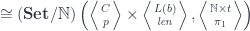
 is the projection from the cartesian product.
![(\mathbf{Set}/\mathbb{N})\left(\left \langle {C \atop p} \right \rangle, \left[ \left \langle {L(b) \atop \mathit{len}} \right \rangle, \left \langle {\mathbb{N} \times t \atop \pi_1} \right \rangle \right] \right)](https://s0.wp.com/latex.php?latex=%28%5Cmathbf%7BSet%7D%2F%5Cmathbb%7BN%7D%29%5Cleft%28%5Cleft+%5Clangle+%7BC+%5Catop+p%7D+%5Cright+%5Crangle%2C+%5Cleft%5B+%5Cleft+%5Clangle+%7BL%28b%29+%5Catop+%5Cmathit%7Blen%7D%7D+%5Cright+%5Crangle%2C+%5Cleft+%5Clangle+%7B%5Cmathbb%7BN%7D+%5Ctimes+t+%5Catop+%5Cpi_1%7D+%5Cright+%5Crangle+%5Cright%5D+%5Cright%29+&bg=ffffff&fg=29303b&s=0&c=20201002)
 and get:
![O(a, b; s, t) \cong \mathbf{Set} \left( s, U\left( \left[ \left \langle {L(b) \atop \mathit{len}} \right \rangle, \left \langle {\mathbb{N} \times t \atop \pi_1} \right \rangle \right] \times \left \langle {L(a) \atop \mathit{len}} \right \rangle \right) \right)](https://s0.wp.com/latex.php?latex=O%28a%2C+b%3B+s%2C+t%29+%5Ccong+%5Cmathbf%7BSet%7D+%5Cleft%28+s%2C+U%5Cleft%28+%5Cleft%5B+%5Cleft+%5Clangle+%7BL%28b%29+%5Catop+%5Cmathit%7Blen%7D%7D+%5Cright+%5Crangle%2C+%5Cleft+%5Clangle+%7B%5Cmathbb%7BN%7D+%5Ctimes+t+%5Catop+%5Cpi_1%7D+%5Cright+%5Crangle+%5Cright%5D+%5Ctimes+%5Cleft+%5Clangle+%7BL%28a%29+%5Catop+%5Cmathit%7Blen%7D%7D+%5Cright+%5Crangle+%5Cright%29+%5Cright%29+&bg=ffffff&fg=29303b&s=0&c=20201002)


 . The breakthrough came with the realization that, if


 defined by the unique property of leaving things alone
 , a long period of general stagnation accompanied by lack of change followed.
 , which ignores one of its inputs


 happens to have a similar decomposition
 . The Twinklean industry was based on the principle of mass production; and mass production starts with duplication and reuse. Suppose you have a reusable part


 .
.


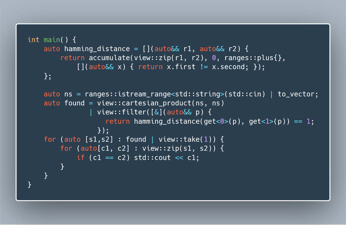

 is a shorthand for the hom-set
  .
. 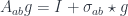
 is the (indexed) store comonad, which can be written as:
 is the constant functor, and
  is the hom-functor. In Haskell, this is equivalent to:
 (morphisms are functions
  that make the obvious triangles commute).
 the functor that generates a free applicative functor (or, equivalently, a free monoidal functor). Its fixed point can be written as:
 is a “list of”
 corresponds, in Haskell, to the existential data type we used in the definition of
  under the coend, the first step is to use the co-Yoneda lemma to “perform the integration” over
  , which replaces

 with
with  :
:
![Nat(h, g) \cong \int_{f \colon [C, Set]} Set(Nat(g, f), Nat(h, f))](https://s0.wp.com/latex.php?latex=Nat%28h%2C+g%29+%5Ccong+%5Cint_%7Bf+%5Ccolon+%5BC%2C+Set%5D%7D+Set%28Nat%28g%2C+f%29%2C+Nat%28h%2C+f%29%29&bg=ffffff&fg=29303b&s=0&c=20201002)
 is a set of higher-order natural transformations between them.
 and
and  to be either representable, or somehow related to representables.
 , and
, and ![[C, Set]](https://s0.wp.com/latex.php?latex=%5BC%2C+Set%5D&bg=ffffff&fg=29303b&s=0&c=20201002) :
:
 is the left adjoint to the forgetful functor
  :
:](https://s0.wp.com/latex.php?latex=App%28F+g%2C+f%29+%5Ccong+%5BC%2C+Set%5D%28g%2C+U+f%29&bg=ffffff&fg=29303b&s=0&c=20201002)
) \cong \int_{f \colon App} Set([C, Set](g, U f), [C, Set](h, U f))](https://s0.wp.com/latex.php?latex=%5BC%2C+Set%5D%28h%2C+U+%28F+g%29%29+%5Ccong+%5Cint_%7Bf+%5Ccolon+App%7D+Set%28%5BC%2C+Set%5D%28g%2C+U+f%29%2C+%5BC%2C+Set%5D%28h%2C+U+f%29%29&bg=ffffff&fg=29303b&s=0&c=20201002)


 , we can use the Yoneda lemma to “perform the integration” and arrive at:
 , this is exactly the free applicative generated by
  -valued functors, although a generalization to the enriched setting is relatively straightforward.
  and a unit
  :
: