In my previous post I worked on stretching the intuition of what a container is. I proposed that, in Haskell, any functor may be interpreted as some kind of container, including the hard cases like the state functor or the IO functor. I also talked about natural transformations between functors as “repackaging” schemes for containers, which work without “breaking the eggs” — not looking inside the elements stored in the container. Continuing with this analogy: Algebras are like recipes for making omelets.

The intuition is that an algebra provides a way to combine elements stored inside a container. This cannot be done for arbitrary types because there is no generic notion of “combining.” So an algebra is always defined for a specific type. For instance, you can define an algebra for numbers because you know how to add or multiply them, or for strings because you can concatenate them, and so on. The way elements are combined by an algebra is in general driven by the structure of the container itself.

For example, think of an expression tree as a container.

data Expr a = Const a 
            | Add (Expr a) (Expr a) 
            | Mul (Expr a) (Expr a)

We could define many algebras for it. An integer algebra would work on an expression tree that stores integers. A complex algebra would work on a tree that stores complex numbers. A Boolean algebra would work on Boolean expressions using, for instance, logical OR to evaluate the Add node and logical AND for the Mul node. You could even define an algebra of sets with union and intersection for Add and Mul. In fact, in the absence of any additional requirements, any pair of binary functions acting on a given type will do.

The definition of an algebra for a given functor f consists of a type t called the carrier type and a function called the action. Any Haskell algebra is therefore of the type:

newtype Algebra f t = Algebra (f t -> t)

More abstractly, in category theory, an algebra (or, more precisely, an F-algebra) for an endofunctor F is a pair (A, alg) of an object A and a morphism alg : F A -> A. As always, the standard translation from category theory to Haskell replaces objects with types and morphisms with functions.

Let’s have a look at a simple example of an algebra. Let’s pick the list functor and define an Int algebra for it, for instance:

sumAlg :: Algebra [] Int
sumAlg = Algebra (foldr (+) 0)

Despite its simplicity, this example leads to some interesting observations.

First, the use of foldr tells us that it’s possible to handle recursion separately from evaluation. The evaluation is really parameterized here by the function (+) and the value, zero. The algebra is type-specific. On the other hand, foldr is fully polymorphic. It turns out that there is another algebra hidden in this example, and it’s determined just by (+) and zero. We’ll see that more clearly when we talk about fixed points of functors.

The second observation is that a list is not only a functor but also a monad. Is there something special about algebras for a monad? We’ll see.

Algebras and Fixed Points

I wrote a whole blog post about F-algebras with a more categorical slant. Here I’ll elaborate on the Haskell aspects of algebras and develop some more intuitions.

A recursive container is not only a functor but it can also be defined as a fixed point of a functor. So, really, we should start with a double functor, parameterized by two types, a and b:

data ExprF a b = Const a
               | Add b b
               | Mul b b
     deriving Functor

We can then find its fixed point: a type that, when substituted for b, will give back itself. Think of a functor as a TV camera (sorry for switching metaphors). When you point it at some type b, its image appears in all the little monitors where b is on the right hand side of the definition. We all know what happens when you point the camera back at the monitors — you get the ever receding image within image within image… That’s your fixed point.

This “pointing of the camera at the monitors” can be abstracted into a Haskell data structure. It is parameterized by a functor f, which provides the camera and the monitors. The fixed point is given by the ever receding:

newtype Fix f = In (f (Fix f))

Notice that, on the left hand side, f appears without an argument. If f a is a container of a then f by itself is a recipe for creating a container from any type. Fix takes such a recipe and applies it to itself — to (Fix f).

Later we’ll also need the deconstructor, unIn:

unIn :: Fix f -> f (Fix f)
unIn (In x) = x

Going back to our earlier functor, we can apply Fix to it and get back the recursive version of Expr:

type Expr a = Fix (ExprF a)

Here, (ExprF a) is a recipe for stuffing any type b into a simple (non-recursive) container defined by ExprF.

Creating actual expressions using the above definition of Expr is a little awkward, but possible. Here’s one:

testExpr :: Expr Int
testExpr = In $ (In $ (In $ Const 2) `Add` (In $ Const 3)) 
                `Mul` (In $ Const 4)

Knowing that a recursive data type such as (Expr a) is defined in terms of a simpler functor (ExprF a b) means that any recursive algebra for it can be defined in terms of a simpler algebra. For instance, we can define a simple algebra for (ExprF Int) by picking the carrier type Double and the following action:

alg :: ExprF Int Double -> Double
alg (Const i) = fromIntegral i
alg (Add x y) = x + y
alg (Mul x y) = x * y

We can extend this algebra to work on arbitrary recursive expressions of type Expr Int. We’ll call this new recursive algebra alg'. When given an (Expr Int) it will do the following:

1. Extract the contents of the outer Fix by pattern matching on the consturctor In. The contents is of the type ExprF acting on (Expr Int).
2. Apply alg' (the recursive one we are just defininig) to this contents. Do this using fmap. Here we are taking advantage of the fact that ExprF is a functor. This application of alg' replaces the children of the expression ExprF with Doubles — the results of their evaluation.
3. Apply alg to the result of the previous step, which is of the type (ExprF Int Double).

Here’s the code that implements these steps:

alg' :: Fix (ExprF Int) -> Double
alg' (In expr) = alg (fmap alg' expr)

Notice that this code does not depend on the details of the functor. In fact it will work for any functor and any algebra:

cata :: Functor f => (f a -> a) -> Fix f -> a
cata alg = alg . fmap (cata alg) . unIn

This generic function is called a catamorphism. It lets you apply an algebra to the contents of a recursively defined container.

My first example of an algebra was acting on a list. A list can also be defined as a fixed point of a functor:

data ListF a b = Empty | Cons a b
     deriving Functor

If you work out the details, you can convince yourself that the sumAlg I defined earlier is nothing else but the catamorphism for the functor ListF Int applied to the following simple algebra:

alg :: ListF Int Int -> Int
alg Empty = 0
alg (Cons a b) = a + b

Now we understand why any list catamorphism is parameterized by one value and one function of two arguments.

Monads and Algebras

As I said in the beginning, a list is not only a functor but also a monad. A monad adds two special abilities to a functor/container. It lets you create a default container that contains just a given value: The function that does it is called return. And it lets you collapse a container of containers into a single container: That function is called join (and I explained before how it relates to the more commonly used bind, >>=).

When we define an algebra for a functor that happens to be a monad, it would be nice for this algebra to interact sensibly with return and join. For instance, you can apply return to a value of the algebra’s carrier type to obtain a default container of that type. Evaluating such a container should be trivial — it should give you back the same value:

(1) alg . return == id

For instance, in the list monad return creates a singleton list, so we want the algebra to extract the value from a singleton without modifying it in any way.

alg [a] =
(alg . return) a =
id a =
a

Now let’s consider a container of containers of the carrier type. We have two ways of collapsing it: we can fmap our algebra over it — in other words, evaluate all the sub-containers — or we can join it. Expecting to get the same result in both cases would be asking a lot (but we get something like this in the Kleisli category later). We can demand though that, for an algebra to be compatible with a monad, the two resulting containers at least evaluate to the same thing:

(2) alg . fmap alg == alg . join

Let’s see what this condition means for lists, where join is concatenation. We start with a list of lists and we apply two evaluation strategies to it: We can evaluate the sub-lists and then evaluate the resulting list of results, or we can concatenate the sub-lists and then evaluate the concatenated list.

Guess what, our condition is equivalent to imposing associativity on the algebra. Think of the action of the algebra on a two-element list as some kind of “multiplication.” Since the concatenation of [a, [b, c]] is the same as the concatenation of [[a, b], c], these two must evaluate to the same value. But that’s just associativity of our “multiplication.”

How much can we extend this analogy with multiplication? Can we actually produce a unit element? Of course: The action of the algebra on an empty list:

e = alg []

Let’s check it: Apply our compatibility conditions to the list [[a], []]. This is the left hand side:

(alg . fmap alg) [[a], []] = 
alg [alg [a], alg []] = 
alg [a, e]

And this is the right hand side:

(alg . join) [[a], []] = 
alg [a] = 
a

So, indeed, e is the right unit of our “multiplication.” You can do the same calculation for [[], [a]] to show that it’s also the left unit.

We have an associative operation equipped with a unit — that’s called a monoid. So any list algebra compatible with the list’s monadic structure defines a monoid.

T-Algebras

An F-algebra that’s compatible with a monad (conditions (1) and (2) above), both built on the same functor, is called a T-algebra. I guess that’s because mathematicians replace F with T when they talk about monads. There may be many T-algebras for a given monad and in fact they form a category of their own.

This is not saying much, because requirements for a category are pretty minimal. You have to define arrows: here it would be homomorphisms of T-algebras. A homomorphism of algebras maps one carrier into another in such a way as to preserve the action.

In Haskell, a homomorphism of algebras would just be a function h from one carrier type to another such that:

h    :: A -> B
alg  :: F A -> A
alg' :: F B -> B

h . alg == alg' . fmap h

Here, alg and alg' are the two actions with carrier types A and B, respectively, and F is the functor. What this means is that, if you have a container of As you can evaluate it using alg and then apply h to it and get a B, or you can apply h to the contents of the container using fmap and then evaluate the resulting container of Bs using alg'. The result should be the same in both cases.

This is a pretty standard way of defining homomorphisms for any structure, not just an algebra. Homomorphisms behave like functions: they are composable and there always is an identity homomorphism for every algebra, so they indeed turn T-algebras into a category — the so called Eilenberg-Moore category.

Remember what I said about the compatibility between join and alg? They both take down one layer of containment. Other than that, they are very different: join is a polymorphic natural transformation — it operates on the structure of the container, not its contents. An F-algebra operates on the contents and is defined only for a specific type.

And yet we can use join to define a T-algebra. Just consider using a container as a carrier type. A container is an image of some type a under a functor m which, for our purposes also happens to be a monad. Apply m to it one more time and you get a container of containers. You can “evaluate” this container of containers down to a single container using join.

You have just defined an algebra for the functor m whose carrier type is (m a) and the action is join. In fact, you have defined a whole family of algebras parameterized by the type a. Keep in mind that a is not the carrier type of this algebra, (m a) is. These algebras are called free algebras for the monad m. Guess what, they also form a category — the so called Kleisli category — which is a subcategory of the Eilenberg-Moore category.

Why are these two categories important? Well, it’s a topic for another blog post, but here’s the idea: Suppose you have two functors, F and G, one going from category C to D and the other going back. If G were the inverse of F, we would say that C and D are isomorphic. But what if they were “almost” inverse? For instance, their composition instead of being the identity were somehow mappable to identity. This kind of relationship between functors can be formalized into an adjunction. It so happens that the composition of two adjoint functors forms a monad (or a comonad, if you compose them the other way around). Not only that — any monad may be decomposed into a pair of adjoint functors. There are many ways to perform this decomposition and there are many choices for the intermediate category — the target of F and the source of G. The Kleisli category is the smallest such category and the Eilenberg-Moore category is the largest one.

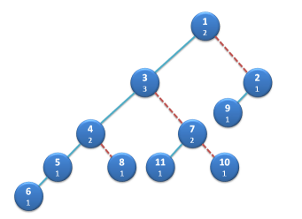
A heap is a great data structure for merging and sorting data. It’s implemented as a tree with the special heap property: A parent node is always less or equal than its children nodes, according to some comparison operator. In particular, the top element of the heap is always its smallest element. To guarantee quick retrieval and insertion, the tree doesn’t necessarily have to be well balanced. A leftist heap, for instance, is lopsided, with left branches always larger or equal to right branches.

The invariant of the leftist heap is expressed in terms of its right spines. The right spine of a tree is its rightmost path. Its length is called the rank of the tree. In a leftist heap the rank of the right child is always less or equal to the rank of the left child — the tree is leaning left. Because of that, the rank can grow at most logarithmically with the number of elements.

You can always merge two heaps by merging their right spines because they are just sorted linked lists. Since the right spines are at most logarithmically long, the merge can be done in logarithmic time. Moreover, it’s always possible to rotate nodes in the merged path to move heavier branches to the left and thus restore the leftist property.

With merging thus figured out, deletion from the top and insertion are trivial. After removing the top, you just merge left and right children. When inserting a new element, you create a singleton heap and merge it with the rest.

Implementation

The implementation of the functional leftist heap follows the same pattern we’ve seen before. We start with the definition:

A heap can either be empty or consist of a rank, a value, and two children: left and right heaps.

Let’s start with the definition of a non-empty heap as a private structure inside the Heap class:

template<class T>
class Heap
{
private:
    struct Tree
    {
        Tree(T v) : _rank(1), _v(v) {}
        Tree(int rank
            , T v
            , std::shared_ptr<const Tree> const & left
            , std::shared_ptr<const Tree> const & right)
        : _rank(rank), _v(v), _left(left), _right(right)
        {}

        int _rank;
        T   _v;
        std::shared_ptr<const Tree> _left;
        std::shared_ptr<const Tree> _right;
    };
    std::shared_ptr<Tree> _tree;
    ...
};

Heap data is just the shared_ptr<Tree>. An empty shared_ptr encodes an empty heap, otherwise it points to a non-empty Tree.

We’ll make the constructor of a non-empty heap private, because not all combinations of its arguments create a valid heap — see the two assertions:

Heap(T x, Heap const & a, Heap const & b)
{
    assert(a.isEmpty() || x <= a.front());
    assert(b.isEmpty() || x <= b.front());
    // rank is the length of the right spine
    if (a.rank() >= b.rank())
        _tree = std::make_shared<const Tree>(
                b.rank() + 1, x, a._tree, b._tree);
    else
        _tree = std::make_shared<const Tree>(
                a.rank() + 1, x, b._tree, a._tree);
}

We’ll make sure these assertions are true whenever we call this constructor from inside Heap code. This constructor guarantees that, as long as the two arguments are leftist heaps, the result is also a leftist heap. It also calculates the rank of the resulting heap by adding one to the rank of its right, shorter, branch. We’ll set the rank of an empty heap to zero (see implementation of rank).

As always with functional data structures, it’s important to point out that the construction takes constant time because the two subtrees are shared rather than copied. The sharing is thread-safe because, once constructed, the heaps are always immutable.

The clients of the heap will need an empty heap constructor:

Heap() {}

A singleton constructor might come in handy too:

explicit Heap(T x) : _tree(std::make_shared(x)) {}

They will need a few accessors as well:

bool isEmpty() const { return !_tree; }

int rank() const {
    if (isEmpty()) return 0;
    else return _tree->_rank;
}

The top, smallest, element is accessed using front:

T front() const { return _tree->_v; }

As I explained, the removal of the top element is implemented by merging left and right children:

Heap pop_front() const {
    return merge(left(), right()); 
}

Again, this is a functional data structure, so we don’t mutate the original heap, we just return the new heap with the top removed. Because of the sharing, this is a cheap operation.

The insertion is also done using merging. We merge the original heap with a singleton heap:

Heap insert(T x) {
    return merge(Heap(x), *this);
}

The workhorse of the heap is the recursive merge algorithm below:

static Heap merge(Heap const & h1, Heap const & h2)
{
    if (h1.isEmpty())
        return h2;
    if (h2.isEmpty())
        return h1;
    if (h1.front() <= h2.front())
        return Heap(h1.front(), h1.left(), merge(h1.right(), h2));
    else
        return Heap(h2.front(), h2.left(), merge(h1, h2.right()));
}

If neither heap is empty, we compare the top elements. We create a new heap with the smaller element at the top. Now we have to do something with the two children of the smaller element and the other heap. First we merge the right child with the other heap. This is the step I mentioned before: the merge follows the right spines of the heaps, guaranteeing logarithmic time. The left child is then combined with the result of the merge. Notice that the Heap constructor will automatically rotate the higher-rank tree to the left, thus keeping the leftist property. The code is surprisingly simple.

You might wonder how come we are not worried about the trees degenerating — turning into (left leaning) linked lists. Consider, however, that such a linked list, because of the heap property, would always be sorted. So the retrieval of the smallest element would still be very fast and require no restructuring. Insertion of an element smaller than the existing top would just prepend it to the list — a very cheap operation. Finally, the insertion of a larger element would turn this element into a length-one right spine — the right child of the top of the linked list. The degenerate case is actually our best case.

Turning an unsorted list of elements into a heap could naively be done in O(N*log(N)) time by inserting the elements one by one. But there is a better divide-and-conquer algorithm that does it in O(N) time (the proof that it’s O(N) is non-trivial though):

template<class Iter>
static Heap heapify(Iter b, Iter e)
{
    if (b == e)
        return Heap();
    if (e - b == 1)
        return Heap(*b);
    else
    {
        Iter mid = b + (e - b) / 2;
        return merge(heapify(b, mid), heapify(mid, e));
    }
}

This function is at the core of heap sort: you heapify a list and then extract elements from the top one by one. Since the extraction takes O(log(N)) time, you end up with a sort algorithm with the worst case performance O(N*log(N)). On average, heapsort is slower than quicksort, but quicksort’s worst case performance is O(N²), which might be a problem in some scenarios.

• Complete source code is available on GitHub.
• The previous blog post in this series was about functional data structures and concurrency.

For an outsider, Haskell is full of intimidating terms like functor, monad, applicative, monoid… These mathematical abstractions are hard to explain to a newcomer. The internet is full of tutorials that try to simplify them with limited success.

The most common simplification you hear is that a functor or a monad is like a box or a container. Indeed, a list is a container and a functor, Maybe is like a box, but what about functions? Functions from a fixed type to an arbitrary type define both a functor and a monad (the reader monad). More complex functions define the state and the continuation monads (all these monads are functors as well). I used to point these out as counterexamples to the simplistic picture of a functor as a container. Then I had an epiphany: These are containers!

So here’s the plan: I will first try to convince you that a functor is the purest expression of containment. I’ll follow with progressively more complex examples. Then I’ll show you what natural transformations really are and how simple the Yoneda lemma is in terms of containers. After functors, I’ll talk about container interpretation of pointed, applicative, and monad. I will end with a new twist on the state monad.

What’s a Container?

What is a container after all? We all have some intuitions about containers and containment but if you try to formalize them, you get bogged down with tricky cases. For instance, can a container be infinite? In Haskell you can easily define the list of all integers or all Pythagorean triples. In non-lazy language like C++ you can fake infinite containers by defining input iterators. Obviously, an infinite container doesn’t physically contain all the data: it generates it on demand, just like a function does. We can also memoize functions and tabulate their values. Is the hash table of the values of the sin function a container or a function?

The bottom line is that there isn’t that much of a difference between containers and functions.

What characterizes a container is its ability to contain values. In a strongly typed language, these values have types. The type of elements shouldn’t matter, so it’s natural to describe a generic container as a mapping of types — element type to container type. A truly polymorphic container should not impose any constraints on the type of values it contains, so it is a total function from types to types.

It would be nice to be able to generically describe a way to retrieve values stored in a container, but each container provides its own unique retrieval protocol. A retrieval mechanism needs a way to specify the location from which to retrieve the value and a protocol for failure. This is an orthogonal problem and, in Haskell, it is addressed by lenses.

It would also be nice to be able to iterate over, or enumerate the contents of a container, but that cannot be done generically either. You need at least to specify the order of traversal. Even the simplest list can be traversed forwards or backwards, not to mention pre-, in-, and post-order traversals of trees. This problem is addressed, for instance, by Haskell’s Traversable functors.

But I think there is a deeper reason why we wouldn’t want to restrict ourselves to enumerable containers, and it has to do with infinity. This might sound like a heresy, but I don’t see any reason why we should limit the semantics of a language to countable infinities. The fact that digital computers can’t represent infinities, even those of the countable kind, doesn’t stop us from defining types that have infinite membership (the usual Ints and Floats are finite, because of the binary representation, but there are, for instance, infinitely many lists of Ints). Being able to enumerate the elements of a container, or convert it to a (possibly infinite) list means that it is countable. There are some operations that require countability: witness the Foldable type class with its toList function and Traversable, which is a subclass of Foldable. But maybe there is a subset of functionality that does not require the contents of the container to be countable.

If we restrain ourselves from retrieving or enumerating the contents of a container, how do we know the contents even exists? Because we can operate on it! The most generic operation over the contents of a container is applying a function to it. And that’s what functors let us do.

Container as Functor

Here’s the translation of terms from category theory to Haskell.

A functor maps all objects in one category to objects in another category. In Haskell the objects are types, so a functor maps types into types (so, strictly speaking, it’s an endofunctor). You can look at it as a function on types, and this is reflected in the notation for the kind of the functor: * -> *. But normally, in a definition of a functor, you just see a polymorphic type constructor, which doesn’t really look like a function unless you squint really hard.

A categorical functor also maps morphisms to morphisms. In Haskell, morphisms correspond to functions, so a Functor type class defines a mapping of functions:

fmap :: (a -> b) -> (f a -> f b)

(Here, f is the functor in question acting on types a and b.)

Now let’s put on our container glasses and have another look at the functor. The type constructor defines a generic container type parameterized by the type of the element. The polymorphic function fmap, usually seen in its curried form:

fmap :: (a -> b) -> f a -> f b

defines the action of an arbitrary function (a -> b) on a container (f a) of elements of type a resulting in a container full of elements of type b.

Examples

Let’s have a look at a few important functors as containers.

There is the trivial but surprisingly useful container that can hold no elements. It’s called the Const functor (parameterized by an unrelated type b):

newtype Const b a = Const { getConst :: b }

instance Functor (Const b) where
    fmap _ (Const x) = Const x

Notice that fmap ignores its function argument because there isn’t any contents this function could act upon.

A container that can hold one and only one element is defined by the Identity functor:

newtype Identity a = Identity { runIdentity :: a }

instance Functor Identity where
    fmap f (Identity x) = Identity (f x)

Then there is the familiar Maybe container that can hold (maybe) one element and a bunch of regular containers like lists, trees, etc.

The really interesting container is defined by the function application functor, ((->) e) (which I would really like to write as (e-> )). The functor itself is parameterized by the type e — the type of the function argument. This is best seen when this functor is re-cast as a type constructor:

newtype Reader e a = Reader (e -> a)

This is of course the functor that underlies the Reader monad, where the first argument represents some kind of environment. It’s also the functor you’ll see in a moment in the Yoneda lemma.

Here’s the Functor instance for Reader:

instance Functor (Reader e) where  
    fmap f (Reader g) = Reader (\x -> f (g x))

or, equivalently, for the function application operator:

instance Functor ((->) e) where
    fmap = (.)

This is a strange kind of container where the values that are “stored” are keyed by values of type e, the environments. Given a particular environment, you can retrieve the corresponding value by simply calling the function:

runReader :: Reader e a -> e -> a
runReader (Reader f) env = f env

You can look at it as a generalization of the key/value store where the environment plays the role of the key.

The reader functor (for the lack of a better term) covers a large spectrum of containers depending of the type of the environment you pick. The simplest choice is the unit type (), which contains only one element, (). A function from unit is just a constant, so such a function provides a container for storing one value (just like the Identity functor). A function of Bool stores two values. A function of Integer is equivalent to an infinite list. If it weren’t for space and time limitations we could in principle memoize any function and turn it into a lookup table.

In type theory you might see the type of functions from A to B written as B^A, where A and B are types seen as sets. That’s because the analogy with exponentiation — taking B to the power of A — is very fruitful. When A is the unit type with just one element, B^A becomes B¹, which is just B: A function from unit is just a constant of type B. A function of Bool, which contains just two elements, is like B² or BxB: a Cartesian product of Bs, or the set of pairs of Bs. A function from the enumeration of N values is equivalent to an N-tuple of Bs, or an element of BxBxBx…B, N-fold. You can kind of see how this generalizes into B to the power of A, for arbitrary A.

So a function from A to B is like a huge tuple of Bs that is indexed by an element of A. Notice however that the values stored in this kind of container can only be enumerated (or traversed) if A itself is enumerable.

The IO functor that is the basis of the IO monad is even more interesting as a container because it offers no way of extracting its contents. An object of the type IO String, for instance, may contain all possible answers from a user to a prompt, but we can’t look at any of them in separation. All we can do is to process them in bulk. This is true even when IO is looked upon as a monad. All a monad lets you do is to pass your IO container to another monadic function that returns a new container. You’re just passing along containers without ever finding out if the Schrodinger’s cat trapped in them is dead or alive. Yes, parallels with quantum mechanics help a lot!

Natural Transformations

Now that we’ve got used to viewing functors as containers, let’s figure out what natural transformations are. A natural transformation is a mapping of functors that preserves their functorial nature. If functor F maps object A to X and another functor G maps A to Y, then a natural transformation from F to G must map X to Y. A mapping from X to Y is a morphism. So you can look at a natural transformation as a family of morphisms parameterized by A.

In Haskell, we turn all these objects A, X, and Y into types. We have two functors f and g acting on type a. A natural transformation will be a polymorphic function that maps f a to g a for any a.

forall a . f a -> g a

What does it mean in terms of containers? Very simple: A natural transformation is a way of re-packaging containers. It tells you how to take elements from one container and put them into another. It must do it without ever inspecting the elements themselves (it can, however, drop some elements or clone them).

Examples of natural transformations abound, but my favorite is safeHead. It takes the head element from a list container and repackages it into a Maybe container:

safeHead :: forall a . [a] -> Maybe a
safeHead []     = Nothing
safeHead (x:xs) = Just x

What about a more ambitions example: Let’s take a reader functor, Int -> a, and map it into the list functor [a]. The former corresponds to a container of a keyed by an integer, so it’s easily repackaged into a finite or an infinite list, for instance:

genInfList :: forall a . (Int -> a) -> [a]
genInfList f = fmap f [0..]

I’ll show you soon that all natural transformations from (Int -> a) to [a] have this form, and differ only by the choice of the list of integers (here, I arbitrarily picked [0..]).

A natural transformation, being a mapping of functors, must interact nicely with morphisms as well. The corresponding naturality condition translates easily into our container language. It tells you that it shouldn’t matter whether you first apply a function to the contents of a container (fmap over it) and then repackage it, or first repackage and then apply the function. This meshes very well with our intuition that repackaging doesn’t touch the elements of the container — it doesn’t breaks the eggs in the crate.

The Yoneda Lemma

Now let’s get back to the function application functor (the Reader functor). I said it had something to do with the Yoneda lemma. I wrote a whole blog about the Yoneda lemma, so I’m not going to repeat it here — just translate it into the container language.

What Yoneda says is that the reader is a universal container from which stuff can be repackaged into any other container. I just showed you how to repackage the Int reader into a list using fmap and a list of Int. It turns out that you can do the same for any type of reader and an arbitrary container type. You just provide a container full of “environments” and fmap the reader function over it. In my example, the environment type was Int and the container was a list.

Moreover, Yoneda says that there is a one-to-one correspondence between “repackaging schemes” and containers of environments. Given a container of environments you do the repackaging by fmapping the reader over it, as I did in the example. The inverse is also easy: given a repackaging, call it with an identity reader:

idReader :: Reader e e
idReader = Reader id

and you’ll get a container filled with environments.

Let me re-word it in terms of functors and natural transformations. For any functor f and any type e, all natural transformations of the form:

forall a . ((e -> a) -> f a)

are in one-to-one correspondence with values of the type f e. This is a pretty powerful equivalence. On the one hand you have a polymorphic function, on the other hand a polymorphic data structure, and they encode the same data. Except that things you do with functions are different than things you do with data structures so, depending on the context, one may be more convenient than the other.

For instance, if we apply the Yoneda lemma to the reader functor itself, we find out that all repackagings (natural transformations) between readers can be parameterized by functions between their environment types:

forall a . ((e -> a) -> (e' -> a)) ~ e' -> e

Or, you can look at this result as the CPS transform: Any function can be encoded in the Continuation Passing Style. The argument (e -> a) is the continuation. The forall quantifier tells us that the return type of the continuation is up to the caller. The caller might, for instance, decide to print the result, in which case they would call the function with the continuation that returns IO (). Or they might call it with id, which is itself polymorphic: a -> a.

Where Do Containers Come From?

A functor is a type constructor — it operates on types — but in a program you want to deal with data. A particular functor might define its data constructor: List and Maybe have constructors. A function, which we need in order to create an instance of the reader functor, may either be defined globally or through a lambda expression. You can’t construct an IO object, but there are some built-in runtime functions, like getChar or putChar that return IO.

If you have functions that produce containers you may compose them to create more complex containers, as in:

-- m is the functor
f :: a -> m b
g :: b -> m c
fmap g (f x) :: m (m c)

But the general ability to construct containers from scratch and to combine them requires special powers that are granted by successively more powerful classes of containers.

Pointed

The first special power is the ability to create a default container from an element of any type. The function that does that is called pure in the context of applicative and return in the context of a monad. To confuse things a bit more, there is a type class Pointed that defines just this ability, giving it yet another name, point:

class Functor f => Pointed f where
        point :: a -> f a

point is a natural transformation. You might object that there is no functor on the left hand side of the arrow, but just imagine seeing Identity there. Naturality just means that you can sneak a function under the functor using fmap:

fmap g (point x) = point (g x)

The presence of point means that there is a default, “trivial,” shape for the container in question. We usually don’t want this container to be empty (although it may — I’m grateful to Edward Kmett for correcting me on this point). It doesn’t mean that it’s a singleton, though — for ZipList, for instance, pure generates an infinite list of a.

Applicative

Once you have a container of one type, fmap lets you generate a container of another type. But since the function you pass to fmap takes only one argument, you can’t create more complex types that take more than one argument in their constructor. You can’t even create a container of (non-diagonal) pairs. For that you need a more general ability: to apply a multi-argument function to multiple containers at once.

Of course, you can curry a multi-argument function and fmap it over the first container, but the result will be a container of hungry functions waiting for more arguments.

h :: a -> b -> c
fmap h (m a) :: m (b -> c)

(Here, m stands for the functor, applicative, or the monad in question.)

What you need is the ability to apply a container of functions to a container of arguments. The function that does that is called <*> in the context of applicative, and ap in the context of monad.

(<*>) :: m (a -> b) -> m a -> m b

As I mentioned before, Applicative is also Pointed, with point renamed to pure. This lets you wrap any additional arguments to your multi-argument functions.

The intuition is that applicative brings to the table its ability to increase the complexity of objects stored in containers. A functor lets you modify the objects but it’s a one-input one-output transformation. An applicative can combine multiple sources of information. You will often see applicative used with data constructors (which are just functions) to create containers of object from containers of arguments. When the containers also carry state, as you’ll see when we talk about State, an applicative will also be able to reflect the state of the arguments in the state of the result.

Monad

The monad has the special power of collapsing containers. The function that does it is called join and it turns a container of containers into a single container:

join :: m (m a) -> m a

Although it’s not obvious at first sight, join is also a natural transformation. The fmap for the m . m functor is the square of the original fmap, so the naturality condition looks like this:

 fmap f . join = join . (fmap . fmap) f 

Every monad is also an applicative with return playing the role of pure and ap implementing <*>:

ap :: m (a -> b) -> m a -> m b
ap mf ma = join $ fmap (\f -> fmap f ma) mf

When working with the container interpretation, I find this view of a monad as an applicative functor with join more intuitive. In practice, however, it’s more convenient to define the monad in terms of bind, which combines application of a function a la fmap with the collapsing of the container. This is done using the function >>=:

(>>=) :: m a -> (a -> m b) -> m b
ma >>= k = join (fmap k ma)

Here, k is a function that produces containers. It is applied to a container of a, ma, using fmap. We’ve seen this before, but we had no way to collapse the resulting container of containers — join makes this possible.

Imagine a hierarchy of containment. You start with functions that produce containers. They “lift” your data to the level of containers. These are functions like putChar, data constructors like Just, etc. Then you have the “trivial” lifters of data called pure or return. You may operate on the data stored in containers by “lifting” a regular function using fmap. Applicative lets you lift multi-parameter functions to create containers of more complex data. You may also lift functions that produce containers to climb the rungs of containment: you get containers of containers, and so on. But only the monad provides the ability to collapse this hierarchy.

State

Let’s have a look at the state functor, the basis of the state monad. It’s very similar to the reader functor, except that it also modifies the environment. We’ll call this modifiable environment “state.” The modified state is paired with the return value of the function that defines the state functor:

newtype State s a = State (s -> (a, s))

As a container, the reader functor generalized the key/value store. How should we interpret the state functor in the container language? Part of it is still the key/value mapping, but we have the additional key/key mapping that describes the state transformation. (The state plays the role of the key.) Notice also that the action of fmap modifies the values, but doesn’t change the key mappings.

instance Functor (State s) where
  fmap f (State g) = State (\st -> let (x, st') = g st 
                                   in (f x, st'))

This is even more obvious if we separate the two mappings. Here’s the equivalent definition of the state functor in terms of two functions:

data State' s a = State' (s -> a) (s -> s)

The first function maps state to value: that’s our key/value store, identical to that of the reader functor. The second function is the state transition matrix. Their actions are quite independent:

runState' (State' f tr) s = (f s, tr s)

In this representation, you can clearly see that fmap only acts on the key/value part of the container, and its action on data is identical to that of the reader functor:

instance Functor (State' s) where
  fmap f (State' g tr) = State' (f . g) tr

In the container language, we like to separate the contents from the shape of the container. Clearly, in the case of the state functor, the transition matrix, not being influenced by fmap, is part of the shape.

A look at the Applicative instance for this representation of the state functor is also interesting:

instance Applicative (State' s) where
  pure x = State' (const x) id
  State' fg tr1 <*> State' fx tr2 =
      State' ff (tr2 . tr1)
    where
      ff st = let g = fg st
                  x = fx (tr1 st)
              in g x

The default container created by pure uses identity as its transition matrix. As expected, the action of <*> creates a new “shape” for the container, but it does it in a very regular way by composing the transition matrices. In the language of linear algebra, the transformation of state by the applicative functor would be called “linear.” This will not be true with monads.

You can also see the propagation of side effects: the values for the first and second argument are retrieved using different keys: The key for the retrieval of the function g is the original state, st; but the argument to the function, x, is retrieved using the state transformed by the transition matrix of the first argument (tr1 st). Notice however that the selection of keys is not influenced by the values stored in the containers.

But here’s the monad instance:

instance Monad (State' s) where
  return x = State' (const x) id
  State' fx tr >>= k =
      State' ff ttr
    where
      ff st  = let x = fx st
                   st' = tr st
                   State' fy tr' = k x
               in fy st' 
      ttr st = let x = fx st
                   st' = tr st
                   State' fy tr' = k x
               in tr' st'

What’s interesting here is that the calculation of the transition matrix requires the evaluation of the function k with the argument x. It means that the state transition is no longer linear — the decision which state to chose next may depend on the contents of the container. This is also visible in the implementation of join for this monad:

join :: State' s (State' s a) -> State' s a
join (State' ff ttr) = State' f' tr'
  where
    f' st  = let State' f tr = ff st
                 st'         = ttr st
             in f st'
    tr' st = let State' f tr = ff st
                 st'         = ttr st
             in tr st'

Here, the outer container stores the inner container as data. Part of the inner container is its transition matrix. So the decision of which transition matrix tr to use is intertwined with data in a non-linear way.

This non-linearity means that a monad is strictly more powerful than applicative, but it also makes composing monads together harder.

Conclusions

The only way to really understand a complex concept is to see it from as many different angles as possible. Looking at functors as containers provides a different perspective and brings new insights. For me it was the realization that functions can be seen as non-enumerable containers of values, and that the state monad can be seen as a key/value store with an accompanying state transition matrix that brought the aha! moments. It was also nice to explicitly see the linearity in the applicative’s propagation of state. It was surprising to discover the simplicity of the Yoneda lemma and natural transformations in the language of containers.

Bibliography and Acknowledgments

A container is not a very well defined term — an ambiguity I exploited in this blog post — but there is a well defined notion of finitary containers, and they indeed have a strong connection to functors. Russell O’Connor and Mauro Jaskelioff have recently shown that every traversable functor is a finitary container (I’m grateful to the authors for providing me with the preliminary copy of their paper, in which they have also independently and much more rigorously shown the connection between the Yoneda lemma for the functor category and the van Laarhoven formulation of the lens).