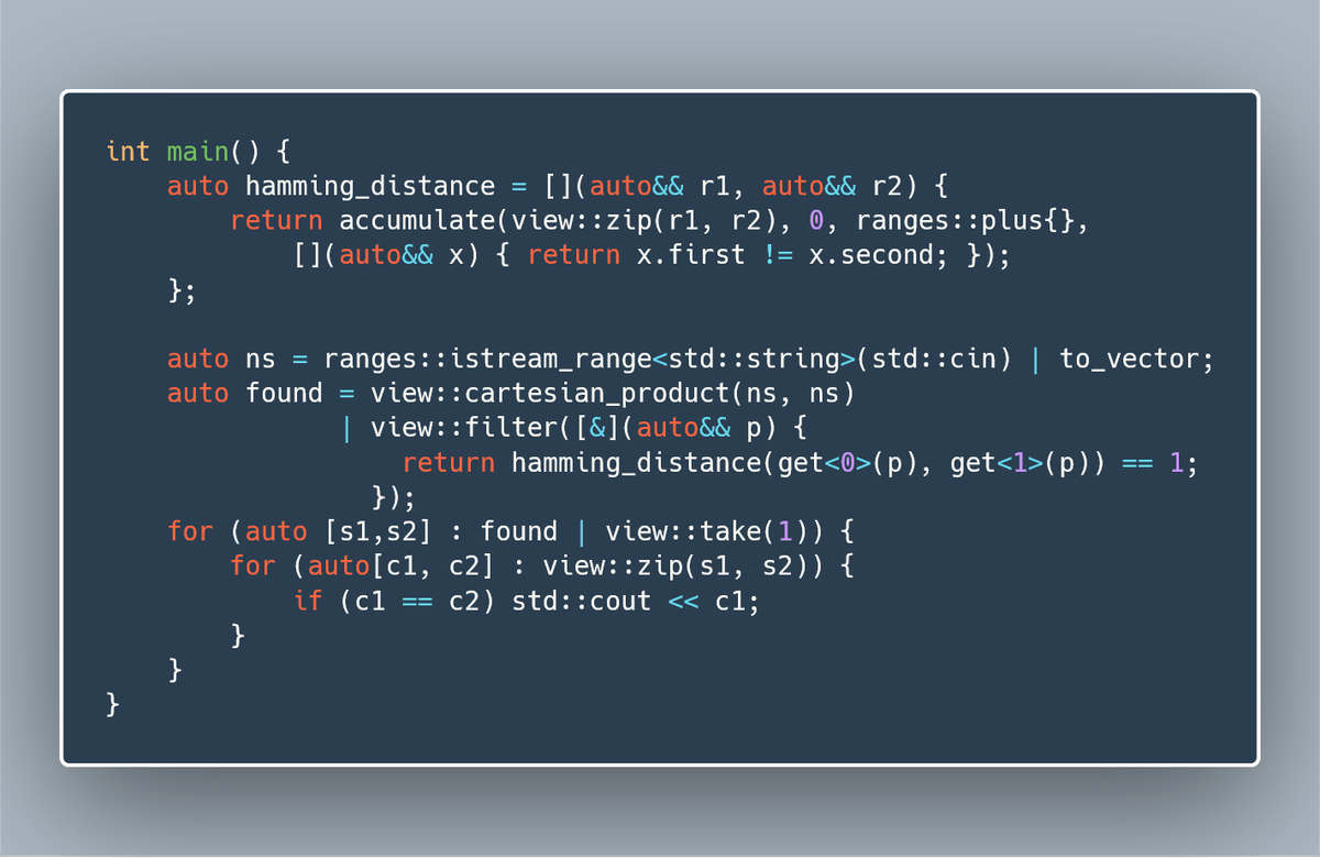
Yes, it’s this time of the year again! I started a little tradition a year ago with Stalking a Hylomorphism in the Wild. This year I was reminded of the Advent of Code by a tweet with this succint C++ program:

This piece of code is probably unreadable to a regular C++ programmer, but makes perfect sense to a Haskell programmer.
Here’s the description of the problem: You are given a list of equal-length strings. Every string is different, but two of these strings differ only by one character. Find these two strings and return their matching part. For instance, if the two strings were “abcd” and “abxd”, you would return “abd”.
What makes this problem particularly interesting is its potential application to a much more practical task of matching strands of DNA while looking for mutations. I decided to explore the problem a little beyond the brute force approach. And, of course, I had a hunch that I might encounter my favorite wild beast–the hylomorphism.
Brute force approach
First things first. Let’s do the boring stuff: read the file and split it into lines, which are the strings we are supposed to process. So here it is:
main = do
  txt <- readFile "day2.txt"
  let cs = lines txt
  print $ findMatch cs
The real work is done by the function findMatch, which takes a list of strings and produces the answer, which is a single string.
findMatch :: [String] -> String
First, let’s define a function that calculates the distance between any two strings.
distance :: (String, String) -> Int
We’ll define the distance as the count of mismatched characters.
Here’s the idea: We have to compare strings (which, let me remind you, are of equal length) character by character. Strings are lists of characters. The first step is to take two strings and zip them together, producing a list of pairs of characters. In fact we can combine the zipping with the next operation–in this case, comparison for inequality, (/=)–using the library function zipWith. However, zipWith is defined to act on two lists, and we will want it to act on a pair of lists–a subtle distinction, which can be easily overcome by applying uncurry:
uncurry :: (a -> b -> c) -> ((a, b) -> c)
which turns a function of two arguments into a function that takes a pair. Here’s how we use it:
uncurry (zipWith (/=))
The comparison operator (/=) produces a Boolean result, True or False. We want to count the number of differences, so we’ll covert True to one, and False to zero:
fromBool :: Num a => Bool -> a
fromBool False = 0
fromBool True  = 1
(Notice that such subtleties as the difference between Bool and Int are blisfully ignored in C++.)
Finally, we’ll sum all the ones using sum. Altogether we have:
distance = sum . fmap fromBool . uncurry (zipWith (/=))
Now that we know how to find the distance between any two strings, we’ll just apply it to all possible pairs of strings. To generate all pairs, we’ll use list comprehension:
let ps = [(s1, s2) | s1 <- ss, s2 <- ss]
(In C++ code, this was done by cartesian_product.)
Our goal is to find the pair whose distance is exactly one. To this end, we’ll apply the appropriate filter:
filter ((== 1) . distance) ps
For our purposes, we’ll assume that there is exactly one such pair (if there isn’t one, we are willing to let the program fail with a fatal exception).
(s, s') = head $ filter ((== 1) . distance) ps
The final step is to remove the mismatched character:
filter (uncurry (==)) $ zip s s'
We use our friend uncurry again, because the equality operator (==) expects two arguments, and we are calling it with a pair of arguments. The result of filtering is a list of identical pairs. We’ll fmap fst to pick the first components.
findMatch :: [String] -> String
findMatch ss =
  let ps = [(s1, s2) | s1 <- ss, s2 <- ss]
      (s, s') = head $ filter ((== 1) . distance) ps
  in fmap fst $ filter (uncurry (==)) $ zip s s'
This program produces the correct result and we could stop right here. But that wouldn’t be much fun, would it? Besides, it’s possible that other algorithms could perform better, or be more flexible when applied to a more general problem.
Data-driven approach
The main problem with our brute-force approach is that we are comparing everything with everything. As we increase the number of input strings, the number of comparisons grows like a factorial. There is a standard way of cutting down on the number of comparison: organizing the input into a neat data structure.
We are comparing strings, which are lists of characters, and list comparison is done recursively. Assume that you know that two strings share a prefix. Compare the next character. If it’s equal in both strings, recurse. If it’s not, we have a single character fault. The rest of the two strings must now match perfectly to be considered a solution. So the best data structure for this kind of algorithm should batch together strings with equal prefixes. Such a data structure is called a prefix tree, or a trie (pronounced try).
At every level of our prefix tree we’ll branch based on the current character (so the maximum branching factor is, in our case, 26). We’ll record the character, the count of strings that share the prefix that led us there, and the child trie storing all the suffixes.
data Trie = Trie [(Char, Int, Trie)]
  deriving (Show, Eq)
Here’s an example of a trie that stores just two strings, “abcd” and “abxd”. It branches after b.
   a 2
   b 2
c 1    x 1
d 1    d 1
When inserting a string into a trie, we recurse both on the characters of the string and the list of branches. When we find a branch with the matching character, we increment its count and insert the rest of the string into its child trie. If we run out of branches, we create a new one based on the current character, give it the count one, and the child trie with the rest of the string:
insertS :: Trie -> String -> Trie
insertS t "" = t
insertS (Trie bs) s = Trie (inS bs s)
  where
    inS ((x, n, t) : bs) (c : cs) =
      if c == x
      then (c, n + 1, insertS t cs) : bs
      else (x, n, t) : inS bs (c : cs)
    inS [] (c : cs) = [(c, 1, insertS (Trie []) cs)]
We convert our input to a trie by inserting all the strings into an (initially empty) trie:
mkTrie :: [String] -> Trie
mkTrie = foldl insertS (Trie [])
Of course, there are many optimizations we could use, if we were to run this algorithm on big data. For instance, we could compress the branches as is done in radix trees, or we could sort the branches alphabetically. I won’t do it here.
I won’t pretend that this implementation is simple and elegant. And it will get even worse before it gets better. The problem is that we are dealing explicitly with recursion in multiple dimensions. We recurse over the input string, the list of branches at each node, as well as the child trie. That’s a lot of recursion to keep track of–all at once.
Now brace yourself: We have to traverse the trie starting from the root. At every branch we check the prefix count: if it’s greater than one, we have more than one string going down, so we recurse into the child trie. But there is also another possibility: we can allow to have a mismatch at the current level. The current characters may be different but, since we allow only one mismatch, the rest of the strings have to match exactly. That’s what the function exact does. Notice that exact t is used inside foldMap, which is a version of fold that works on monoids–here, on strings.
match1 :: Trie -> [String]
match1 (Trie bs) = go bs
  where
    go :: [(Char, Int, Trie)] -> [String]
    go ((x, n, t) : bs) =
      let a1s = if n > 1
                then fmap (x:) $ match1 t
                else []
          a2s = foldMap (exact t) bs
          a3s = go bs -- recurse over list
      in a1s ++ a2s ++ a3s
    go [] = []
    exact t (_, _, t') = matchAll t t'
Here’s the function that finds all exact matches between two tries. It does it by generating all pairs of branches in which top characters match, and then recursing down.
matchAll :: Trie -> Trie -> [String]
matchAll (Trie bs) (Trie bs') = mAll bs bs'
  where
    mAll :: [(Char, Int, Trie)] -> [(Char, Int, Trie)] -> [String]
    mAll [] [] = [""]
    mAll bs bs' =
      let ps = [ (c, t, t')
               | (c,  _,  t)  <- bs
               , (c', _', t') <- bs'
               , c == c']
      in foldMap go ps
    go (c, t, t') = fmap (c:) (matchAll t t')
When mAll reaches the leaves of the trie, it returns a singleton list containing an empty string. Subsequent actions of fmap (c:) will prepend characters to this string.
Since we are expecting exactly one solution to the problem, we’ll extract it using head:
findMatch1 :: [String] -> String
findMatch1 cs = head $ match1 (mkTrie cs)
Recursion schemes
As you hone your functional programming skills, you realize that explicit recursion is to be avoided at all cost. There is a small number of recursive patterns that have been codified, and they can be used to solve the majority of recursion problems (for some categorical background, see F-Algebras). Recursion itself can be expressed in Haskell as a data structure: a fixed point of a functor:
newtype Fix f = In { out :: f (Fix f) }
In particular, our trie can be generated from the following functor:
data TrieF a = TrieF [(Char, a)]
  deriving (Show, Functor)
Notice how I have replaced the recursive call to the Trie type constructor with the free type variable a. The functor in question defines the structure of a single node, leaving holes marked by the occurrences of a for the recursion. When these holes are filled with full blown tries, as in the definition of the fixed point, we recover the complete trie.
I have also made one more simplification by getting rid of the Int in every node. This is because, in the recursion scheme I’m going to use, the folding of the trie proceeds bottom-up, rather than top-down, so the multiplicity information can be passed upwards.
The main advantage of recursion schemes is that they let us use simpler, non-recursive building blocks such as algebras and coalgebras. Let’s start with a simple coalgebra that lets us build a trie from a list of strings. A coalgebra is a fancy name for a particular type of function:
type Coalgebra f x = x -> f x
Think of x as a type for a seed from which one can grow a tree. A colagebra tells us how to use this seed to create a single node described by the functor f and populate it with (presumably smaller) seeds. We can then pass this coalgebra to a simple algorithm, which will recursively expand the seeds. This algorithm is called the anamorphism:
ana :: Functor f => Coalgebra f a -> a -> Fix f
ana coa = In . fmap (ana coa) . coa
Let’s see how we can apply it to the task of building a trie. The seed in our case is a list of strings (as per the definition of our problem, we’ll assume they are all equal length). We start by grouping these strings into bunches of strings that start with the same character. There is a library function called groupWith that does exactly that. We have to import the right library:
import GHC.Exts (groupWith)
This is the signature of the function:
groupWith :: Ord b => (a -> b) -> [a] -> [[a]]
It takes a function a -> b that converts each list element to a type that supports comparison (as per the typeclass Ord), and partitions the input into lists that compare equal under this particular ordering. In our case, we are going to extract the first character from a string using head and bunch together all strings that share that first character.
let sss = groupWith head ss
The tails of those strings will serve as seeds for the next tier of the trie. Eventually the strings will be shortened to nothing, triggering the end of recursion.
fromList :: Coalgebra TrieF [String]
fromList ss =
  -- are strings empty? (checking one is enough)
  if null (head ss)
  then TrieF [] -- leaf
  else
    let sss = groupWith head ss
    in TrieF $ fmap mkBranch sss
The function mkBranch takes a bunch of strings sharing the same first character and creates a branch seeded with the suffixes of those strings.
mkBranch :: [String] -> (Char, [String])
mkBranch sss =
  let c = head (head sss) -- they're all the same
  in (c, fmap tail sss)
Notice that we have completely avoided explicit recursion.
The next step is a little harder. We have to fold the trie. Again, all we have to define is a step that folds a single node whose children have already been folded. This step is defined by an algebra:
type Algebra f x = f x -> x
Just as the type x described the seed in a coalgebra, here it describes the accumulator–the result of the folding of a recursive data structure.
We pass this algebra to a special algorithm called a catamorphism that takes care of the recursion:
cata :: Functor f => Algebra f a -> Fix f -> a
cata alg = alg . fmap (cata alg) . out
Notice that the folding proceeds from the bottom up: the algebra assumes that all the children have already been folded.
The hardest part of designing an algebra is figuring out what information needs to be passed up in the accumulator. We obviously need to return the final result which, in our case, is the list of strings with one mismatched character. But when we are in the middle of a trie, we have to keep in mind that the mismatch may still happen above us. So we also need a list of strings that may serve as suffixes when the mismatch occurs. We have to keep them all, because they might be matched later with strings from other branches.
In other words, we need to be accumulating two lists of strings. The first list accumulates all suffixes for future matching, the second accumulates the results: strings with one mismatch (after the mismatch has been removed). We therefore should implement the following algebra:
Algebra TrieF ([String], [String])
To understand the implementation of this algebra, consider a single node in a trie. It’s a list of branches, or pairs, whose first component is the current character, and the second a pair of lists of strings–the result of folding a child trie. The first list contains all the suffixes gathered from lower levels of the trie. The second list contains partial results: strings that were matched modulo single-character defect.
As an example, suppose that you have a node with two branches:
[ ('a', (["bcd", "efg"], ["pq"]))
, ('x', (["bcd"],        []))]
First we prepend the current character to strings in both lists using the function prep with the following signature:
prep :: (Char, ([String], [String])) -> ([String], [String])
This way we convert each branch to a pair of lists.
[ (["abcd", "aefg"], ["apq"])
, (["xbcd"],         [])]
We then merge all the lists of suffixes and, separately, all the lists of partial results, across all branches. In the example above, we concatenate the lists in the two columns.
(["abcd", "aefg", "xbcd"], ["apq"])
Now we have to construct new partial results. To do this, we create another list of accumulated strings from all branches (this time without prefixing them):
ss = concat $ fmap (fst . snd) bs
In our case, this would be the list:
["bcd", "efg", "bcd"]
To detect duplicate strings, we’ll insert them into a multiset, which we’ll implement as a map. We need to import the appropriate library:
import qualified Data.Map as M
and define a multiset Counts as:
type Counts a = M.Map a Int
Every time we add a new item, we increment the count:
add :: Ord a => Counts a -> a -> Counts a
add cs c = M.insertWith (+) c 1 cs
To insert all strings from a list, we use a fold:
mset = foldl add M.empty ss
We are only interested in items that have multiplicity greater than one. We can filter them and extract their keys:
dups = M.keys $ M.filter (> 1) mset
Here’s the complete algebra:
accum :: Algebra TrieF ([String], [String])
accum (TrieF []) = ([""], [])
accum (TrieF bs) = -- b :: (Char, ([String], [String]))
    let -- prepend chars to string in both lists
        pss = unzip $ fmap prep bs
        (ss1, ss2) = both concat pss
        -- find duplicates
        ss = concat $ fmap (fst . snd) bs
        mset = foldl add M.empty ss
        dups = M.keys $ M.filter (> 1) mset
     in (ss1, dups ++ ss2)
  where
      prep :: (Char, ([String], [String])) -> ([String], [String])
      prep (c, pss) = both (fmap (c:)) pss
I used a handy helper function that applies a function to both components of a pair:
both :: (a -> b) -> (a, a) -> (b, b)
both f (x, y) = (f x, f y)
And now for the grand finale: Since we create the trie using an anamorphism only to immediately fold it using a catamorphism, why don’t we cut the middle person? Indeed, there is an algorithm called the hylomorphism that does just that. It takes the algebra, the coalgebra, and the seed, and returns the fully charged accumulator.
hylo :: Functor f => Algebra f a -> Coalgebra f b -> b -> a
hylo alg coa = alg . fmap (hylo alg coa) . coa
And this is how we extract and print the final result:
print $ head $ snd $ hylo accum fromList cs
Conclusion
The advantage of using the hylomorphism is that, because of Haskell’s laziness, the trie is never wholly constructed, and therefore doesn’t require large amounts of memory. At every step enough of the data structure is created as is needed for immediate computation; then it is promptly released. In fact, the definition of the data structure is only there to guide the steps of the algorithm. We use a data structure as a control structure. Since data structures are much easier to visualize and debug than control structures, it’s almost always advantageous to use them to drive computation.
In fact, you may notice that, in the very last step of the computation, our accumulator recreates the original list of strings (actually, because of laziness, they are never fully reconstructed, but that’s not the point). In reality, the characters in the strings are never copied–the whole algorithm is just a choreographed dance of internal pointers, or iterators. But that’s exactly what happens in the original C++ algorithm. We just use a higher level of abstraction to describe this dance.
I haven’t looked at the performance of various implementations. Feel free to test it and report the results. The code is available on github.
Acknowledgments
I’m grateful to the participants of the Seattle Haskell Users’ Group for many helpful comments during my presentation.


![[\mathbf{Opt}^{op}, Set] \cong \mathbf{Tamb}](https://s0.wp.com/latex.php?latex=%5B%5Cmathbf%7BOpt%7D%5E%7Bop%7D%2C+Set%5D+%5Ccong+%5Cmathbf%7BTamb%7D&bg=ffffff&fg=29303b&s=0&c=20201002)
![\hat F \in [\mathbf{Opt}^{op}, Set]](https://s0.wp.com/latex.php?latex=%5Chat+F+%5Cin+%5B%5Cmathbf%7BOpt%7D%5E%7Bop%7D%2C+Set%5D&bg=ffffff&fg=29303b&s=0&c=20201002)


 . We assume that this product is associative and unital– up to isomorphism. It means that there is an invertible associator:


![\triangleright \colon \mathbf M \to [C, C]](https://s0.wp.com/latex.php?latex=%5Ctriangleright+%5Ccolon+%5Cmathbf+M+%5Cto+%5BC%2C+C%5D&bg=ffffff&fg=29303b&s=0&c=20201002)
 to the tensor product
  and its unit

 as the monoidal category.)

 arrow, replacing it with its horizontal conjoint
  . In a profunctor equipment, this is just a representable profunctor
  .
.  .
. 
 . It states that any 2-cell
  of the shape below can be uniquely factorized through the counit
  :
:


 along a horizontal 1-cell


 and in
  .
.  . In Haskell, we can define them as two types:
 , the comma category
  consists of pairs
  . In other words, it’s a category of arrows from the image of
  to some fixed object
  . Morphisms in the comma category are arrows
  in
in  that make the corresponding triangles in
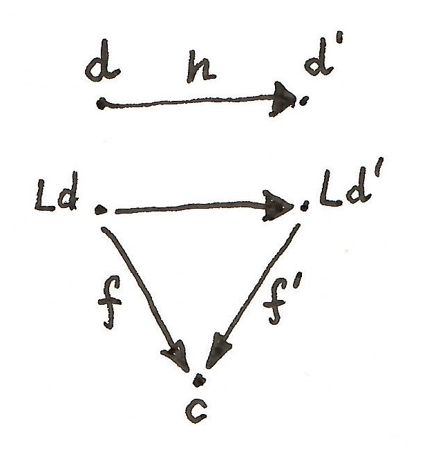
 , through which every arrow
  factorizes uniquely. That means, there is a unique arrow
  that makes the following triangle commute:
 , then we can easily construct the universal arrow as a pair
  , where
  is a component of the counit of the adjunction. Indeed, every
 .
.
 separately.
 , where
  is functor precomposition. Or as a string diagram:


 equipped with two natural transformations:


 also a comonad? Can we implement the two natural transformations for it?


 , again a comonad? We can easily define a counit:

 but it should be
  . To make it a comonad, we have to be able to push
  through
  in the middle. We need


 are in general not equal. All we can get from the original comonad laws is that they are only equal when applied to the result of comultiplication:
 .
. we can complete our definition of comultiplication for a composition of two comonads:

 ) and existential quantifiers (there exists,
  ).
).

 is written as
  . The resulting optic has two possible residues,


 in some monoidal category
  . There is an obvious forgetful functor
  that forgets the monoidal structure and produces an object of

 in which we identify some of the elements. Given a monoid homomorphism
  , and a pair of morphisms


 to extract monoidal values, transform these values to another monoid using
  , do the folding in the second monoid, and translate the result using
 to
to  and
and  , to a set
  . Being a functor, it also maps any pair of morphisms in


 .
.

 , between hom-sets:
 we have:
 to
to 
 . Their composition is another heteromorphism obtained by lifting the pair
  . Indeed:
 produces a heteromorphism from
  to
to  of a heteromorphism
  .
. and
and  are related this way if the hom-set
  , denoted by
  is defined as a path between objects. Objects
  and
and  are non-empty. As a witness of this relation we can pick any pair of elements, one from
  .
.

 equipped with a family of injections
 and a family:


 (we’ll switch to lower case to be compatible with Haskell) as
  . Einstein also came up with a clever convention: implicit summation over a repeated index. In the case of profunctors, the summation corresponds to taking a coend. In this notation, a coend over a profunctor


 and
and  behave like Kronecker deltas (in tensor-speak) or unit matrices. Here, the profunctor


 has categories as 0-cells, profunctors as 1-cells, and natural transformations as 2-cells. A natural transformation
  between profunctors

 and another,
  , having at our disposal two natural transformations:


 to
to 
 just happens to be a (strict) bicategory. It has (small) categories as 0-cells, functors as 1-cells, and natural transformations as 2-cells. A monad is defined as a combination of a 0-cell (you need a category to define a monad), an endo-1-cell (that would be an endofunctor in that category), and two 2-cells. These 2-cells are variably called multiplication and unit,
  and
and  , or
, or 

 is the hom-profunctor in the category


 for some
  . We’ll look for a function that would construct such an element in the following hom-set:
 .
. , as in the diagram below (courtesy Alex Campbell).