Bartosz Milewski's Programming Cafe

Previously we talked about dominant seventh chords, which are constructed by adding a minor seventh to a chord. Adding a major seventh instead is a very “jazzy” thing. With it, you can jazz up any chord, not just the dominant.

A major seventh is one semitone below the octave, so it forms a highly dissonant minor second (a single semitone) against it. This adds a lot of tension but, unlike the dominant seven, major dominant seventh doesn’t have an obvious resolution, so it provides an element of excitement and unpredictability.

Major-seventh chords are usually voiced in such a way as to put distance between the seventh and the root. But you can try this slightly unusual grip, in which there is a semitone interval between the two highest strings (although the third of the triad is missing, so it’s a variation of a power chord).

The notation for major-seventh chords varies–in jazz, the major seventh is often marked with a triangle, as in . It’s also common to see Maj in front of 7.

You may think of major-seventh chords as constructed either by lowering the root by a semitone, or raising the seventh of the corresponding dominant seventh chord.

Here’s the E major-seventh grip, together with its less common minor version:

When transposing these chords down the fretboard, we often skip the fifth in the bass as well as the root on the highest string. We either mute these strings or finger-pick the remaining four strings. Here’s the G major-seventh chord constructed this way:

You might be wondering at the resemblance of this grip to A minor. This is no coincidence–the major-seventh chord contains a minor triad. Check this out: there is a minor third between 3 and 5, and a major third between 5 and . In fact, every four-note chord contains two triads (the dominant seventh chord contained a diminished triad built inside a tritone, and the minor major-seventh chord contains an augmented triad).

Here are, similarly constructed, major-seventh versions of A chords. They are also easy to transpose down the fretboard. (Can you spot a flatted Dm shape in the first one?)

And these are the D chords:

C major-seventh is an odd one (that’s because there is an open string between the minor seventh and the root), but it’s very easy to grip:

If you squint hard enough, you can see the elements of E minor in it.

Here’s the open-string version of G major-seventh:

Squint again, and you can see the elements of B minor.

Next time: Adding the ninth.

Previously, we discussed chord construction by mutating the third (we’ll come back to the topic of mutating the fifth later). Another important mutation is adding more notes to a chord. Traditionally, the most common addition is that of the seventh. There are two versions of the seventh: minor, consisting of 10 semitones; and major, 11 semitones. We’ll start with the minor mutation, because it plays a very important role in functional harmony.

Classical music was built around the idea of tension and resolution, and the perfect expression of it was the authentic cadence, a two chord progression from the dominant chord to the tonic. The dominant is the fifth above the tonic so, for instance, E dominates A. You could build a whole song with just these two chords, and you’d probably end it on the cadence from E to A (the word cadence is derived from cadere, which means to fall).

To add more tension to a dominant chord, it is customary to extend it with a minor seventh. This creates a very dissonant interval between it and the third of the chord. The major third is 4 semitones above the root, the minor seventh is 10 semitones from the root, and 10 – 4 = 6. Six semitones is a diminished fifth, or the cursed tritone. The resolution of the tension created by this dissonance is very satisfying to our ears. A chord with a minor seventh is called the dominant seventh chord.

Let’s go back to the basic E shape and see how we can add a seventh to it.

We have two possibilities: we can either raise one of the fifth, or we can lower one of the roots. Luckily, both are duplicated, so we are not losing any triad tones.

Raising the fifth by three semitones (7 + 3 = 10) produces this grip:

Notice how smoothly it resolves down to the A chord by small movements of notes in opposite directions.

Here’s the alternative grip of E7, obtained by lowering the root (or the octave: 12 – 2 = 10) by two semitones:

This is a two-finger shape, and it’s easily transposed to any position on the fretboard. Alternatively, if you’re willing to skip the repeated fifth and the duplicated root, you may use this “jazzy” movable shape– here to voice a G7 at the third fret:

We can also add the minor seventh to minor chords to obtain minor seventh chords (sometimes called minor minor seventh chords). These are not as dissonant as their major counterparts (no tritone).

Again, we have two options, one of them easily movable across the fretboard

You can also mute the fifth in the second grip and obtain this strange chord:

This grip is often used in jazz, transposed across the fretboard, with either the top E string muted, or with both bass strings muted.

The story for the dominant seventh versions of the A chord is very similar:

And these are its two minor versions:

The D chords have only one dominant seven version each, obtained by lowering the root (octave):

And here’s the G7 chord in its usual shape, together with the truncated version which, incidentally, could be identified with the A7 chord shifted by two frets in the “wrong” direction:

We’ve seen the minor version of G seventh, Gm7, earlier.

There is only one version of C7:

Interestingly, it’s variation (the one with the fifth on the E string) can be shifted by one fret towards the nut to produce the B7 chord:

This new shape can, in turn, undergo further mutations, giving rise to other interesting extended chords.

As I said, dominant seventh chords have a strong tendency to resolve to their tonic chords, so it pays to learn at least part of the so called circle of fifths. Each chord in this list dominates the one to its right: B, E, A, D, G, C, F (followed by the sharped/flatted chords, to make the full circle of 12). The neighbor to the right of a given chord is called its subdominant. For instance E7 is the dominant of A, whose subdominant is D. The whole 12 bar blues can be played with any three consecutive chords picked from the circle of fifths.

Next time: major seventh chords.

So far we’ve been discussing chord transformations that didn’t change the chord’s function. We’ve been essentially dealing with just one major chord and its transpositions. You can think of a major chord as a rigid shape rotating through the circle of pitches: a four-semitone step topped with a three-semitone step, combining to seven semitones of the perfect fifth. We’ll keep the fifth for the time being, because it’s such a nice consonance, but we’ll be mutating the third.

The first such transformation is to lower the third by one semitone to obtain a minor triad. For some reason, we perceive minor chords as sad or melancholy, sometimes a bit whiny.

They are not very common in pop or rock music, but they are popular in folk and jazz (especially with added sevenths, which makes them edgy).

The first three shapes we’ve seen so far are perfect for this transformation: they have a single third, and it sits under a finger. Lifting or shifting this finger is easy. That changes the major third to a minor third, which we will notate as 3♭, since you can think of it as a flatted third. In jazz, flatting is often represented by a minus sign, so you might see Em notated as E-, and so on.

Here are the three basic minor shapes constructed this way:

When playing Dm, we usually mute the two lowest strings. I also listed the inversion Dm/F, as it’s sometimes used in chord progressions (e.g., a walking bass).

The C shape has the third voiced on an open string, and it’s doubled, so it’s humanly impossible to lower it. G shape is also tricky, although with the “folk” G you could cheat and mute the third, which results in a power chord. A power cord can be substituted, in a pinch, for either a major or a minor chord.

Normally, though, you produce all other minor chords by transposing (barring) either Em or Am.

It’s possible to move the third one more semitone step down or up. This results in suspended chords. Twice lowered third becomes a second, so that chord is called the suspended second. A raised third becomes a fourth, so that chord is called the suspended fourth. They are often used as embellishments, or in progression, with a regular major or minor chord in between (George Harrison’s Something or John Lennon’s Happy Xmas (War Is Over) use this riff extensively).

Suspended fourth works with the E shape as well

But suspended second in E is not very practical, since you have to use the adjacent string at the fourth fret, and you end up with the fifth in triplicate (of course, you can mute one).

Interestingly enough, the second can be reinterpreted as the ninth, an octave over. So, instead of using a suspended second, you may replace it with a better sounding add-nine chord. This one keeps the major third, but adds a ninth:

I’ll let you figure out suspensions for the C and G shapes.

Next: Dominant seventh chords.

Previously, we’ve seen how to transform the shapes of major chords by transposing them down the fretboard and across the fretboard. All these transformations can be composed. A mathematician would say that they form a group. Strictly speaking, one should introduce the identity transformation, which is just holding the same shape in place, and the inverse transformation. The latter is always possible, because the fretboard is cyclic: it repeats itself after the twelfth fret. So subtracting two frets is the same as adding ten frets.

Obviously, we can combine sideways shifts with vertical shifts and, for instance, produce the C chord by shifting down the A shape.

Even though all our shapes require only three fingers, the barred versions become progressively harder to grip as they require wider stretching of fingers. So the most common barred chords are either built from the E and A shapes, or use fewer than six strings (either by muting, or by finger picking).

And then there are some hybrid grips that merge multiple shapes. That’s because there is one more type of transformation, which I call “crawling,” where you move to a different triad note on the same string. We’ve already seen examples of creating variations of the G chord and the C chord by replacing the third by the fifth or vice versa. The third and the fifth are only separated by three frets, so they are often within easy reach. You have to be careful with replacing the third, though, if it wasn’t duplicated in the first place. For instance, here’s a version of the D chord that misses the third:

Such chords that only contain the root and the fifth are called power chords and are used a lot in heavy metal.

It’s also possible to replace the fifth by the root, as in this grip:

This is an interesting case of a hybrid grip. It started off as the A shape, but you may also see the beginnings of the G shape transposed down three frets, especially if you mute the two bass strings. The A shape has the ability to crawl down to a G shape.

Similarly, the D shape can crawl down to C shape (see the D triangle at the top?):

These two shapes (with the bass strings left out) can be easily transposed and are pretty useful in practice.

In fact, all chord shapes can be unified in one diagram, if you mark all triad tones across the fretboard. Here’s such a chart for the E chord. You can recognize, in order, the E shape, followed by the D shape, followed (and partially overlapped) by the C shape, which transitions into the A shape, which morphs into G, and finally goes back to E. You can use this diagram to play the same E chord in five different positions (after which it repeats itself).

You can, of course, produce such a chart starting from any of the five shapes, just by cycling it. Or you can cut this diagram out and glue it into a ring.

If you’re an astronomer, you might recognize some common constellations in this chart, like the Orion, or Draco, but that’s just pure coincidence.

Next time we’ll talk about minor chords.

Previously, we talked about transforming the basic E chord shape by transposing it up the fretboard. You may be aware that there are other chord shapes, sometimes grouped into the so called CAGED system. I’ll show you how to derive this system “scientifically.” Scientists arrive at new theories by looking at patterns. Sometimes a pattern doesn’t fit exactly, but it makes sense to temporarily ignore the discrepancy, forge ahead with incorrect assumptions, and then introduce subtle corrections to fix them. I know, this is not what they teach you in school, but that’s how it’s done in real life.

Let’s make some simplifying assumptions about guitar tuning. The first is that the top string can be identified with the bottom string: they are both E strings. Strictly speaking, this is not true: they are two octaves apart, and sometimes you can finger them differently, but we are playing scientists who ignore such distinctions. So we’ll consider the bottom E string a duplicate of the top E string. Second assumption is more outrageous: strings are tuned in fourths. Well, this is true in 80% of the cases. The 20% exception is the interval of a major third between the G string and the B string. We’ll just ignore it for the moment. With these assumptions in place, we can think of the strings forming a circle: we glue together the two E strings, and we get a circle of five strings a fourth apart.

In this imaginary world, we can now shift any chord shape sideways, around the circle, without changing its function. Granted, it will shift all the pitches up by a fourth, so shifting the E chord to the right would result in the A chord, another shift would produce the D chord, and so on. Lets try it!

We’ll start with the E chord and shift it to the right.

We get this:

Hurray! Within experimental error, it worked! Granted, this is the A minor chord, not the A major that we were expecting, but still, considering that our assumptions were partially wrong, that’s close enough.

The question is, how can we modify our theory to produce the A major chord? Our problem has its source in the anomaly between the G string and the B string. When we shift a finger between the two, keeping it on the same fret, we are not moving the pitch up by a fourth, we’re moving it by a third. If all shifts were by a fourth, relative intervals wouldn’t change, and we would just transpose a major chord into another major chord.

But not all is lost. It just means that we have to introduce a correction to our theory. In order to preserve relative intervals, when shifting from the G string to the B string, we have to move the finger one fret up the fretboard (or down, in the diagram). It works:

This is indeed the A major chord.

Of course, theory aside, the chord has to also sound right. This one is okay, except that the fifth of the triad is in the bass, which makes it an inverted chord. In guitar notation inversions are often written as slash chords; here it would be A/E, because of the E in the bass. Inverted chords don’t always work in a chord progressions so, in practice, people try to mute the low E and emphasize the root A.

To test our theory further, let’s apply the right shift to A. The fourth above A is D and, indeed we get the D major. Notice the adjustment when moving between the G and the B strings.

Again, the bass part is a little tricky. Here, I just duplicated the high E string grip on the lower E string, which resulted in another inversion D/F#. In practice, people usually mute both the E and the A strings and emphasize the root D.

Another shift to the right and we get the G chord (again, correcting the move from the G string to the B string and mirroring the E string):

This particular variant is often used in folk music. The more popular variant gets rid of the fifth on the B string, since the open B is the third of the triad.

This change leads to the duplication of the third, so people often mute the third in the bass.

Another shift, and we get the C major. Here, the move from the open G string is corrected by pressing the B string at the first fret. All according to our theory.

The third in the bass doesn’t sound good, so it’s usually muted. Another inversion, with the fifth in the bass, sounds better in many contexts, so here’s C/G:

Here’s another variant with, the fifth on the highest E string

We’ll see this variant modified by extension notes (the sevenths and the ninths).

We have just covered all the shapes in the CAGED system (the letters stand for the five major chords). And, indeed, we went full circle, because the next shift produces the F chord (the open G string turns into first fret press on the B string).

This makes perfect sense. If it weren’t for the anomaly, the fifth shift should bring us back to the same shape. But every time a black dot crosses the anomaly, it drops down so, after a full circle, the whole shape drops down one fret. Therefore five shifts to the right equal one shift down. We have just proven a theorem.

Notice that in the first three iterations a triangle shape is formed by three fingers. This shape consists of the fifth, the root, and the third of the triad. This information will come in handy when we discuss chord modifications. To the left of the triangle, we have the root, and to the right, another fifth (except in the D chord, where it’s pushed off the edge). In the G chord, we start seeing part of this triangle peeking on the left (the root and the third), shifted down because of the anomaly. In C/G the triangle is fully reconstituted, albeit one fret down. If you can spot these shapes, you’ll have no problem remembering where to find the third (and, for instance, lower it to make a minor chord) or where to insert the seventh.

This theory can be also visualized by arranging the strings in a radial pattern, the frets forming a spiral. Here’s the diagram for the E chord:

If you rotate the dots counterclockwise, you’ll get the A chord, and so on. The anomaly adjustment happens automatically, because the B string is offset by one step. Also, if no dot moves into the B string, a new dot at the first fret is produced.

Next time, combining the transformations.

We have our first guitar chord, E major:

We can apply a simple transformation to it to generate all of the major chords (there are twelve of them). The transformation is called transposition, and it simply moves all the notes up the fretboard by the same distance. We can easily move the three fingers that form the shape of E, but there are also three open strings. They have to be shifted as well. This is where barring with your index finger comes handy. Your finger creates a new nut (that’s what the upper end of the fretboard is called).

Below is the A major chord created by shifting E five semitones, or five frets, down the fretboard. The intervals don’t change, but the root changes from E to A, and all the notes get renamed accordingly.

This is how you grip it.

Technically, barring a chord, is not easy for beginners. You have to develop enough strength and precision in your left hand. But conceptually, it’s very simple. Shifting the whole shape doesn’t change relative intervals, so a major chord remains a major chord. If you don’t have perfect pitch, and somebody shifted a chord, you might not be able to tell. It’s all relative.

That’s why it reminds me of special relativity. You are looking at the same chord from a different frame of reference. All laws of physics (relative intervals) are the same. There is even an analog of relativistic shortening of distances (Lorenz contraction): the distances between frets get shorter as you move down the fretboard. If the frets continued all the way to the bridge, the distances between them would shrink to zero, and there would be infinitely many of them. Reaching the bridge is like reaching the speed of light in special relativity.

It’s very useful to know the names of frets on the E string, because each of them can become the root of a shifted chord. They are, starting from the zeroth fret, or the nut:

E, F, F#, G, G#, A, A#, B, C, C#, D, D#, E.

The twelveth fret is E again, one octave higher, and then the pattern repeats itself. As you can see, there is some regularity in the naming of notes, but then there are the odd cases. Every note can be sharped (the # sign) but you don’t see E# there because it’s the same as F. Also, B# is identified with C.

G major is barred on the third fret (three semitones from E):

and so on.

Later we’ll see that almost all chords with un-sharped names have alternative grips that don’t require barring. The odd one is F, which is really hard to play for beginners:

There is an alternative fingering that requires pressing two thinnest strings with the index finger and either not playing the thickest E string (muting it), or pressing it with a thumb wrapped around the stock:

Just for fun, here’s the F# major chord in which all the notes are sharped.

Perhaps surprisingly, transposition on the piano is much harder, because of the white key / black key irregularities.

Next time we’ll talk about the transformation that generates the CAGED system.

Music teaches us a lot about reality. It shows enough regularity to suggest a simple mathematical model, but also enough irregularity to frustrate our attempts at formalizing it. In this series of essays, I’ll try to describe some of this frustration mixed with fascination. I’m going to talk about the guitar; both because I know more about it and because it’s even more quirky than the piano.

The guitar is a versatile instrument. You can play individual notes of a melody, you can play chords, and you can play the bass line, sometimes all at the same time. All this with just six strings. These six strings are tuned is such a way as to maximize the number of chords that can be played on it. You play chords by making shapes with your left hand (or the right hand if, like Jimi Hendrix, you’re left-handed). It’s a very interesting optimization problem that involves equal parts of music theory and human anatomy.

Here are some anatomical constraints: we have five fingers in the string-pressing hand. The thumb is mostly used for grip, although you can sometimes use it to play bass notes on the thickest string by reaching around the neck. That leaves us with four fingers to control six strings. If we want to strum all six strings, we have two options: we can let two or more strings ring free, or use one of the fingers (usually the index finger) to bar multiple strings and use the remaining three fingers to create the chord shape. So the basic chord shape is a three-finger grip. If we can form a chord with three fingers, we can move it up the fretboard using the index finger for barring. As with all musical instruments, the available shapes are limited by anatomy: we can only stretch our fingers so much.

Now for some music theory. The basic chords are triads built from three notes: the root, the third, and the fifth (relative to the root). The intervals between these notes determine the type of the chord. A major triad is build from a major third and a minor third (the sum of these thirds is a perfect fifth–yes, in music 3 + 3 = 5). The C major triad, for instance, consists of three notes: C, E, and G. The distance from C to E is a major third, and the distance from E to G is a minor third. The distance from C to G is a perfect fifth.

Naively, we might think that the guitar should be tuned in thirds, say, the lowest string C, then E, and then G. But what then? What about the three remaining strings? We could repeat C, E, and G, an octave higher. That would be okay if we only wanted to play major triads. But there are also minor triads, with a minor third followed by a major third. C minor triad is C, E♭ (E flat), and G. So maybe we could use that for the tuning? It would allow us to play C minor with no fingers, and C major by pressing two strings with two fingers. Unfortunately, there are many other types of chords that would be very hard to play in that tuning, so this idea is scrapped.

Observe, though, that with six strings, it’s unavoidable that some notes of the triad would have to be doubled (modulo shifting by an octave or two). This introduces more intervals between notes: for instance, the distance from G to the C in the next octave is a fourth. So within a duplicated triad we have the intervals of a major third, minor third, the perfect fifth (their sum), a fourth (from G to C), as well as two sixths (from E to C and from G to E), a few octaves, and so on.

So here’s a new idea: If we tune the strings in fourths, we can easily, without stretching our fingers too much, produce thirds, fourths, and fifths. That’s because we can shorten an interval by pressing the lower sting, or lengthen it by pressing the higher string.

Let’s see how this works. The lowest string on the guitar is E, so that’s where we’ll start. A fourth about it is A, so that’s the next thickest string. Let’s see what intervals we can make using those two.

By pressing the E string at the first fret, we can produce a major third, F to A.

By pressing it at the second fret, we can produce a minor third, F# to A.

By releasing the E string and pressing the A string at the second fret, we can produce a perfect fifth, from E to B.

And, of course, by releasing both strings, we get a perfect fourth, from E to A. That’s a lot of handy intervals within easy reach.

Let’s use this idea to build the simplest guitar chord, E major, which contains E, G#, and B. In principle, the order of these notes and the octaves they are in doesn’t matter, but some combinations sound better than others. We’ll start with the open E string for the root. To start with, let’s assume the tuning in fourths, so the second string is A, the third D, and the fourth G.

We can can press the A string at the second fret to produce the fifth of the triad, B. (We are skipping G# for now, because it’s not easily reachable.)

The next triad note within reach is another E, an octave higher. We can play it by pressing the D string at the second fret.

Now we can finally add the third, G#, by pressing the next string, G, at the first fret.

We now have the root (doubled), the fifth, and the third of the triad.

There are two more strings to go, and we have already used three fingers to press three strings. If we continued tuning strings in fourths, the next string would be C. That’s not part of our triad, and we can’t easily stretch our pinky to reach the next E. So we begrudgingly give up on our rule of fourths, and instead tune the next string a semitone lower than we promised, to a B. B happens to be in our triad, so we’re fine. And a fourth about B is again E, so that works too.

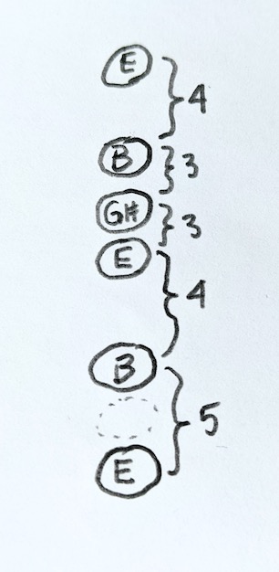
Here are the notes we used in this grip, together with intervals between them.

Notice that the root E is repeated three times, in different octaves. The fifth of the triad, B, appears twice, and the third, G#, only once. As we’ll see later, this arrangement gives us a lot of flexibility when transforming this grip.

The leap of a fifth in the bass, from E to B, is actually very pleasant to the ear — skipping the G# there is advantageous.

Here’s the same grip annotated with root-relative intervals. 1 is the root (E), 3 is the third (G#), and 5 is the fifth (B). It’s very important to remember which is which, in order to understand how to transform this shape to produce other interesting chords.

Not surprisingly, this is called the E shape in the popular CAGED system.

We’ve used only three fingers, which is great, because we’ll be able to use the index finger as a bar to move this triad up the fretboard, if we wish so.

In the process, we have arrived at the standard guitar tuning E, A, D, G, B, E. It is basically in fourth, except for the major third from G to B. This one exception introduces a lot of complexity into chord building on the guitar.

By now, you might have noticed some irregularities in music notation. They have accumulated over the centuries of development. We now use the so called equal temperament system in which the basic interval is a semitone, corresponding to one fret on the guitar. Standard musical intervals can be expressed in semitones, with the additional convenience that they satisfy standard arithmetic. For instance, a minor third is 3 semitones, a major third is 4 semitones, their sum is 7 semitones, corresponding to a perfect fifth. A perfect fourth is 5 semitones, which is an octave (12 semitones) minus the perfect fifth (7 semitones).

We could have motivated our tuning by postulating the distance of two octaves (24 semitones) between the lowest and the highest string. If we divide two octaves between six string (5 intervals), we get 4.8, which is almost the perfect fourth (5 semitones), but not quite. That’s why we introduced the “leap interval” of a major third between the G and the B strings.

Next, I’ll show you how all common chords and the majority of jazz chords can be derived from this single shape by applying various transformations (or, as mathematicians call them, morphisms).

Acknowledgment

I used the excellent free web program chordpic to generate my string diagrams.

The tremendous success, in recent centuries, of science and technology explaining the world around us and improving the human condition helped create the impression that we are on the brink of understanding the Universe. The world is complex, but we seem to have been able to reduce its complexity down to a relatively small number of fundamental laws. These laws are formulated in the language of mathematics, and the idea is that, even if we can’t solve all the equations describing complex systems, at least we can approximate the solutions, usually with the help of computers. These successes led to a feeling bordering on euphoria at the power of our reasoning. Eugene Wigner summed up this feeling in his famous essay, The Unreasonable Effectiveness of Mathematics in the Natural Sciences.

Granted, there are still a few missing pieces, like the unification of gravity with the Standard Model, and the 95% of the mass of the Universe unaccounted for, but we’re working on it… So there’s nothing to worry about, right?

Actually, if you think about it, the idea that the Universe can be reduced to a few basic principles is pretty preposterous. If this turned out to be the case, I would be the first to believe that we live in a simulation. It would mean that this enormous Universe, with all the galaxies, stars, and planets was designed with one purpose in mind: that a bunch of sentient monkeys on the third planet from a godforsaken star in a godforsaken galaxy were able to understand it. That they would be able to build, in their puny brains–maybe extended with some silicon chips and fiber optics–a perfect model of it.

How do we understand things? By building models in our (possibly computer-enhanced) minds. Obviously, it only makes sense if the model is smaller than the actual thing; which is only possible if reality is compressible. Now compare the size and the complexity of the Universe with the size and the complexity of our collective brains. Even with lossy compression, the discrepancy is staggering. But, you might say, we don’t need to model the totality of the Universe, just the small part around us. This is where compositionality becomes paramount. We assume that the world can be decomposed, and that the relevant part of it can be modeled, to a good approximation, independent from the rest.

Reductionism, which has been fueling science and technology, was made possible by the decompositionality of the world around us. And by “around us” I mean not only physical vicinity in space and time, but also proximity of scale. Consider that there are 35 orders of magnitude between us and the Planck length (which is where our most precious model of spacetime breaks down). It’s perfectly possible that the “sphere of decompositionality” we live in is but a thin membrane; more of an anomaly than a rule. The question is, why do we live in this sphere? Because that’s where life is! Call it anthropic or biotic principle.

The first rule of life is that there is a distinction between the living thing and the environment. That’s the primal decomposition.

It’s no wonder that one of the first “inventions” of life was the cell membrane. It decomposed space into the inside and the outside. But even more importantly, every living thing contains a model of its environment. Higher animals have brains to reason about the environment (where’s food? where’s predator?). But even a lowly virus encodes, in its DNA or RNA, the tricks it uses to break into a cell. Show me your RNA, and I’ll tell you how you spread. I’d argue that the definition of life is the ability to model the environment. And what makes the modeling possible is that the environment is decomposable and compressible.

We don’t think much of the possibility of life on the surface of a proton, mostly because we think that the proton is too small. But a proton is closer to our scale than it is to the Planck scale. A better argument is that the environment at the proton scale is not easily decomposable. A quarkling would not be able to produce a model of its world that would let it compete with other quarklings and start the evolution. A quarkling wouldn’t even be able to separate itself from its surroundings.

Once you accept the possibility that the Universe might not be decomposable, the next question is, why does it appear to be so overwhelmingly decomposable? Why do we believe so strongly that the models and theories that we construct in our brains reflect reality? In fact, for the longest time people would study the structure of the Universe using pure reason rather than experiment (some still do). Ancient Greek philosophers were masters of such introspection. This makes perfect sense if you consider that our brains reflect millions of years of evolution. Euclid didn’t have to build a Large Hadron Collider to study geometry. It was obvious to him that two parallel lines never intersect (it took us two thousand years to start questioning this assertion–still using pure reason).

You cannot talk about decomposition without mentioning atoms. Ancient Greeks came up with this idea by pure reasoning: if you keep cutting stuff, eventually you’ll get something that cannot be cut any more, the “uncuttable” or, in Greek, ἄτομον [atomon]. Of course, nowadays we not only know how to cut atoms but also protons and neutrons. You might say that we’ve been pretty successful in our decomposition program. But these successes came at the cost of constantly redefining the very concept of decomposition.

Intuitively, we have no problem imagining the Solar System as composed of the Sun and the planets. So when we figured out that atoms were not elementary, our first impulse was to see them as little planetary systems. That didn’t quite work, and we know now that, in order to describe the composition of the atom, we need quantum mechanics. Things are even stranger when decomposing protons into quarks. You can split an atom into free electrons and a nucleus, but you can’t split a proton into individual quarks. Quarks manifest themselves only under confinement, at high energies.

Also, the masses of the three constituent quarks add up only to one percent of the mass of the proton. So where does the rest of the mass come from? From virtual gluons and quark/antiquark pairs. So are those also the constituents of the proton? Well, sort of. This decomposition thing is getting really tricky once you get into quantum field theory.

Human babies don’t need to experiment with falling into a precipice in order to learn to avoid visual cliffs. We are born with some knowledge of spacial geometry, gravity, and (painful) properties of solid objects. We also learn to break things apart very early in life. So decomposition by breaking apart is very intuitive and the idea of a particle–the ultimate result of breaking apart–makes intuitive sense. There is another decomposition strategy: breaking things into waves. Again, it was Ancient Greeks, Pythagoras who studied music by decomposing it into harmonics, and Aristotle who suggested that sound propagates through movement of air. Eventually we uncovered wave phenomena in light, and then the rest of the electromagnetic spectrum. But our intuitions about particles and weaves are very different. In essence, particles are supposed to be localized and waves are distributed. The two decomposition strategies seem to be incompatible.

Enter quantum mechanics, which tells us that every elementary chunk of matter is both a wave and a particle. Even more shockingly, the distinction depends on the observer. When you don’t look at it, the electron behaves like a wave, the moment you glance at it, it becomes a particle. There is something deeply unsatisfying about this description and, if it weren’t for the amazing agreement with experiment, it would be considered absurd.

Let’s summarize what we’ve discussed so far. We assume that there is some reality (otherwise, there’s nothing to talk about), which can be, at least partially, approximated by decomposable models. We don’t want to identify reality with models, and we have no reason to assume that reality itself is decomposable. In our everyday experience, the models we work with fit reality almost perfectly. Outside everyday experience, especially at short distances, high energies, high velocities, and strong gravitational fields, our naive models break down. A physicist’s dream is to create the ultimate model that would explain everything. But any model is, by definition, decomposable. We don’t have a language to talk about non-decomposable things other than describing what they aren’t.

Let’s discuss a phenomenon that is borderline non-decomposable: two entangled particles. We have a quantum model that describes a single particle. A two-particle system should be some kind of composition of two single-particle systems. Things may be complicated when particles are close together, because of possible interaction between them, but if they move in opposite directions for long enough, the interaction should become negligible. This is what happens in classical mechanics, and also with isolated wave packets. When one experimenter measures the state of one of the particles, this should have no impact on the measurement done by another far-away scientist on the second particle. And yet it does! There is a correlation that Einstein called “the spooky action at a distance.” This is not a paradox, and it doesn’t contradict special relativity (you can’t pass information from one experimenter to the other). But if you try to stuff it into either particle or wave model, you can only explain it by assuming some kind of instant exchange of data between the two particles. That makes no sense!

We have an almost perfect model of quantum mechanical systems using wave functions until we introduce the observer. The observer is the Godzilla-like mythical beast that behaves according to classical physics. It performs experiments that result in the collapse of the wave function. The world undergoes an instantaneous transition: wave before, particle after. Of course an instantaneous change violates the principles of special relativity. To restore it, physicists came up with quantum field theory, in which the observers are essentially relegated to infinity (which, for all intents and purposes, starts a few centimeters away from the point of the violent collision in an collider). In any case, quantum theory is incomplete because it requires an external classical observer.

The idea that measurements may interfere with the system being measured makes perfect sense. In the macro world, when we shine the light on something, we don’t expect to disturb it too much; but we understand that the micro world is much more delicate. What’s happening in quantum mechanics is more fundamental, though. The experiment forces us to switch models. We have one perfectly decomposable model in terms of the Schroedinger equation. It lets us understand the propagation of the wave function from one point to another, from one moment to another. We stick to this model as long as possible, but a time comes when it no longer fits reality. We are forced to switch to a different, also decomposable, particle model. Reality doesn’t suddenly collapse. It’s our model that collapses because we insists–we have no choice!–on decomposability. But if nature is not decomposable, one model cannot possibly fit all of it.

What happens when we switch from one model to another? We have to initialize the new model with data extracted from the old model. But these models are incompatible. Something has to give. In quantum mechanics, we lose determinism. The transition doesn’t tell us how exactly to initialize the new model, it only gives us probabilities.

Notice that this approach doesn’t rely on the idea of a classical observer. What’s important is that somebody or something is trying to fit a decomposable model to reality, usually locally, although the case of entangled particles requires the reconciliation of two separate local models.

Model switching and model reconciliation also show up in the interpretation of the twin paradox in special relativity. In this case we have three models: the twin on Earth, the twin on the way to Proxima Centauri, and the twin on the way back. They start by reconciling their models–synchronizing the clocks. When the astronaut twin returns from the trip, they reconcile their models again. The interesting thing happens at Proxima Centauri, where the second twin turns around. We can actually describe the switch between the two models, one for the trip to, and another for the trip back, using more advanced general relativity, which can deal with accelerating frames. General relativity allows us to keep switching between local models, or inertial frames, in a continuous way. One could speculate that similar continuous switching between wave and particle models is what happens in quantum field theory.

In math, the closest match to this kind of model-switching is in the definition of topological manifolds and fiber bundles. A manifold is covered with maps–local models of the manifold in terms of simple n-dimensional spaces. Transitions between maps are well defined, but there is no guarantee that there exists one global map covering the whole manifold. To my knowledge, there is no theory in which such transitions would be probabilistic.

Seen from the distance, physics looks like a very patchy system, full of holes. Traditional wisdom has it that we should be able to eventually fill the holes and connect the patches. This optimism has its roots in the astounding series of successes in the first half of the twentieth century. Unfortunately, since then we have entered a stagnation era, despite record number of people and resources dedicated to basic research. It’s possible that it’s a temporary setback, but there is a definite possibility that we have simply reached the limits of decomposability. There is still a lot to explore within the decomposability sphere, and the amount of complexity that can be built on top of it is boundless. But there may be some areas that will forever be out of bounds to our reason.

Fig 1. Current decomposability sphere.

• GR: General Relativity (gravity)
• SR: Special Relativity
• PQFT: Perturbative Quantum Field Theory (compatible with SR)
• QM: Quantum Mechanics (non-relativistic)
• BB: Big Bang
• H: Higgs Field
• SB: Symmetry Breaking (inflation)