Previously, we talked about the construction of initial algebras. The dual construction is that of terminal coalgebras. Just like an algebra can be used to fold a recursive data structure into a single value, a coalgebra can do the reverse: it lets us build a recursive data structure from a single seed.

Here’s a simple example. We define a tree that stores values in its nodes

data Tree a = Leaf | Node a (Tree a) (Tree a)

We can build such a tree from a single list as our seed. We can choose the algorithm in such a way that the tree is ordered in a particular way

split :: Ord a => [a] -> Tree a
split [] = Leaf
split (a : as) = Node a (split l) (split r)
  where (l, r) = partition (<a) as

A traversal of this tree will produce a sorted list. We’ll get back to this example after working out some theory behind it.

The functor

The tree in our example can be derived from the functor

data TreeF a x = LeafF | NodeF a x x

instance Functor (TreeF a) where
  fmap _ LeafF = LeafF
  fmap f (NodeF a x y) = NodeF a (f x) (f y)

Let’s simplify the problem and forget about the payload of the tree. We’re interested in the functor

data F x = LeafF | NodeF x x

Remember that, in the construction of the initial algebra, we were applying consecutive powers of the functor to the initial object. The dual construction of the terminal coalgebra involves applying powers of the functor to the terminal object: the unit type () in Haskell, or the singleton set in .

Let’s build a few such trees. Here are a some terms generated by the single power of F

w1, u1 :: F ()
w1 = LeafF
u1 = NodeF () ()

And here are some generated by the square of F acting on ()

w2, u2, t2, s2 :: F (F ())

w2 = LeafF
u2 = NodeF w1 w1
t2 = NodeF w1 u1
s2 = NodeF u1 u1

Or, graphically

Notice that we are getting two kinds of trees, ones that have units () in their leaves and ones that don’t. Units may appear only at the -st layer (root being the first layer) of .

We are also getting some duplication between different powers of . For instance, we get a single LeafF at the level and another one at the level (in fact, at every consecutive level after that as well). The node with two LeafF leaves appears at every level starting with , and so on. The trees without unit leaves are the ones we are familiar with—they are the finite trees. The ones with unit leaves are new and, as we will see, they will contribute infinite trees to the terminal coalgebra . We’ll construct the terminal coalgebra as a limit of an -chain.

Terminal coalgebra as a limit

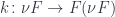
As was the case with initial algebras, we’ll construct a chain of powers of , except that we’ll start with the terminal rather than the initial object, and we’ll use a different morphism to link them together. By definition, there is only one morphism from any object to the terminal object. In category theory, we’ll call this morphism (upside-down exclamation mark) and implement it in Haskell as a polymorphic function

unit :: a -> ()
unit _ = ()

First, we’ll use to connect to , then lift to connect to , and so on, using to transform to .

Let’s see how it works in Haskell. Applying unit directly to F () turns it into ().

Values of the type F (F ()) are mapped to values of the type F ()

w2' = fmap unit w2
> LeafF
u2' = fmap unit u2
> NodeF () ()
t2' = fmap unit t2
> NodeF () ()
s2' = fmap unit s2
> NodeF () ()

and so on.

The following pattern emerges. contains trees that end with either leaves (at any level) or values of the unit type (only at the lowest, -st level). The lifted morphism (the st power of fmap acting on unit) operates strictly on the th level of a tree. It turns leaves and two-unit-nodes into single units ().

Alternatively, we can look at the preimages of these mappings—conceptually reversing the arrows. Observe that all trees at the level can be seen as generated from the trees at the level by replacing every unit () with either a leaf LeafF or a node NodeF ()().

It’s as if a unit were a universal seed that can either sprout a leaf or a two-unit-node. We’ll see later that this process of growing recursive data structures from seeds corresponds to anamorphisms. Here, the terminal object plays the role of a universal seed that may give rise to two parallel universes. These correspond to the inverse image (a so-called fiber) of the lifted unit.

Now that we have an -chain, we can define its limit. It’s easier to understand a limit in the category of sets. A limit in is a set of cones whose apex is the singleton set.

The simplest example of a limit is a product of sets. In that case, a cone with a singleton at the apex corresponds to a selection of elements, one per set. This agrees with our understanding of a product as a set of tuples.

A limit of a directed finite chain is just the starting set of the chain (the rightmost object in our pictures). This is because all projections, except for the rightmost one, are determined by commuting triangles. In the example below, is determined by :

and so on. Here, every cone from is fully determined by a function , and the set of such functions is isomorphic to .

Things are more interesting when the chain is infinite, and there is no rightmost object—as is the case of our -chain. It turns out that the limit of such a chain is the terminal coalgebra for the functor .

In this case, the interpretation where we look at preimages of the morphisms in the chain is very helpful. We can view a particular power of acting on as a set of trees generated by expanding the universal seeds embedded in the trees from the lower power of . Those trees that had no seeds, only LeafF leaves, are just propagated without change. So the limit will definitely contain all these trees. But it will also contain infinite trees. These correspond to cones that select ever growing trees in which there are always some seeds that are replaced with double-seed-nodes rather than LeafF leaves.

Compare this with the initial algebra construction which only generated finite trees. The terminal coalgebra for the functor TreeF is larger than the initial algebra for the same functor.

We have also seen a functor whose initial algebra was an empty set

data StreamF a x = ConsF a x

This functor has a well-defined non-empty terminal coalgebra. The -th power of (StreamF a) acting on () consists of lists of as

ConsF a1 (ConsF a2 (... (ConsF an ())...))

The lifting of unit acting on such a list replaces the final (ConsF a ()) with () thus shortening the list by one item. Its “inverse” replaces the seed () with any value of type a (so it’s a multi-valued inverse, since there are, in general, many values of a). The limit is isomorphic to an infinite stream of a. In Haskell it can be written as a recursive data structure

data Stream a = ConsF a (Stream a)

Anamorphism

The limit of a diagram is defined as a universal cone. In our case this would be the cone consisting of the object we’ll call , with a set of projections

such that any other cone factors through . We want to show that (if it exists) is a terminal coalgebra.

First, we have to show that is indeed a coalgebra, that is, there exists a morphism

We can apply to the whole diagram. If preserves -limits, then we get a universal cone with the apex and the -chain with on the left. But our original object forms a cone over the same chain (ignoring the projection ). Therefore there must be a unique mapping from it to .

The coalgebra is terminal if there is a unique morphism from any other coalgebra to it. Consider, for instance, a coalgebra . With this coalgebra, we can construct an -chain

We can connect the two omega chains using the terminal morphism from to and all its liftings

Notice that all squares in this diagram commute. The leftmost one commutes because is the terminal object, therefore the mapping from to it is unique, so the composite must be the same as . is therefore an apex of a cone over our original -chain. By universality, there must be a unique morphism from to the limit of this -chain, . This morphism is in fact a coalgebra morphism and is called the anamorphism.

Adjunction

The constructions of initial algebras and terminal coalgebras can be compactly described using adjunctions.

There is an obvious forgetful functor from the category of -algebras to . This functor just picks the carrier and forgets the structure map. Under certain conditions, the left adjoint free functor exists

This adjunction can be evaluated at the initial object (the empty set in ).

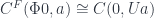
This shows that there is a unique algebra morphism—the catamorphism— from to any algebra . This is because the hom-set is a singleton for every . Therefore is the initial algebra .

Conversely, there is a cofree functor

It can be evaluated at a terminal object

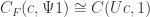
showing that there is a unique coalgebra morphism—the anamorphism—from any coalgebra to . This shows that is the terminal coalgebra .

Fixed point

Lambek’s lemma works for both, initial algebras and terminal coalgebras. It states that their structure maps are isomorphisms, therefore their carriers are fixed points of the functor

The difference is that is the least fixed point, and is the greatest fixed point of . They are, in principle, different. And yet, in a programming language like Haskell, we only have one recursively defined data structure defining the fixed point

newtype Fix f = Fix { unFix :: f (Fix f) }

So which one is it?

We can define both the catamorphisms from-, and anamorphisms to-, the fixed point:

type Algebra f a = f a -> a

cata :: Functor f => Algebra f a -> Fix f -> a
cata alg = alg . fmap (cata alg) . unfix

type Coalgebra f a = a -> f a

ana :: Functor f => Coalgebra f a -> a -> Fix f
ana coa = Fix . fmap (ana coa) . coa

so it seems like Fix f is both initial as the carrier of an algebra and terminal as the carrier of a coalgebra. But we know that there are elements of that are not in —namely infinite trees and infinite streams—so the two fixed points are not isomorphic and cannot be both described by the same Fix f.

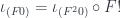
However, they are not unrelated. Because of the Lambek’s lemma, the initial algebra gives rise to a coalgebra , and the terminal coalgebra generates an algebra .

Because of universality, there must be a (unique) algebra morphism from the initial algebra to , and a unique coalgebra morphism from to the terminal coalgebra . It turns out that these two are given by the same morphism between the carriers. This morphism satisfies the equation

which makes it both an algebra and a coalgebra morphism

Furthermore, it can be shown that, in , is injective: it embeds in . This corresponds to our observation that contains plus some infinite data structures.

The question is, can Fix f describe infinite data? The answer depends on the nature of the programming language: infinite data structures can only exist in a lazy language. Since Haskell is lazy, Fix f corresponds to the greatest fixed point. The least fixed point forms a subset of Fix f (in fact, one can define a metric in which it’s a dense subset).

This is particularly obvious in the case of a functor that has no terminating leaves, like the stream functor.

data StreamF a x = StreamF a x
  deriving Functor

We’ve seen before that the initial algebra for StreamF a is empty, essentially because its action on Void is uninhabited. It does, however have a terminal coalgebra. And, in Haskell, the fixed point of the stream functor indeed generates infinite streams

type Stream a = Fix (StreamF a)

How do we know that? Because we can construct an infinite stream using an anamorphism. Notice that, unlike in the case of a catamorphism, the recursion in an anamorphism doesn’t have to be well founded and, indeed, in the case of a stream, it never terminates. This is why this won’t work in an eager language. But it works in Haskell. Here’s a coalgebra whose carrier is Int

coaInt :: Coalgebra (StreamF Int) Int
coaInt n = StreamF n (n + 1)

It generates an infinite stream of natural numbers

ints = ana coaInt 0

Of course, in Haskell, the work is not done until we demand some values. Here’s the function that extracts the head of the stream:

hd :: Stream a -> a
hd (Fix (StreamF x _)) = x

And here’s one that advances the stream

tl :: Stream a -> Stream a
tl (Fix (StreamF _ s)) = s

This is all true in , but Haskell is not . I had a discussion with Edward Kmett and he pointed out that Haskell’s fixed point data type can be considered the initial algebra as well. Suppose that you have an infinite data structure, like the stream we were just discussing. If you apply a catamorphism for an arbitrary algebra to it, it will most likely never terminate (try summing up an infinite stream of integers). In Haskell, however, this is interpreted as the catamorphism returning the bottom , which is a perfectly legitimate value. And once you start including bottoms in your reasoning, all bets are off. In particular Void is no longer uninhabited—it contains —and the colimit construction of the initial algebra is no longer valid. It’s possible that some of these results can be generalized using domain theory and enriched categories, but I’m not aware of any such work.

Bibliography

1. Adamek, Introduction to coalgebra
2. Michael Barr, Terminal coalgebras for endofunctors on sets

There is a bit of folklore about algebras in Haskell, which says that both the initial algebra and the terminal coalgebra for a given functor are defined by the same fixed point formula. This works for most common cases, but is not true in general. What is definitely true is that they are both fixed points–this result is called the Lambek’s lemma–but there may be many fixed points. The initial algebra is the least fixed point, and the terminal coalgebra is the greatest fixed point.

In this series of blog posts I will explore the ways one can construct these (co-)algebras using category theory and illustrate it with Haskell examples.

In this first installment, I’ll go over the construction of the initial algebra.

A functor

Let’s start with a simple functor that generates binary trees. Normally, we would store some additional data in a tree (meaning, the functor would take another argument), either in nodes or in leaves, but here we’re just interested in pure shapes.

data F a = Leaf 
         | Node a a
  deriving Show

Categorically, this functor can be written as a coproduct (sum) of the terminal object (singleton) and the product of with itself, here written simply as

The lifting of functions is given by this implementation of fmap

instance Functor F where
  fmap _ Leaf       = Leaf
  fmap f (Node x y) = Node (f x) (f y)

We can use this functor to build arbitrary level trees. Let’s consider, for instance, terms of type F Int. We can either build a Leaf, or a Node with two numbers in it

x1, y1 :: F Int
x1 = Leaf
y1 = Node 1 2 

With those, we can build next-level values of the type or, in our case, F (F Int)

x2, y2 :: F (F Int)
x2 = Leaf
y2 = Node x1 y1

We can display y2 directly using show

> Node Leaf (Node 1 2)

or draw the corresponding tree

Since is an endofunctor, so is . Lifting a function to can be implemented by applying fmap twice. Here’s the action of the function (+1) on our test values

fmap (fmap (+1)) x2
> Leaf
fmap (fmap (+1)) y2
> Node Leaf (Node 2 3)

or, graphically,

You can see that Leafs at any level remain untouched; only the contents of bottom Nodes in the tree are transformed.

The colimit construction

The carrier of the initial algebra can be constructed as a colimit of an infinite sequence. This sequence is constructed by applying powers of to the initial object which we’ll denote as . We’ll first see how this works in our example.

The initial object in Haskell is defined as a type with no data constructor (we are ignoring the question of non-termination in Haskell).

data Void
  deriving Show

In Set, this is just an empty set.

The Show instance for Void requires the pragma

{-# language EmptyDataDeriving #-}

Even though there are no values of the type Void, we can still construct a value of the type F Void

z1 :: F Void
z1 = Leaf

This degenerate version of a tree can be drawn as

This illustrates a very important property of our : Its action on an empty set does not produce an empty set. This is what allows us to generate a non-trivial sequence of powers of starting with the empty set.

Not every functor has this property. For instance, the construction of the initial algebra for the functor

data StreamF a x = ConsF a x

will produce an uninhabited type (empty set). Notice that this is different from its terminal coalgebra, which is the infinite stream

data Stream a = Cons a (Stream a)

This is an example of a functor whose initial algebra is not the same as the terminal coalgebra.

Double application of our F to Void produces, again, a Leaf, as well as a Node that contains two Leafs.

z2, v2 :: F (F Void)
z2 = Leaf

v2 = Node z1 z1
> Node Leaf Leaf

Graphically,

In general, powers of acting on Void generate trees which terminate with Leafs, but there is no possibility of having terminal Nodes). Higher and higher powers of acting on Void will eventually produce any tree we can think of. But for any given power, there will exist even larger trees that are not generated by it.

In order to get all the trees, we could try to take a sum (a coproduct) of infinitely many powers. Something like this

The problem is that we’d also get a lot of duplication. For instance, we saw that z1 was the same tree as z2. In general, a single Leaf is produced at all non-zero powers of acting on Void. Similarly, all powers of greater than one produce a single node with two leaves, and so on. Once a particular tree is produced at some power of , all higher powers of will also produce it.

We have to have a way of identifying multiply generated trees. This is why we need a colimit rather than a simple coproduct.

As a reminder, a coproduct is defined as a universal cocone. Here, the base of the cocone is the set of all powers of acting on (Haskell Void).

In a more general colimit, the objects in the base of the cocone may be connected by morphisms.

Coming from the initial object, there can be only one morphism. We’ll call this morphism or, in Haskell, absurd

absurd :: Void -> a
absurd a = case a of {}

This definition requires another pragma

{-# language EmptyCase #-}

We can construct a morphism from to as a lifting of , . In Haskell, the lifting of absurd doesn’t change the shape of trees. Here it is acting on a leaf

z1' :: F (F Void)
z1' = fmap absurd z1
> Leaf

We can continue this process of lifting absurd to higher and higher powers of

z2', v2' :: F (F (F Void))

z2' = fmap (fmap absurd) z2
> Leaf

v2' = fmap (fmap absurd) v2
> Node Leaf Leaf

We can construct an infinite chain (this kind of directed chain indexed by natural numbers is called an -chain)

We can use this chain as the base of our cocone. The colimit of this chain is defined as the universal cocone. We will call the apex of this cocone

In these constructions have simple interpretations. A coproduct is a discriminated union. A colimit is a discriminated union in which we identify all those injections that are connected by morphisms in the base of the cocone. For instance

and so on.

Here we use the lifted absurd (or in the picture above) as the morphisms that connect the powers of acting of Void (or in the picture).

These are exactly the identifications that we were looking for. For instance, maps the leaf generated by to the leaf which is the element of . Or, translating it to Haskell, (fmap absurd) maps the leaf generated by F Void to the leaf generated by F (F Void), and so on.

All trees generated by the ‘th power of are injected into the ‘st power of by absurd lifted by the th power of .

The colimit is formed by equivalence classes with respect to these identifications. In particular, there is a class for a degenerate tree consisting of a single leaf whose representative can be taken from F Void, or from F (F Void), or from F (F (F Void)) and so on.

Initiality

The colimit is exactly the initial algebra for the functor . This follows from the universal property of the colimit. First we will show that for any algebra there is a unique morphism from to . Indeed, we can build a cocone with at its apex and the injections given by

and so on…

Since the colimit is defined by the universal cocone, there is a unique morphism from it to . It can be shown that this morphism is in fact an algebra morphism. This morphism is called a catamorphism.

Fixed Point

Lambek’s lemma states that the initial algebra is a fixed point of the functor that defines it

This can also be seen directly, by applying the functor to every object and morphism in the -chain that defines the colimit. We get a new chain that starts at

But the colimit of this chain is the same as the colimit of the original chain. This is becuase we can always add back the initial object to the chain, and define its injection as the composite

On the other hand, if we apply to the whole universal cocone, we’ll get a new cocone with the apex . In principle, this cocone doesn’t have to be universal, so we cannot be sure that is a colimit. If it is, we say that preserves the particular type of colimit—here, the -colimit.

Remember: the image of a cocone under a functor is always a cocone (this follows from functoriality). Preservation of colimits is an additional requirement that the image of a universal cocone be universal.

The result is that, if preserves -colimits, then the initial algebra is a fixed point of

because both sides can be obtained as a colimit of the same -chain.

Bibliography

1. Adamek, Milius, Moss, Initial Algebras, Terminal Coalgebras, and
   the Theory of Fixed Points of Functors