Monads

Archived Posts from this Category

August 5, 2020

Categories for the Working C++ Programmer

Posted by Bartosz Milewski under C++, Category Theory, Functional Programming, Monads
[10] Comments

This post is based on the talk I gave in Moscow, Russia, in February 2015 to an audience of C++ programmers.

Let’s agree on some preliminaries.

C++ is a low level programming language. It’s very close to the machine. C++ is engineering at its grittiest.

Category theory is the most abstract branch of mathematics. It’s very very high in the layers of abstraction. Category theory is mathematics at its highest.

So why have I decided to speak about category theory to C++ programmers? There are many reasons.

The main reason is that category theory captures the essence of programming. We can program at many levels, and if I ask somebody “What is programming?” most C++ programmers will probably say that it’s about telling the computer what to do. How to move bytes from memory to the processor, how to manipulate them, and so on.

But there is another view of programming and it’s related to the human side of programming. We are humans writing programs. We decide what to tell the computer to do.

We are solving problems. We are finding solutions to problems and translating them in the language that is understandable to the computer.

But what is problem solving? How do we, humans, approach problem solving? It was only a recent development in our evolution that we have acquired these fantastic brains of ours. For hundreds of millions of years not much was happening under the hood, and suddenly we got this brain, and we used this brain to help us chase animals, shoot arrows, find mates, organize hunting parties, and so on. It’s been going on for a few hundred thousand years. And suddenly the same brain is supposed to solve problems in software engineering.

So how do we approach problem solving? There is one general approach that we humans have developed for problem solving. We had to develop it because of the limitations of our brain, not because of the limitations of computers or our tools. Our brains have this relatively small cache memory, so when we’re dealing with a huge problem, we have to split it into smaller parts. We have to decompose bigger problems into smaller problems. And this is very human. This is what we do. We decompose, and then we attack each problem separately, find the solution; and once we have solutions to all the smaller problems, we recompose them.

So the essence of programming is composition.

If we want to be good programmers, we have to understand composition. And who knows more about composing than musicians? They are the original composers!

So let me show you an example. This is a piece by Johann Sebastian Bach. I’ll show you two versions of this composition. One is low level, and one is high level.

The low level is just sampled sound. These are bytes that approximate the waveform of the sound.

And this is the same piece in typical music notation.

Which one is easier to manipulate? Which one is easier to reason about? Obviously, the high level one!

Notice that, in the high level language, we use a lot of different abstractions that can be processed separately. We split the problem into smaller parts. We know that there are things called notes, and they can be reproduced, in this particular case, using violins. There are also some letters like E, A, B⁷: these are chords. They describe harmony. There is melody, there is harmony, there is the bass line.

Musicians, when they compose music, use higher level abstractions. These higher level abstractions are easier to manipulate, reason about, and modify when necessary.

And this is probably what Bach was hearing in his head.

And he chose to represent it using the high level language of musical notation.

Now, if you’re a rap musician, you work with samples, and you learn how to manipulate the low level description of music. It’s a very different process. It’s much closer to low-level C++ programming. We often do copy and paste, just like rap musicians. There’s nothing wrong with that, but sometimes we would like to be more like Bach.

So how do we approach this problem as programmers and not as musicians. We cannot use musical notation to lift ourselves to higher levels of abstraction. We have to use mathematics. And there is one particular branch of mathematics, category theory, that is exactly about composition. If programming is about composition, then this is what we should be looking at.

Category theory, in general, is not easy to learn, but the basic concepts of category theory are embarrassingly simple. So I will talk about some of those embarrassingly simple concepts from category theory, and then explain how to use them in programming in some weird ways that would probably not have occurred to you when you’re programming.

Monoid

I can immediately give you an example of a very simple category that I’m sure you know very well and have used all your adult life. It’s called a monoid. It’s another embarrassingly simple concept. It’s a category that has only one object. It may have lots of arrows, but all these arrows have to start at this object and end at this object, so they are all composable. You can compose any two arrows in this category to get another arrow. And there is one arrow that’s the identity. When composed with any other arrow it will give you back the same arrow.

There are some very simple examples of monoids. We have natural numbers with addition and zero. An arrow corresponds to adding a number. For instance, you will have an arrow that corresponds to adding 5. You compose it with an arrow that corresponds to adding 3, and you get an arrow that corresponds to adding 8. Identity arrow corresponds to adding zero.

Multiplication forms a monoid too. The identity arrow corresponds to multiplying by 1. The composition rule for these arrows is just a multiplication table.

Strings form another interesting monoid. An arrow corresponds to appending a particular string. Unit arrow appends an empty string. What’s interesting about this monoid is that it has no additional structure. In particular, it doesn’t have an inverse for any of its arrows. There are no “negative” strings. There is no anti-“world” string that, when appended to “Hello world”, would result in the string “Hello“.

In each of these monoids, you can think of the one object as being a set: a set of all numbers, or a set of all strings. But that’s just an aid to imagination. All information about the monoid is in the composition rules — the multiplication table for arrows.

In programming we encounter monoids all over the place. We just normally don’t call them that. But every time you have something like logging, gathering data, or auditing, you are using a monoid structure. You’re basically adding some information to a log, appending, or concatenating, so that’s a monoidal operation. And there is an identity log entry that you may use when you have nothing interesting to add.

Types and Functions

So monoid is one example, but there is something closer to our hearts as programmers, and that’s the category of types and functions. And the funny thing is that this category of types and functions is actually almost enough to do programming, and in functional languages that’s what people do. In C++ there is a little bit more noise, so it’s harder to abstract this part of programming, but we do have types — it’s a strongly typed language, modulo implicit conversions. And we do have functions. So let’s see why this is a category and how it’s used in programming.

This category is actually called Set — a category of sets — because, to the lowest approximation, types are just sets of values. The type bool is a set of two values, true and false. The type int is a set of integers from something like negative two billion to two billion (on a 32-bit machine). All types are sets: whether it’s numbers, enums, structs, or objects of a class. There could be an infinite set of possible values, but it’s okay — a set may be infinite. And functions are just mappings between these sets. I’m talking about the simplest functions, ones that take just one value of some type and return another value of another type. So these are arrows from one type to another.

Can we compose these functions? Of course we can. We do it all the time. We call one function, it returns some value, and with this value we call another function. That’s function composition. In fact this is the basis of procedural decomposition, the first serious approach to formalizing problem solving in programming.

Here’s a piece of C++ code that composes two functions f and g.

C g_after_f(A x) {
    B y = f(x);
    return g(y);
}

In modern C++ you can make this code generic — a higher order function that accepts two functions and returns a third function that’s the composition of the two.

Can you compose any two functions? Yes — if they are composable. The output type of one must match the input type of another. That’s the essence of strong typing in C++ (modulo implicit conversions).

Is there an identity function? Well, in C++ we don’t have an identity function in the library, which is too bad. That’s because there’s a complex issue of how you pass things: is it by value, by reference, by const reference, by move, and so on. But in functional languages there is just one function called identity. It takes an argument and returns it back. But even in C++, if you limit yourself to functions that take arguments by value and return values, then it’s very easy to define a generic identity function.

Notice that the functions I’m talking about are actually special kind of functions called pure functions. They can’t have any side effects. Mathematically, a function is just a mapping from one set to another set, so it can’t have side effects. Also, a pure function must return the same value when called with the same arguments. This is called referential transparency.

A pure function doesn’t have any memory or state. It doesn’t have static variables, and doesn’t use globals. A pure function is an ideal we strive towards in programming, especially when writing reusable components and libraries. We don’t like having global variables, and we don’t like state hidden in static variables.

Moreover, if a function is pure, you can memoize it. If a function takes a long time to evaluate, maybe you’ll want to cache the value, so it can be retrieved quickly next time you call it with the same arguments.

Another property of pure functions is that all dependencies in your code only come through composition. If the result of one function is used as an argument to another then obviously you can’t run them in parallel or reverse the order of execution. You have to call them in that particular order. You have to sequence their execution. The dependencies between functions are fully explicit. This is not true for functions that have side effects. They may look like independent functions, but they have to be executed in sequence, or their side effects will be different.

We know that compiler optimizers will try to rearrange our code, but it’s very hard to do it in C++ because of hidden dependencies. If you have two functions that are not composed, they just calculate different things, and you try to call them in a different order, you might get a completely different result. It’s because of the order of side effects, which are invisible to the compiler. You would have to go deep into the implementation of the functions; you would have to analyse everything they are doing, and the functions they are calling, and so on, in order to find out what these side effects are; and only then you could decide: Oh, I can swap these two functions.

In functional programming, where you only deal with pure functions, you can swap any two functions that are not explicitly composed, and composition is immediately visible.

At this point I would expect half of the audience to leave and say: “You can’t program with pure functions, Programming is all about side effects.” And it’s true. So in order to keep you here I will have to explain how to deal with side effects. But it’s important that you start with something that is easy to understand, something you can reason about, like pure functions, and then build side effects on top of these things, so you can build up abstractions on top of other abstractions.

You start with pure functions and then you talk about side effects, not the other way around.

Auditing

Instead of explaining the general theory of side effects in category theory, I’ll give you an example from programming. Let’s solve this simple problem that, in all likelihood, most C++ programmers would solve using side effects. It’s about auditing.

You start with a sequence of functions that you want to compose. For instance, you have a function getKey. You give it a password and it returns a key. And you have another function, withdraw. You give it a key and gives you back money. You want to compose these two functions, so you start with a password and you get money. Excellent!

But now you have a new requirement: you want to have an audit trail. Every time one of these functions is called, you want to log something in the audit trail, so that you’ll know what things have happened and in what order. That’s a side effect, right?

How do we solve this problem? Well, how about creating a global variable to store the audit trail? That’s the simplest solution that comes to mind. And it’s exactly the same method that’s used for standard output in C++, with the global object std::cout. The functions that access a global variable are obviously not pure functions, we are talking about side effects.

string audit;

int logIn(string passwd){
  audit += passwd;
  return 42;
}

double withdraw(int key){
   audit += “withdrawing ”;
   return 100.0;
}

So we have a string, audit, it’s a global variable, and in each of these functions we access this global variable and append something to it. For simplicity, I’m just returning some fake numbers, not to complicate things.

This is not a good solution, for many reasons. It doesn’t scale very well. It’s difficult to maintain. If you want to change the name of the variable, you’d have to go through all this code and modify it. And if, at some point, you decide you want to log more information, not just a string but maybe a timestamp as well, then you have to go through all this code again and modify everything. And I’m not even mentioning concurrency. So this is not the best solution.

But there is another solution that’s really pure. It’s based on the idea that whatever you’re accessing in a function, you should pass explicitly to it, and then return it, with modifications, from the function. That’s pure. So here’s the next solution.

pair<int, string> 
logIn(string passwd, string audit){
  return make_pair(42, audit + passwd);
}

pair<double, string> 
withdraw(int key, string audit){
  return make_pair(100.0
                 , audit + “withdrawing ”);
}

You modify all the functions so that they take an additional argument, the audit string. And the return type is also changed. When we had an int before, it’s now a pair of int and string. When we had a double before, it’s now a pair of double and string. These function now call make_pair before they return, and they put in whatever they were returning before, plus they do this concatenation of a new message at the end of the old audit string. This is a better solution because it uses pure functions. They only depend on their arguments. They don’t have any state, they don’t access any global variables. Every time you call them with the same arguments, they produce the same result.

The problem though is that they don’t memoize that well. Look at the function logIn: you normally get the same key for the same password. But if you want to memoize it when it takes two arguments, you suddenly have to memoize it for all possible histories. Even if you call it with the same password, but the audit string is different, you can’t just access the cache, you have to cache a new pair of values. Your cache explodes with all possible histories.

An even bigger problem is security. Each of these functions has access to the complete log, including the passwords.

Also, each of these functions has to care about things that maybe it shouldn’t be bothered with. It knows about how to concatenate strings. It knows the details of the implementation of the log: that the log is a string. It must know how to accumulate the log.

Now I want to show you a solution that maybe is not that obvious, maybe a little outside of what we would normally think of.

pair<int, string> 
logIn(string passwd){
  return make_pair(42, passwd);
}

pair<double, string> 
withdraw(int key){
  return make_pair(100.0
                  ,“withdrawing ”);
}

We use modified functions, but they don’t take the audit string any more. They just return a pair of whatever they were returning before, plus a string. But each of them only creates a message about what it considers important. It doesn’t have access to any log and it doesn’t know how to work with an audit trail. It’s just doing its local thing. It’s only responsible for its local data. It’s not responsible for concatenation.

It still creates a pair and it has a modified return type.

We have one problem though: we don’t know how to compose these functions. We can’t pass a pair of key and string from logIn to withdraw, because withdraw expects an int. Of course we could extract the int and drop the string, but that would defeat the goal of auditing the code.

Let’s go back a little bit and see how we can abstract this thing. We have functions that used to return some types, and now they return pairs of the original type and a string. This should in principle work with any original type, not just an int or a double. In functional programming we call this “lifting.” Here we lift some type A to a new type, which is a pair of A and a string. Or we can say that we are “embellishing” the return type of a function by pairing it with a string.

I’ll create an alias for this new parameterised type and call it Writer.

template<class A>
using Writer = pair<A, string>;

My functions now return Writers: logIn returns a writer of int, and withdraw returns a writer of double. They return “embellished” types.

Writer<int> logIn(string passwd){
    return make_pair(42, passwd);
}

Writer<double> withdraw(int key){
    return make_pair(100.0, “withdrawing ”);
}

So how do we compose these embellished functions?

In this case we want to compose logIn with withdraw to create a new function called transact. This new function transact will take a password, log the user in, withdraw money, and return the money plus the audit trail. But it will return the audit trail only from those two functions.

Writer<double> transact(string passwd){
  auto p1 logIn(passwd);
  auto p2 withdraw(p1.first);
  return make_pair(p2.first
          , p1.second + p2.second);
}

How is it done? It’s very simple. I call the first function, logIn, with the password. It returns a pair of key and string. Then I call the second function, passing it the first component of the pair — the key. I get a new pair with the money and a string. And then I perform the composition. I take the money, which is the first component of the second pair, and I pair it with the concatenation of the two string that were the second components of the pairs returned by logIn and withdraw.

So the accumulation of the log is done “in between” the calls (think of composition as happening between calls). I have these two functions, and I’m composing them in this funny way that involves the concatenation of strings. The accumulation of the log does not happen inside these two functions, as it happened before. It happens outside. And I can pull out this code and abstract the composition. It doesn’t really matter what functions I’m calling. I can do it for any two functions that return embellished results. I can write generic code that does it and I can call it “compose”.

template<class A, class B, class C>
function<Writer<C>(A)> compose(function<Writer<B>(A)> f
                              ,function<Writer<C>(B)> g)
{
    return [f, g](A x) {
        auto p1 = f(x);
        auto p2 = g(p1.first);
        return make_pair(p2.first
                  , p1.second + p2.second);
    };
}

What does compose do? It takes two functions. The first function takes A and returns a Writer of B. The second function takes a B and return a Writer of C. When I compose them, I get a function that takes an A and returns a Writer of C.

This higher order function just does the composition. It has no idea that there are functions like logIn or withdraw, or any other functions that I may come up with later. It takes two embellished functions and glues them together.

We’re lucky that in modern C++ we can work with higher order functions that take functions as arguments and return other functions.

This is how I would implement the transact function using compose.

Writer<double> transact(string passwd){
  return compose<string, int, double>
           (logIn, withdraw)(passwd);
}

The transact function is nothing but the composition of logIn and withdraw. It doesn’t contain any other logic. I’m using this special composition because I want to create an audit trail. And the audit trail is accumulated “between” the calls — it’s in the glue that glues these two functions together.

This particular implementation of compose requires explicit type annotations, which is kind of ugly. We would like the types to be inferred. And you can do it in C++14 using generalised lambdas with return type deduction. This code was contributed by Eric Niebler.

auto const compose = [](auto f, auto g) {
    return [f, g](auto x) {
        auto p1 = f(x);
        auto p2 = g(p1.first);
        return make_pair(p2.first
                    , p1.second + p2.second);
    };
};

Writer<double> transact(string passwd){
  return compose(logIn, withdraw)(passwd);
}

Back to Categories

Now that we’ve done this example, let’s go back to where we started. In category theory we have functions and we have composition of functions. Here we also have functions and composition, but it’s a funny composition. We have functions that take simple types, but they return embellished types. The types don’t match.

Let me remind you what we had before. We had a category of types and pure functions with the obvious composition.

Objects: types,
Arrows: pure functions,
Composition: pass the result of one function as the argument to another.

What we have created just now is a different category. Slightly different. It’s a category of embellished functions. Objects are still types: Types A, B, C, like integers, doubles, strings, etc. But an arrow from A to B is not a function from type A to type B. It’s a function from type A to the embellishment of the type B. The embellished type depends on the type B — in our case it was a pair type that combined B and a string — the Writer of B.

Now we have to say how to compose these arrows. It’s not as trivial as it was before. We have one arrow that takes A into a pair of B and string, and we have another arrow that takes B into a pair of C and string, and the composition should take an A and return a pair of C and string. And I have just defined this composition. I wrote code that does this:

auto const compose = [](auto f, auto g) {
    return [f, g](auto x) {
        auto p1 = f(x);
        auto p2 = g(p1.first);
        return make_pair(p2.first
                    , p1.second + p2.second);
    };
};

So do we have a category here? A category that’s different from the original category? Yes, we do! It has composition and it has identity.

What’s its identity? It has to be an arrow from the object to itself, from A to A. But an arrow from A to A is a function from A to a pair of A and string — to a Writer of A. Can we implement something like this? Yes, easily. We will return a pair that contains the original value and the empty string. The empty string will not contribute to our audit trail.

template<class A>
Writer<A> identity(A x) {
    return make_pair(x, "");
}

Is this composition associative? Yes, it is, because the underlying composition is associative, and the concatenation of strings is associative.

We have a new category. We have incorporated side effects by modifying the original category. We are still only using pure functions and yet we are able to accumulate an audit trail as a side effect. And we moved the side effects to the definition of composition.

It’s a funny new way of looking at programming. We usually see the functions, and the data being passed between functions, and here suddenly we see a new dimension to programming that is orthogonal to this, and we can manipulate it. We change the way we compose functions. We have this new power to change composition. We have a new way of solving problems by moving to these embellished functions and defining a new way of composing them. We can define new combinators to compose functions, and we’ll let the combinators do some work that we don’t want these functions to do. We can factor these things out and make them orthogonal.

Does this approach generalize?

One easy generalisation is to observe that the Writer structure works for any monoid. It doesn’t have to be just strings. Look at how composition and identity are defined in our new cateogory. The only properties of the log we are using are concatenation and unit. Concatenation must be associative for the composition to be associative. And we need a unit of concatenation so that we can define identity in our category. We don’t need anything else. This construction will work with any monoid.

And that’s great because you have one more dimension in which you can modify your code without touching the rest. You can change the format of the log, and all you need to modify in your code is compose and identity. You don’t have to go through all your functions and modify the code. They will still work because all the concatenation of logs is done inside compose.

Kleisli Categories

This was just a little taste of what is possible with category theory. The thing I called embellishment is called a functor in category theory. You can implement categorical functors in C++. There are all kinds of embellishments/functors that you can use here. And now I can tell you the secret: this funny composition of functions with the funny identity is really a monad in disguise. A monad is just a funny way of composing embellished functions so that they form a category. A category based on a monad is called a Kleisli category.

Are there any other interesting monads that I can use this construction with? Yes, lots! I’ll give you one example. Functions that return futures. That’s our new embellishment. Give me any type A and I will embellish it by making it into a future. This embellishment also produces a Kleisli category. The composition of functions that return futures is done through the combinator “then”. You call one function returning a future and compose it with another function returning a future by passing it to “then.” You can compose these function into chains without ever having to block for a thread to finish. And there is an identity, which is a function that returns a trivial future that’s always ready. It’s called make_ready_future. It’s an arrow that takes A and returns a future of A.

Now you understand what’s really happening. We are creating this new category based on future being a monad. We have new words to describe what we are doing. We are reusing an idea from category theory to solve a completely different problem.

Resumable Functions

There is one little invonvenience with this approach. It requires writing a lot of so called “boilerplate” code. Repetitive code that obscures the simple logic. Here it’s the glue code, the “compose” and the “then.” What you’d like to do is to write your code directly in terms of embellished function, and the composition to be implicit. People noticed this and came up with solutions. In case of futures, the practical solution is called resumable functions.

Resumable functions are designed to hide the composition of functions that return futures. Here’s an example.

int cnt = 0;
do
{
   cnt = await streamR.read(512, buf);
   if ( cnt == 0 ) break;
   cnt = await streamW.write(cnt, buf);
} while (cnt > 0);

This code copies a file using a buffer, but it does it asynchronously. We call a function read that’s asynchronous. It doesn’t immediately fill the buffer, it returns a future instead. Then we call the function write that’s also asynchronous. We do it in a loop.

This code looks almost like sequential code, except that it has these await keywords. These are the points of insertion of our composition. These are the places where the code is chopped into pieces and composed using then.

I won’t go into details of the implementation. The point is that the composition of these embellished functions is almost entirely hidden. It doesn’t look like composition in a Kleisli category, but it really is.

This solution is usually described at a very low level, in terms of coroutines implemented as state machines with static variables and gotos. And what is being lost in all this engineering talk is how general this idea is — the idea of overloading composition to build a category of embellished functions.

Just to drive this home, here’s an example of different code that does completely different stuff. It calculates Fibonacci numbers on demand. It’s a generator of Fibonacci numbers.

generator<int> fib() 
{
    int a = 0; 
    int b = 1; 
    for (;;) { 
        __yield_value a; 
        auto next = a + b; 
        a = b; 
        b = next; 
    } 
}

Instead of await it has __yield_value. But it’s the same idea of resumable functions, only with a different monad. This monad is called a list monad. And this kind of code in combination with Eric Niebler’s proposed range library could lead to very powerful programming idioms.

Conclusion

Why do we have to separate the two notions: that of resumable functions and that of generators, if they are based on the same abstraction? Why do we have to reinvent the wheel?

There’s this great opportunity for C++, and I’m afraid it will be missed like so many other opportunities for great generalisations that were missed in the past. It’s the opportunity to introduce one general solution based on monads, rather than keep creating ad-hoc solutions, one problem at a time. The same very general pattern can be used to control all kinds of side effects. It can be used for auditing, exceptions, ranges, futures, I/O, continuations, and all kinds of user-defined monads.

This amazing power could be ours if we start thinking in more abstract terms, if we reach into category theory.

September 20, 2019

The Power of Adjunctions

Posted by Bartosz Milewski under Category Theory, Monads, Programming
[15] Comments

In my previous blog post, Programming with Universal Constructions, I mentioned in passing that one-to-one mappings between sets of morphisms are often a manifestation of adjunctions between functors. In fact, an adjunction just extends a universal construction over the whole category (or two categories, in general). It combines the mapping-in with the mapping-out conditions. One functor (traditionally called the left adjoint) prepares the input for mapping out, and the other (the right adjoint) prepares the output for mapping in. The trick is to find a pair of functors that complement each other: there are as many mapping-outs from one functor as there are mapping-ins to the other functor.

To gain some insight, let’s dig deeper into the examples from my previous post.

The defining property of a product was the universal mapping-in condition. For every object $c$ equipped with a pair of morphisms going to, respectively, $a$ and $b$ , there was a unique morphism $h$ mapping $c$ to the product $a \times b$ . The commuting condition ensured that the correspondence went both ways, that is, given an $h$ , the two morphisms were uniquely determined.

A pair of morphisms can be seen as a single morphism in a product category $C\times C$ . So, really, we have an isomorphism between hom-sets in two categories, one in $C\times C$ and the other in $C$ . We can also define two functors going between these categories. An arbitrary object $c$ in $C$ is mapped by the diagonal functor $\Delta$ to a pair $\langle c, c\rangle$ in $C\times C$ . That’s our left functor. It prepares the source for mapping out. The right functor maps an arbitrary pair $\langle a, b\rangle$ to the product $a \times b$ in $C$ . That’s our target for mapping in.

The adjunction is the (natural) isomorphism of the two hom-sets:

$(C\times C)(\Delta c, \langle a, b\rangle) \cong C(c, a \times b)$

Let’s develop this intuition. As usual in category theory, an object is defined by its morphisms. A product is defined by the mapping-in property, the totality of morphisms incoming from all other objects. Hence we are interested in the hom-set between an arbitrary object $c$ and our product $a \times b$ . This is the right hand side of the picture. On the left, we are considering the mapping-out morphism from the object $\langle c, c \rangle$ , which is the result of applying the functor $\Delta$ to $c$ . Thus an adjunction relates objects that are defined by their mapping-in property and objects defined by their mapping-out property.

Another way of looking at the pair of adjoint functors is to see them as being approximately the inverse of each other. Of course, they can’t, because the two categories in question are not isomorphic. Intuitively, $C\times C$ is “much bigger” than $C$ . The functor that assigns the product $a \times b$ to every pair $\langle a, b \rangle$ cannot be injective. It must map many different pairs to the same (up to isomorphism) product. In the process, it “forgets” some of the information, just like the number 12 forgets whether it was obtained by multiplying 2 and 6 or 3 and 4. Common examples of this forgetfulness are isomorphisms such as

$a \times b \cong b \times a$

$(a \times b) \times c \cong a \times (b \times c)$

Since the product functor loses some information, its left adjoint must somehow compensate for it, essentially by making stuff up. Because the adjunction is a natural transformation, it must do it uniformly across the whole category. Given a generic object $c$ , the only way it can produce a pair of objects is to duplicate $c$ . Hence the diagonal functor $\Delta$ . You might say that $\Delta$ “freely” generates a pair. In almost every adjunction you can observe this interplay of “freeness” and “forgetfulness.” I’m using these therm loosely, but I can be excused, because there is no formal definition of forgetful (and therefore free or cofree) functors.

Left adjoints often create free stuff. The mnemonic is that “the left” is “liberal.” Right adjoints, on the other hand, are “conservative.” They only use as much data as is strictly necessary and not an iota more (they also preserve limits, which the left adjoints are free to ignore). This is all relative and, as we’ll see later, the same functor may be the left adjoint to one functor and the right adjoint to another.

Because of this lossiness, a round trip using both functors doesn’t produce an identity. It is however “related” to the identity functor. The combination left-after-right produces an object that can be mapped back to the original object. Conversely, right-after-left has a mapping from the identity functor. These two give rise to natural transformations that are called, respectively, the counit $\varepsilon$ and the unit $\eta$ .

Here, the combination diagonal functor after the product functor takes a pair $\langle a, b\rangle$ to the pair $\langle a \times b, a \times b\rangle$ . The counit $\varepsilon$ then maps it back to $\langle a, b\rangle$ using a pair of projections $\langle \pi_1, \pi_2\rangle$ (which is a single morphism in $C \times C$ ). It’s easy to see that the family of such morphisms defines a natural transformation.

If we think for a moment in terms of set elements, then for every element of the target object, the counit extracts a pair of elements of the source object (the objects here are pairs of sets). Note that this mapping is not injective and, therefore, not invertible.

The other composition–the product functor after the diagonal functor–maps an object $c$ to $c \times c$ . The component of the unit natural transformation, $\eta_c \colon c \to c \times c$ , is implemented using the universal property of the product. Indeed, such a morphism is uniquely determined by a pair of identity morphsims $\langle id_c, id_c \rangle$ . Again, when we vary $c$ , these morphisms combine to form a natural transformation.

Thinking in terms of set elements, the unit inserts an element of the set $c$ in the target set. And again, this is not an injective map, so it cannot be inverted.

Although in an arbitrary category we cannot talk about elements, a lot of intuitions from $Set$ carry over to a more general setting. In a category with a terminal object, for instance, we can talk about global elements as mappings from the terminal object. In the absence of the terminal object, we may use other objects to define generalized elements. This is all in the true spirit of category theory, which defines all properties of objects in terms of morphisms.

Every construction in category theory has its dual, and the product is no exception.

A coproduct is defined by a mapping out property. For every pair of morphisms from, respectively, $a$ and $b$ to the common target $c$ there is a unique mapping out from the coproduct $a + b$ to $c$ . In programming, this is called case analysis: a function from a sum type is implemented using two functions corresponding to two cases. Conversely, given a mapping out of a coproduct, the two functions are uniquely determined due to the commuting conditions (this was all discussed in the previous post).

As before, this one-to-one correspondence can be neatly encapsulated as an adjunction. This time, however, the coproduct functor is the left adjoint of the diagonal functor.

The coproduct is still the “forgetful” part of the duo, but now the diagonal functor plays the role of the cofree funtor, relative to the coproduct. Again, I’m using these terms loosely.

The counit now works in the category $C$ and it “extracts a value” from the symmetric coproduct of $c$ with $c$ . It does it by “pattern matching” and applying the identity morphism.

The unit is more interesting. It’s built from two injections, or two constructors, as we call them in programming.

I find it fascinating that the simple diagonal functor can be used to define both products and coproducts. Moreover, using terse categorical notation, this whole blog post up to this point can be summarized by a single formula.

That’s the power of adjunctions.

There is one more very important adjunction that every programmer should know: the exponential, or the currying adjunction. The exponential, a.k.a. the function type, is the right adjoint to the product functor. What’s the product functor? Product is a bifunctor, or a functor from $C \times C$ to $C$ . But if you fix one of the arguments, it just becomes a regular functor. We’re interested in the functor $(-) \times b$ or, more explicitly:

$(-) \times b : a \to a \times b$

It’s a functor that multiplies its argument by some fixed object $b$ . We are using this functor to define the exponential. The exponential $a^b$ is defined by the mapping-in property. The mappings out of the product $c \times b$ to $a$ are in one to one correspondence with morphisms from an arbitrary object $c$ to the exponential $a^b$ .

$C(c \times b, a) \cong C(c, a^b)$

The exponential $a^b$ is an object representing the set of morphisms from $b$ to $a$ , and the two directions of the isomorphism above are called curry and uncurry.

This is exactly the meaning of the universal property of the exponential I discussed in my previous post.

The counit for this adjunction extracts a value from the product of the function type (the exponential) and its argument. It’s just the evaluation morphism: it applies a function to its argument.

The unit injects a value of type $c$ into a function type $b \to c \times b$ . The unit is just the curried version of the product constructor.

I want you to look closely at this formula through your programming glasses. The target of the unit is the type:

b -> (c, b)

You may recognize it as the state monad, with b representing the state. The unit is nothing else but the natural transformation whose component we call return. Coincidence? Not really! Look at the component of the counit:

(b -> a, b) -> a

It’s the extract of the Store comonad.

It turns out that every adjunction gives rise to both a monad and a comonad. Not only that, every monad and every comonad give rise to adjunctions.

It seems like, in category theory, if you dig deep enough, everything is related to everything in some meaningful way. And every time you revisit a topic, you discover new insights. That’s what makes category theory so exciting.

March 27, 2019

Promonads, Arrows, and Einstein Notation for Profunctors

Posted by Bartosz Milewski under Category Theory, Haskell, Monads, Programming
1 Comment

I’ve been working with profunctors lately. They are interesting beasts, both in category theory and in programming. In Haskell, they form the basis of profunctor optics–in particular the lens library.

Profunctor Recap

The categorical definition of a profunctor doesn’t even begin to describe its richness. You might say that it’s just a functor from a product category $\mathbb{C}^{op}\times \mathbb{D}$ to $Set$ (I’ll stick to $Set$ for simplicity, but there are generalizations to other categories as well).

A profunctor $P$ (a.k.a., a distributor, or bimodule) maps a pair of objects, $c$ from $\mathbb{C}$ and $d$ from $\mathbb{D}$ , to a set $P(c, d)$ . Being a functor, it also maps any pair of morphisms in $\mathbb{C}^{op}\times \mathbb{D}$ :

$f\colon c' \to c$
$g\colon d \to d'$

to a function between those sets:

$P(f, g) \colon P(c, d) \to P(c', d')$

Notice that the first morphism $f$ goes in the opposite direction to what we normally expect for functors. We say that the profunctor is contravariant in its first argument and covariant in the second.

But what’s so special about this particular combination of source and target categories?

Hom-Profunctor

The key point is to realize that a profunctor generalizes the idea of a hom-functor. Like a profunctor, a hom-functor maps pairs of objects to sets. Indeed, for any two objects in $\mathbb{C}$ we have the set of morphisms between them, $C(a, b)$ .

Also, any pair of morphisms in $\mathbb{C}$ :

$f\colon a' \to a$
$g\colon b \to b'$

can be lifted to a function, which we will denote by $C(f, g)$ , between hom-sets:

$C(f, g) \colon C(a, b) \to C(a', b')$

Indeed, for any $h \in C(a, b)$ we have:

$C(f, g) h = g \circ h \circ f \in C(a', b')$

This (plus functorial laws) completes the definition of a functor from $\mathbb{C}^{op}\times \mathbb{C}$ to $Set$ . So a hom-functor is a special case of an endo-profunctor (where $\mathbb{D}$ is the same as $\mathbb{C}$ ). It’s contravariant in the first argument and covariant in the second.

For Haskell programmers, here’s the definition of a profunctor from Edward Kmett’s Data.Profunctor library:

class Profunctor p where
  dimap :: (a' -> a) -> (b -> b') -> p a b -> p a' b'

The function dimap does the lifting of a pair of morphisms.

Here’s the proof that the hom-functor which, in Haskell, is represented by the arrow ->, is a profunctor:

instance Profunctor (->) where
  dimap ab cd bc = cd . bc . ab

Not only that: a general profunctor can be considered an extension of a hom-functor that forms a bridge between two categories. Consider a profunctor $P$ spanning two categories $\mathbb{C}$ and $\mathbb{D}$ :

$P \colon \mathbb{C}^{op}\times \mathbb{D} \to Set$

For any two objects from one of the categories we have a regular hom-set. But if we take one object $c$ from $\mathbb{C}$ and another object $d$ from $\mathbb{D}$ , we can generate a set $P(c, d)$ . This set works just like a hom-set. Its elements are called heteromorphisms, because they can be thought of as representing morphism between two different categories. What makes them similar to morphisms is that they can be composed with regular morphisms. Suppose you have a morphism in $\mathbb{C}$ :

$f\colon c' \to c$

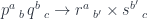
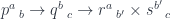
and a heteromorphism $h \in P(c, d)$ . Their composition is another heteromorphism obtained by lifting the pair $(f, id_d)$ . Indeed:

$P(f, id_d) \colon P(c, d) \to P(c', d)$

so its action on $h$ produces a heteromorphism from $c'$ to $d$ , which we can call the composition $h \circ f$ of a heteromorphism $h$ with a morphism $f$ . Similarly, a morphism in $\mathbb{D}$ :

$g\colon d \to d'$

can be composed with $h$ by lifting $(id_c, g)$ .

In Haskell, this new composition would be implemented by applying dimap f id to precompose p c d with

f :: c' -> c

and dimap id g to postcompose it with

g :: d -> d'

This is how we can use a profunctor to glue together two categories. Two categories connected by a profunctor form a new category known as their collage.

A given profunctor provides unidirectional flow of heteromorphisms from $\mathbb{C}$ to $\mathbb{D}$ , so there is no opportunity to compose two heteromorphisms.

Profunctors As Relations

The opportunity to compose heteromorphisms arises when we decide to glue more than two categories. The clue as how to proceed comes from yet another interpretation of profunctors: as proof-relevant relations. In classical logic, a relation between sets assigns a Boolean true or false to each pair of elements. The elements are either related or not, period. In proof-relevant logic, we are not only interested in whether something is true, but also in gathering witnesses to the proofs. So, instead of assigning a single Boolean to each pair of elements, we assign a whole set. If the set is empty, the elements are unrelated. If it’s non-empty, each element is a separate witness to the relation.

This definition of a relation can be generalized to any category. In fact there is already a natural relation between objects in a category–the one defined by hom-sets. Two objects $a$ and $b$ are related this way if the hom-set $C(a, b)$ is non-empty. Each morphism in $C(a, b)$ serves as a witness to this relation.

With profunctors, we can define proof-relevant relations between objects that are taken from different categories. Object $c$ in $\mathbb{C}$ is related to object $d$ in $\mathbb{D}$ if $P(c, d)$ is a non-empty set. Moreover, each element of this set serves as a witness for the relation. Because of functoriality of $P$ , this relation is compatible with the categorical structure, that is, it composes nicely with the relation defined by hom-sets.

In general, a composition of two relations $P$ and $Q$ , denoted by $P \circ Q$ is defined as a path between objects. Objects $a$ and $c$ are related if there is a go-between object $b$ such that both $P(a, b)$ and $Q(b, c)$ are non-empty. As a witness of this relation we can pick any pair of elements, one from $P(a, b)$ and one from $Q(b, c)$ .

By convention, a profunctor $P(a, b)$ is drawn as an arrow (often crossed) from $b$ to $a$ , $a \nleftarrow b$ .

Composition of profunctors/relations

Profunctor Composition

To create a set of all witnesses of $P \circ Q$ we have to sum over all possible intermediate objects and all pairs of witnesses. Roughly speaking, such a sum (modulo some identifications) is expressed categorically as a coend:

$(P \circ Q)(a, c) = \int^b P(a, b) \times Q(b, c)$

As a refresher, a coend of a profunctor $P$ is a set $\int^a P(a, a)$ equipped with a family of injections

$i_x \colon P(x, x) \to \int^a P(a, a)$

that is universal in the sense that, for any other set $s$ and a family:

$\alpha_x \colon P(x, x) \to s$

there is a unique function $h$ that factorizes them all:

$\alpha_x = h \circ i_x$

Universal property of a coend

Profunctor composition can be translated into pseudo-Haskell as:

type Procompose q p a c = exists b. (p a b, q b c)

where the coend is encoded as an existential data type. The actual implementation (again, see Edward Kmett’s Data.Profunctor.Composition) is:

data Procompose q p a c where
  Procompose :: q b c -> p a b -> Procompose q p a c

The existential quantifier is expressed in terms of a GADT (Generalized Algebraic Data Type), with the free occurrence of b inside the data constructor.

Einstein’s Convention

By now you might be getting lost juggling the variances of objects appearing in those formulas. The coend variable, for instance, must appear under the integral sign once in the covariant and once in the contravariant position, and the variances on the right must match the variances on the left. Fortunately, there is a precedent in a different branch of mathematics, tensor calculus in vector spaces, with the kind of notation that takes care of variances. Einstein coopted and expanded this notation in his theory of relativity. Let’s see if we can adapt this technique to the calculus of profunctors.

The trick is to write contravariant indices as superscripts and the covariant ones as subscripts. So, from now on, we’ll write the components of a profunctor $p$ (we’ll switch to lower case to be compatible with Haskell) as $p^c\,_d$ . Einstein also came up with a clever convention: implicit summation over a repeated index. In the case of profunctors, the summation corresponds to taking a coend. In this notation, a coend over a profunctor $p$ looks like a trace of a tensor:

$p^a\,_a = \int^a p(a, a)$

The composition of two profunctors becomes:

$(p \circ q)^a\, _c = p^a\,_b \, q^b\,_c = \int^b p(a, b) \times q(b, c)$

The summation convention applies only to adjacent indices. When they are separated by an explicit product sign (or any other operator), the coend is not assumed, as in:

$p^a\,_b \times q^b\,_c$

(no summation).

The hom-functor in a category $\mathbb{C}$ is also a profunctor, so it can be notated appropriately:

$C^a\,_b = C(a, b)$

The co-Yoneda lemma (see Ninja Yoneda) becomes:

$C^c\,_{c'}\,p^{c'}\,_d \cong p^c\,_d \cong p^c\,_{d'}\,D^{d'}\,_d$

suggesting that the hom-functors $C^c\,_{c'}$ and $D^{d'}\,_d$ behave like Kronecker deltas (in tensor-speak) or unit matrices. Here, the profunctor $p$ spans two categories

$p \colon \mathbb{C}^{op}\times \mathbb{D} \to Set$

The lifting of morphisms:

$f\colon c' \to c$
$g\colon d \to d'$

can be written as:

$p^f\,_g \colon p^c\,_d \to p^{c'}\,_{d'}$

There is one more useful identity that deals with mapping out from a coend. It’s the consequence of the fact that the hom-functor is continuous. It means that it maps (co-) limits to limits. More precisely, since the hom-functor is contravariant in the first variable, when we fix the target object, it maps colimits in the first variable to limits. (It also maps limits to limits in the second variable). Since a coend is a colimit, and an end is a limit, continuity leads to the following identity:

$Set(\int^c p(c, c), s) \cong \int_c Set(p(c, c), s)$

for any set $s$ . Programmers know this identity as a generalization of case analysis: a function from a sum type is a product of functions (one function per case). If we interpret the coend as an existential quantifier, the end is equivalent to a universal quantifier.

Let’s apply this identity to the mapping out from a composition of two profunctors:

$p^a\,_b \, q^b\,_c \to s = Set\big(\int^b p(a, b) \times q(b, c), s\big)$

This is isomorphic to:

$\int_b Set\Big(p(a,b) \times q(b, c), s\Big)$

or, after currying (using the product/exponential adjunction),

$\int_b Set\Big(p(a, b), q(b, c) \to s\Big)$

This gives us the mapping out formula:

$p^a\,_b \, q^b\,_c \to s \cong p^a\,_b \to q^b\,_c \to s$

with the right hand side natural in $b$ . Again, we don’t perform implicit summation on the right, where the repeated indices are separated by an arrow. There, the repeated index $b$ is universally quantified (through the end), giving rise to a natural transformation.

Bicategory Prof

Since profunctors can be composed using the coend formula, it’s natural to ask if there is a category in which they work as morphisms. The only problem is that profunctor composition satisfies the associativity and unit laws (see the co-Yoneda lemma above) only up to isomorphism. Not to worry, there is a name for that: a bicategory. In a bicategory we have objects, which are called 0-cells; morphisms, which are called 1-cells; and morphisms between morphisms, which are called 2-cells. When we say that categorical laws are satisfied up to isomorphism, it means that there is an invertible 2-cell that maps one side of the law to another.

The bicategory $Prof$ has categories as 0-cells, profunctors as 1-cells, and natural transformations as 2-cells. A natural transformation $\alpha$ between profunctors $p$ and $q$

$\alpha \colon p \Rightarrow q$

has components that are functions:

$\alpha^c\,_d \colon p^c\,_d \to q^c\,_d$

satisfying the usual naturality conditions. Natural transformations between profunctors can be composed as functions (this is called vertical composition). In fact 2-cells in any bicategory are composable, and there always is a unit 2-cell. It follows that 1-cells between any two 0-cells form a category called the hom-category.

But there is another way of composing 2-cells that’s called horizontal composition. In $Prof$ , this horizontal composition is not the usual horizontal composition of natural transformations, because composition of profunctors is not the usual composition of functors. We have to construct a natural transformation between one composition of profuntors, say $p^a\,_b \, q^b\,_c$ and another, $r^a\,_b \, s^b\,_c$ , having at our disposal two natural transformations:

$\alpha \colon p \Rightarrow r$

$\beta \colon q \Rightarrow s$

The construction is a little technical, so I’m moving it to the appendix. We will denote such horizontal composition as:

$(\alpha \circ \beta)^a\,_c \colon p^a\,_b \, q^b\,_c \to r^a\,_b \, s^b\,_c$

If one of the natural transformations is an identity natural transformation, say, from $p^a\,_b$ to $p^a\,_b$ , horizontal composition is called whiskering and can be written as:

$(p \circ \beta)^a\,_c \colon p^a\,_b \, q^b\,_c \to p^a\,_b \, s^b\,_c$

Promonads

The fact that a monad is a monoid in the category of endofunctors is a lucky accident. That’s because, in general, a monad can be defined in any bicategory, and $Cat$ just happens to be a (strict) bicategory. It has (small) categories as 0-cells, functors as 1-cells, and natural transformations as 2-cells. A monad is defined as a combination of a 0-cell (you need a category to define a monad), an endo-1-cell (that would be an endofunctor in that category), and two 2-cells. These 2-cells are variably called multiplication and unit, $\mu$ and $\eta$ , or join and return.

Since $Prof$ is a bicategory, we can define a monad in it, and call it a promonad. A promonad consists of a 0-cell $C$ , which is a category; an endo-1-cell $p$ , which is a profunctor in that category; and two 2-cells, which are natural transformations:

$\mu^a\,_b \colon p^a\,_c \, p^c\,_b \to p^a\,_b$

$\eta^a\,_b \colon C^a\,_b \to p^a\,_b$

Remember that $C^a\,_b$ is the hom-profunctor in the category $C$ which, due to co-Yoneda, happens to be the unit of profunctor composition.

Programmers might recognize elements of the Haskell Arrow in it (see my blog post on monoids).

We can apply the mapping-out identity to the definition of multiplication and get:

$\mu^a\,_b \colon p^a\,_c \to p^c\,_b \to p^a\,_b$

Notice that this looks very much like composition of heteromorphisms. Moreover, the monadic unit $\eta$ maps regular morphisms to heteromorphisms. We can then construct a new category, whose objects are the same as the objects of $\mathbb{C}$ , with hom-sets given by the profunctor $p$ . That is, a hom set from $a$ to $b$ is the set $p^a\,_b$ . We can define an identity-on-object functor $J$ from $\mathbb{C}$ to that category, whose action on hom-sets is given by $\eta$ .

Interestingly, this construction also works in the opposite direction (as was brought to my attention by Alex Campbell). Any indentity-on-objects functor defines a promonad. Indeed, given a functor $J$ , we can always turn it into a profunctor:

$p(c, d) = D(J\, c, J\, d)$

In Einstein notation, this reads:

$p^c\,_d = D^{J\, c}\,_{J\, d}$

Since $J$ is identity on objects, the composition of morphisms in $D$ can be used to define the composition of heteromorphisms. This, in turn, can be used to define $\mu$ , thus showing that $p$ is a promonad on $\mathbb{C}$ .

Conclusion

I realize that I have touched upon some pretty advanced topics in category theory, like bicategories and promonads, so it’s a little surprising that these concepts can be illustrated in Haskell, some of them being present in popular libraries, like the Arrow library, which has applications in functional reactive programming.

I’ve been experimenting with applying Einstein’s summation convention to profunctors, admittedly with mixed results. This is definitely work in progress and I welcome suggestions to improve it. The main problem is that we sometimes need to apply the sum (coend), and at other times the product (end) to repeated indices. This is in particular awkward in the formulation of the mapping out property. I suggest separating the non-summed indices with product signs or arrows but I’m not sure how well this will work.

Appendix: Horizontal Composition in Prof

We have at our disposal two natural transformations:

$\alpha \colon p \Rightarrow r$

$\beta \colon q \Rightarrow s$

and the following coend, which is the composition of the profunctors $p$ and $q$ :

$\int^b p(a, b) \times q(b, c)$

Our goal is to construct an element of the target coend:

$\int^b r(a, b) \times s(b, c)$

Horizontal composition of 2-cells

To construct an element of a coend, we need to provide just one element of $r(a, b') \times s(b', c)$ for some $b'$ . We’ll look for a function that would construct such an element in the following hom-set:

$Set\Big(\int^b p(a, b) \times q(b, c), r(a, b') \times s(b', c)\Big)$

Using Einstein notation, we can write it as:

$p^a\,_b \, q^b\,_c \to r^a\,_{b'} \times s^{b'}\,_c$

and then use the mapping out property:

$p^a\,_b \to q^b\,_c \to r^a\,_{b'} \times s^{b'}\,_c$

We can pick $b'$ equal to $b$ and implement the function using the components of the two natural transformations, $\alpha^a\,_{b} \times \beta^{b}\,_c$ .

Of course, this is how a programmer might think of it. A mathematician will use the universal property of the coend $(p \circ q)^a\,_c$ , as in the diagram below (courtesy Alex Campbell).

Horizontal composition using the universal property of a coend

In Haskell, we can define a natural transformation between two (endo-) profunctors as a polymorphic function:

newtype PNat p q = PNat (forall a b. p a b -> q a b)

Horizontal composition is then given by:

horPNat :: PNat p r -> PNat q s -> Procompose p q a c
        -> Procompose r s a c
horPNat (PNat alpha) (PNat beta) (Procompose pbc qdb) = 
  Procompose (alpha pbc) (beta qdb)

Acknowledgment

I’m grateful to Alex Campbell from Macquarie University in Sydney for extensive help with this blog post.

Recursion Schemes for Higher Algebras

Posted by Bartosz Milewski under Category Theory, Functional Programming, Haskell, Monads, Programming
[4] Comments

Abstract

The use of free monads, free applicatives, and cofree comonads lets us separate the construction of (often effectful or context-dependent) computations from their interpretation. In this paper I show how the ad hoc process of writing interpreters for these free constructions can be systematized using the language of higher order algebras (coalgebras) and catamorphisms (anamorphisms).

Introduction

Recursive schemes [meijer] are an example of successful application of concepts from category theory to programming. The idea is that recursive data structures can be defined as initial algebras of functors. This allows a separation of concerns: the functor describes the local shape of the data structure, and the fixed point combinator builds the recursion. Operations over data structures can be likewise separated into shallow, non-recursive computations described by algebras, and generic recursive procedures described by catamorphisms. In this way, data structures often replace control structures in driving computations.

Since functors also form a category, it’s possible to define functors acting on functors. Such higher order functors show up in a number of free constructions, notably free monads, free applicatives, and cofree comonads. These free constructions have good composability properties and they provide means of separating the creation of effectful computations from their interpretation.

This paper’s contribution is to systematize the construction of such interpreters. The idea is that free constructions arise as fixed points of higher order functors, and therefore can be approached with the same algebraic machinery as recursive data structures, only at a higher level. In particular, interpreters can be constructed as catamorphisms or anamorphisms of higher order algebras/coalgebras.

Initial Algebras and Catamorphisms

The canonical example of a data structure that can be described as an initial algebra of a functor is a list. In Haskell, a list can be defined recursively:

data List a = Nil | Cons a (List a)

There is an underlying non-recursive functor:

data ListF a x = NilF | ConsF a x
instance Functor (ListF a) where
  fmap f NilF = NilF
  fmap f (ConsF a x) = ConsF a (f x)

Once we have a functor, we can define its algebras. An algebra consist of a carrier c and a structure map (evaluator). An algebra can be defined for an arbitrary functor f:

type Algebra f c = f c -> c

Here’s an example of a simple list algebra, with Int as its carrier:

sum :: Algebra (ListF Int) Int
sum NilF = 0
sum (ConsF a c) = a + c

Algebras for a given functor form a category. The initial object in this category (if it exists) is called the initial algebra. In Haskell, we call the carrier of the initial algebra Fix f. Its structure map is a function:

f (Fix f) -> Fix f

By Lambek’s lemma, the structure map of the initial algebra is an isomorphism. In Haskell, this isomorphism is given by a pair of functions: the constructor In and the destructor out of the fixed point combinator:

newtype Fix f = In { out :: f (Fix f) }

When applied to the list functor, the fixed point gives rise to an alternative definition of a list:

type List a = Fix (ListF a)

The initiality of the algebra means that there is a unique algebra morphism from it to any other algebra. This morphism is called a catamorphism and, in Haskell, can be expressed as:

cata :: Functor f => Algebra f a -> Fix f -> a
cata alg = alg . fmap (cata alg) . out

A list catamorphism is known as a fold. Since the list functor is a sum type, its algebra consists of a value—the result of applying the algebra to NilF—and a function of two variables that corresponds to the ConsF constructor. You may recognize those two as the arguments to foldr:

foldr :: (a -> c -> c) -> c -> [a] -> c

The list functor is interesting because its fixed point is a free monoid. In category theory, monoids are special objects in monoidal categories—that is categories that define a product of two objects. In Haskell, a pair type plays the role of such a product, with the unit type as its unit (up to isomorphism).

As you can see, the list functor is the sum of a unit and a product. This formula can be generalized to an arbitrary monoidal category with a tensor product $\otimes$ and a unit $1$ :

$L\, a\, x = 1 + a \otimes x$

Its initial algebra is a free monoid .

Higher Algebras

In category theory, once you performed a construction in one category, it’s easy to perform it in another category that shares similar properties. In Haskell, this might require reimplementing the construction.

We are interested in the category of endofunctors, where objects are endofunctors and morphisms are natural transformations. Natural transformations are represented in Haskell as polymorphic functions:

type f :~> g = forall a. f a -> g a
infixr 0 :~>

In the category of endofunctors we can define (higher order) functors, which map functors to functors and natural transformations to natural transformations:

class HFunctor hf where
  hfmap :: (g :~> h) -> (hf g :~> hf h)
  ffmap :: Functor g => (a -> b) -> hf g a -> hf g b

The first function lifts a natural transformation; and the second function, ffmap, witnesses the fact that the result of a higher order functor is again a functor.

An algebra for a higher order functor hf consists of a functor f (the carrier object in the functor category) and a natural transformation (the structure map):

type HAlgebra hf f = hf f :~> f

As with regular functors, we can define an initial algebra using the fixed point combinator for higher order functors:

newtype FixH hf a = InH { outH :: hf (FixH hf) a }

Similarly, we can define a higher order catamorphism:

hcata :: HFunctor h => HAlgebra h f -> FixH h :~> f
hcata halg = halg . hfmap (hcata halg) . outH

The question is, are there any interesting examples of higher order functors and algebras that could be used to solve real-life programming problems?

Free Monad

We’ve seen the usefulness of lists, or free monoids, for structuring computations. Let’s see if we can generalize this concept to higher order functors.

The definition of a list relies on the monoidal structure of the underlying category. It turns out that there are multiple monoidal structures of interest that can be defined in the category of functors. The simplest one defines a product of two endofunctors as their composition. Any two endofunctors can be composed. The unit of functor composition is the identity functor.

If you picture endofunctors as containers, you can easily imagine a tree of lists, or a list of Maybes.

A monoid based on this particular monoidal structure in the endofunctor category is a monad. It’s an endofunctor m equipped with two natural transformations representing unit and multiplication:

class Monad m where
  eta :: Identity    :~> m
  mu  :: Compose m m :~> m

In Haskell, the components of these natural transformations are known as return and join.

A straightforward generalization of the list functor to the functor category can be written as:

$L\, f\, g = 1 + f \circ g$

or, in Haskell,

type FunctorList f g = Identity :+: Compose f g

where we used the operator :+: to define the coproduct of two functors:

data (f :+: g) e = Inl (f e) | Inr (g e)
infixr 7 :+:

Using more conventional notation, FunctorList can be written as:

data MonadF f g a = 
    DoneM a 
  | MoreM (f (g a))

We’ll use it to generate a free monoid in the category of endofunctors. First of all, let’s show that it’s indeed a higher order functor in the second argument g:

instance Functor f => HFunctor (MonadF f) where
  hfmap _   (DoneM a)  = DoneM a
  hfmap nat (MoreM fg) = MoreM $ fmap nat fg
  ffmap h (DoneM a)    = DoneM (h a)
  ffmap h (MoreM fg)   = MoreM $ fmap (fmap h) fg

In category theory, because of size issues, this functor doesn’t always have a fixed point. For most common choices of f (e.g., for algebraic data types), the initial higher order algebra for this functor exists, and it generates a free monad. In Haskell, this free monad can be defined as:

type FreeMonad f = FixH (MonadF f)

We can show that FreeMonad is indeed a monad by implementing return and bind:

instance Functor f => Monad (FreeMonad f) where
  return = InH . DoneM
  (InH (DoneM a))    >>= k = k a
  (InH (MoreM ffra)) >>= k = 
        InH (MoreM (fmap (>>= k) ffra))

Free monads have many applications in programming. They can be used to write generic monadic code, which can then be interpreted in different monads. A very useful property of free monads is that they can be composed using coproducts. This follows from the theorem in category theory, which states that left adjoints preserve coproducts (or, more generally, colimits). Free constructions are, by definition, left adjoints to forgetful functors. This property of free monads was explored by Swierstra [swierstra] in his solution to the expression problem. I will use an example based on his paper to show how to construct monadic interpreters using higher order catamorphisms.

Free Monad Example

A stack-based calculator can be implemented directly using the state monad. Since this is a very simple example, it will be instructive to re-implement it using the free monad approach.

We start by defining a functor, in which the free parameter k represents the continuation:

data StackF k  = Push Int k
               | Top (Int -> k)
               | Pop k            
               | Add k
               deriving Functor

We use this functor to build a free monad:

type FreeStack = FreeMonad StackF

You may think of the free monad as a tree with nodes that are defined by the functor StackF. The unary constructors, like Add or Pop, create linear list-like branches; but the Top constructor branches out with one child per integer.

The level of indirection we get by separating recursion from the functor makes constructing free monad trees syntactically challenging, so it makes sense to define a helper function:

liftF :: (Functor f) => f r -> FreeMonad f r
liftF fr = InH $ MoreM $ fmap (InH . DoneM) fr

With this function, we can define smart constructors that build leaves of the free monad tree:

push :: Int -> FreeStack ()
push n = liftF (Push n ())

pop :: FreeStack ()
pop = liftF (Pop ())

top :: FreeStack Int
top = liftF (Top id)

add :: FreeStack ()
add = liftF (Add ())

All these preparations finally pay off when we are able to create small programs using do notation:

calc :: FreeStack Int
calc = do
  push 3
  push 4
  add
  x <- top
  pop
  return x

Of course, this program does nothing but build a tree. We need a separate interpreter to do the calculation. We’ll interpret our program in the state monad, with state implemented as a stack (list) of integers:

type MemState = State [Int]

The trick is to define a higher order algebra for the functor that generates the free monad and then use a catamorphism to apply it to the program. Notice that implementing the algebra is a relatively simple procedure because we don’t have to deal with recursion. All we need is to case-analyze the shallow constructors for the free monad functor MonadF, and then case-analyze the shallow constructors for the functor StackF.

runAlg :: HAlgebra (MonadF StackF) MemState
runAlg (DoneM a)  = return a
runAlg (MoreM ex) = 
  case ex of
    Top  ik  -> get >>= ik  . head
    Pop  k   -> get >>= put . tail   >> k
    Push n k -> get >>= put . (n : ) >> k
    Add  k   -> do (a: b: s) <- get
                   put (a + b : s)
                   k

The catamorphism converts the program calc into a state monad action, which can be run over an empty initial stack:

runState (hcata runAlg calc) []

The real bonus is the freedom to define other interpreters by simply switching the algebras. Here’s an algebra whose carrier is the Const functor:

showAlg :: HAlgebra (MonadF StackF) (Const String)

showAlg (DoneM a) = Const "Done!"
showAlg (MoreM ex) = Const $
  case ex of
    Push n k -> 
      "Push " ++ show n ++ ", " ++ getConst k
    Top ik -> 
      "Top, " ++ getConst (ik 42)
    Pop k -> 
      "Pop, " ++ getConst k
    Add k -> 
      "Add, " ++ getConst k

Runing the catamorphism over this algebra will produce a listing of our program:

getConst $ hcata showAlg calc

> "Push 3, Push 4, Add, Top, Pop, Done!"

Free Applicative

There is another monoidal structure that exists in the category of functors. In general, this structure will work for functors from an arbitrary monoidal category $C$ to $Set$ . Here, we’ll restrict ourselves to endofunctors on $Set$ . The product of two functors is given by Day convolution, which can be implemented in Haskell using an existential type:

data Day f g c where
  Day :: f a -> g b -> ((a, b) -> c) -> Day f g c

The intuition is that a Day convolution contains a container of some as, and another container of some bs, together with a function that can convert any pair (a, b) to c.

Day convolution is a higher order functor:

instance HFunctor (Day f) where
  hfmap nat (Day fx gy xyt) = Day fx (nat gy) xyt
  ffmap h   (Day fx gy xyt) = Day fx gy (h . xyt)

In fact, because Day convolution is symmetric up to isomorphism, it is automatically functorial in both arguments.

To complete the monoidal structure, we also need a functor that could serve as a unit with respect to Day convolution. In general, this would be the the hom-functor from the monoidal unit:

$C(1, -)$

In our case, since $1$ is the singleton set, this functor reduces to the identity functor.

We can now define monoids in the category of functors with the monoidal structure given by Day convolution. These monoids are equivalent to lax monoidal functors which, in Haskell, form the class:

class Functor f => Monoidal f where
  unit  :: f ()
  (>*<) :: f x -> f y -> f (x, y)

Lax monoidal functors are equivalent to applicative functors [mcbride], as seen in this implementation of pure and <*>:

  pure  :: a -> f a
  pure a = fmap (const a) unit
  (<*>) :: f (a -> b) -> f a -> f b
  fs <*> as = fmap (uncurry ($)) (fs >*< as)

We can now use the same general formula, but with Day convolution as the product:

$L\, f\, g = 1 + f \star g$

to generate a free monoidal (applicative) functor:

data FreeF f g t =
      DoneF t
    | MoreF (Day f g t)

This is indeed a higher order functor:

instance HFunctor (FreeF f) where
    hfmap _ (DoneF x)     = DoneF x
    hfmap nat (MoreF day) = MoreF (hfmap nat day)
    ffmap f (DoneF x)     = DoneF (f x)
    ffmap f (MoreF day)   = MoreF (ffmap f day)

and it generates a free applicative functor as its initial algebra:

type FreeA f = FixH (FreeF f)

Free Applicative Example

The following example is taken from the paper by Capriotti and Kaposi [capriotti]. It’s an option parser for a command line tool, whose result is a user record of the following form:

data User = User
  { username :: String 
  , fullname :: String
  , uid      :: Int
  } deriving Show

A parser for an individual option is described by a functor that contains the name of the option, an optional default value for it, and a reader from string:

data Option a = Option
  { optName    :: String
  , optDefault :: Maybe a
  , optReader  :: String -> Maybe a 
  } deriving Functor

Since we don’t want to commit to a particular parser, we’ll create a parsing action using a free applicative functor:

userP :: FreeA Option User
userP  = pure User 
  <*> one (Option "username" (Just "John")  Just)
  <*> one (Option "fullname" (Just "Doe")   Just)
  <*> one (Option "uid"      (Just 0)       readInt)

where readInt is a reader of integers:

readInt :: String -> Maybe Int
readInt s = readMaybe s

and we used the following smart constructors:

one :: f a -> FreeA f a
one fa = InH $ MoreF $ Day fa (done ()) fst

done :: a -> FreeA f a
done a = InH $ DoneF a

We are now free to define different algebras to evaluate the free applicative expressions. Here’s one that collects all the defaults:

alg :: HAlgebra (FreeF Option) Maybe
alg (DoneF a) = Just a
alg (MoreF (Day oa mb f)) = 
  fmap f (optDefault oa >*< mb)

I used the monoidal instance for Maybe:

instance Monoidal Maybe where
  unit = Just ()
  Just x >*< Just y = Just (x, y)
  _ >*< _ = Nothing

This algebra can be run over our little program using a catamorphism:

parserDef :: FreeA Option a -> Maybe a
parserDef = hcata alg

And here’s an algebra that collects the names of all the options:

alg2 :: HAlgebra (FreeF Option) (Const String)
alg2 (DoneF a) = Const "."
alg2 (MoreF (Day oa bs f)) = 
  fmap f (Const (optName oa) >*< bs)

Again, this uses a monoidal instance for Const:

instance Monoid m => Monoidal (Const m) where
  unit = Const mempty
  Const a >*< Const b = Const (a  b)

We can also define the Monoidal instance for IO:

instance Monoidal IO where
  unit = return ()
  ax >*< ay = do a <- ax
                 b <- ay
                 return (a, b)

This allows us to interpret the parser in the IO monad:

alg3 :: HAlgebra (FreeF Option) IO
alg3 (DoneF a) = return a
alg3 (MoreF (Day oa bs f)) = do
    putStrLn $ optName oa
    s <- getLine
    let ma = optReader oa s
        a = fromMaybe (fromJust (optDefault oa)) ma
    fmap f $ return a >*< bs

Cofree Comonad

Every construction in category theory has its dual—the result of reversing all the arrows. The dual of a product is a coproduct, the dual of an algebra is a coalgebra, and the dual of a monad is a comonad.

Let’s start by defining a higher order coalgebra consisting of a carrier f, which is a functor, and a natural transformation:

type HCoalgebra hf f = f :~> hf f

An initial algebra is dualized to a terminal coalgebra. In Haskell, both are the results of applying the same fixed point combinator, reflecting the fact that the Lambek’s lemma is self-dual. The dual to a catamorphism is an anamorphism. Here is its higher order version:

hana :: HFunctor hf 
     => HCoalgebra hf f -> (f :~> FixH hf)
hana hcoa = InH . hfmap (hana hcoa) . hcoa

The formula we used to generate free monoids:

$1 + a \otimes x$

dualizes to:

$1 \times a \otimes x$

and can be used to generate cofree comonoids .

A cofree functor is the right adjoint to the forgetful functor. Just like the left adjoint preserved coproducts, the right adjoint preserves products. One can therefore easily combine comonads using products (if the need arises to solve the coexpression problem).

Just like the monad is a monoid in the category of endofunctors, a comonad is a comonoid in the same category. The functor that generates a cofree comonad has the form:

type ComonadF f g = Identity :*: Compose f g

where the product of functors is defined as:

data (f :*: g) e = Both (f e) (g e)
infixr 6 :*:

Here’s the more familiar form of this functor:

data ComonadF f g e = e :< f (g e)

It is indeed a higher order functor, as witnessed by this instance:

instance Functor f => HFunctor (ComonadF f) where
  hfmap nat (e :< fge) = e :< fmap nat fge
  ffmap h (e :< fge) = h e :< fmap (fmap h) fge

A cofree comonad is the terminal coalgebra for this functor and can be written as a fixed point:

type Cofree f = FixH (ComonadF f)

Indeed, for any functor f, Cofree f is a comonad:

instance Functor f => Comonad (Cofree f) where
  extract (InH (e :< fge)) = e
  duplicate fr@(InH (e :< fge)) = 
                InH (fr :< fmap duplicate fge)

Cofree Comonad Example

The canonical example of a cofree comonad is an infinite stream:

type Stream = Cofree Identity

We can use this stream to sample a function. We’ll encapsulate this function inside the following functor (in fact, itself a comonad):

data Store a x = Store a (a -> x) 
    deriving Functor

We can use a higher order coalgebra to unpack the Store into a stream:

streamCoa :: HCoalgebra (ComonadF Identity)(Store Int)
streamCoa (Store n f) = 
    f n :< (Identity $ Store (n + 1) f)

The actual unpacking is a higher order anamorphism:

stream :: Store Int a -> Stream a
stream = hana streamCoa

We can use it, for instance, to generate a list of squares of natural numbers:

stream (Store 0 (^2))

Since, in Haskell, the same fixed point defines a terminal coalgebra as well as an initial algebra, we are free to construct algebras and catamorphisms for streams. Here’s an algebra that converts a stream to an infinite list:

listAlg :: HAlgebra (ComonadF Identity) []
listAlg(a :< Identity as) = a : as

toList :: Stream a -> [a]
toList = hcata listAlg

Future Directions

In this paper I concentrated on one type of higher order functor:

$1 + a \otimes x$

and its dual. This would be equivalent to studying folds for lists and unfolds for streams. But the structure of the functor category is richer than that. Just like basic data types can be combined into algebraic data types, so can functors. Moreover, besides the usual sums and products, the functor category admits at least two additional monoidal structures generated by functor composition and Day convolution.

Another potentially fruitful area of exploration is the profunctor category, which is also equipped with two monoidal structures, one defined by profunctor composition, and another by Day convolution. A free monoid with respect to profunctor composition is the basis of Haskell Arrow library [jaskelioff]. Profunctors also play an important role in the Haskell lens library [kmett].

Bibliography

Erik Meijer, Maarten Fokkinga, and Ross Paterson, Functional Programming with Bananas, Lenses, Envelopes and Barbed Wire
Conor McBride, Ross Paterson, Idioms: applicative programming with effects
Paolo Capriotti, Ambrus Kaposi, Free Applicative Functors
Wouter Swierstra, Data types a la carte
Exequiel Rivas and Mauro Jaskelioff, Notions of Computation as Monoids
Edward Kmett, Lenses, Folds and Traversals
Richard Bird and Lambert Meertens, Nested Datatypes
Patricia Johann and Neil Ghani, Initial Algebra Semantics is Enough!

March 14, 2017

Algebras for Monads

Posted by Bartosz Milewski under Category Theory, Monads
[12] Comments

This is part 25 of Categories for Programmers. Previously: F-Algebras. See the Table of Contents.

If we interpret endofunctors as ways of defining expressions, algebras let us evaluate them and monads let us form and manipulate them. By combining algebras with monads we not only gain a lot of functionality but we can also answer a few interesting questions. One such question concerns the relation between monads and adjunctions. As we’ve seen, every adjunction defines a monad (and a comonad). The question is: Can every monad (comonad) be derived from an adjunction? The answer is positive. There is a whole family of adjunctions that generate a given monad. I’ll show you two such adjunction.

Let’s review the definitions. A monad is an endofunctor m equipped with two natural transformations that satisfy some coherence conditions. The components of these transformations at a are:

η_a :: a -> m a
μ_a :: m (m a) -> m a

An algebra for the same endofunctor is a selection of a particular object — the carrier a — together with the morphism:

alg :: m a -> a

The first thing to notice is that the algebra goes in the opposite direction to η_a. The intuition is that η_a creates a trivial expression from a value of type a. The first coherence condition that makes the algebra compatible with the monad ensures that evaluating this expression using the algebra whose carrier is a gives us back the original value:

alg ∘ η_a = id_a

The second condition arises from the fact that there are two ways of evaluating the doubly nested expression m (m a). We can first apply μ_a to flatten the expression, and then use the evaluator of the algebra; or we can apply the lifted evaluator to evaluate the inner expressions, and then apply the evaluator to the result. We’d like the two strategies to be equivalent:

alg ∘ μ_a = alg ∘ m alg

Here, m alg is the morphism resulting from lifting alg using the functor m. The following commuting diagrams describe the two conditions (I replaced m with T in anticipation of what follows):

We can also express these condition in Haskell:

alg . return = id
alg . join = alg . fmap alg

Let’s look at a small example. An algebra for a list endofunctor consists of some type a and a function that produces an a from a list of a. We can express this function using foldr by choosing both the element type and the accumulator type to be equal to a:

foldr :: (a -> a -> a) -> a -> [a] -> a

This particular algebra is specified by a two-argument function, let’s call it f, and a value z. The list functor happens to also be a monad, with return turning a value into a singleton list. The composition of the algebra, here foldr f z, after return takes x to:

foldr f z [x] = x `f` z

where the action of f is written in the infix notation. The algebra is compatible with the monad if the following coherence condition is satisfied for every x:

x `f` z = x

If we look at f as a binary operator, this condition tells us that z is the right unit.

The second coherence condition operates on a list of lists. The action of join concatenates the individual lists. We can then fold the resulting list. On the other hand, we can first fold the individual lists, and then fold the resulting list. Again, if we interpret f as a binary operator, this condition tells us that this binary operation is associative. These conditions are certainly fulfilled when (a, f, z) is a monoid.

T-algebras

Since mathematicians prefer to call their monads T, they call algebras compatible with them T-algebras. T-algebras for a given monad T in a category C form a category called the Eilenberg-Moore category, often denoted by C^T. Morphisms in that category are homomorphisms of algebras. These are the same homomorphisms we’ve seen defined for F-algebras.

A T-algebra is a pair consisting of a carrier object and an evaluator, (a, f). There is an obvious forgetful functor U^T from C^T to C, which maps (a, f) to a. It also maps a homomorphism of T-algebras to a corresponding morphism between carrier objects in C. You may remember from our discussion of adjunctions that the left adjoint to a forgetful functor is called a free functor.

The left adjoint to U^T is called F^T. It maps an object a in C to a free algebra in C^T. The carrier of this free algebra is T a. Its evaluator is a morphism from T (T a) back to T a. Since T is a monad, we can use the monadic μ_a (Haskell join) as the evaluator.

We still have to show that this is a T-algebra. For that, two coherence conditions must be satisified:

alg ∘ η_Ta = id_Ta

alg ∘ μ_a = alg ∘ T alg

But these are just monadic laws, if you plug in μ for the algebra.

As you may recall, every adjunction defines a monad. It turns out that the adjunction between F^T and U^T defines the very monad T that was used in the construction of the Eilenberg-Moore category. Since we can perform this construction for every monad, we conclude that every monad can be generated from an adjunction. Later I’ll show you that there is another adjunction that generates the same monad.

Here’s the plan: First I’ll show you that F^T is indeed the left adjoint of U^T. I’ll do it by defining the unit and the counit of this adjunction and proving that the corresponding triangular identities are satisfied. Then I’ll show you that the monad generated by this adjunction is indeed our original monad.

The unit of the adjunction is the natural transformation:

η :: I -> U^T ∘ F^T

Let’s calculate the a component of this transformation. The identity functor gives us a. The free functor produces the free algebra (T a, μ_a), and the forgetful functor reduces it to T a. Altogether we get a mapping from a to T a. We’ll simply use the unit of the monad T as the unit of this adjunction.

Let’s look at the counit:

ε :: F^T ∘ U^T -> I

Let’s calculate its component at some T-algebra (a, f). The forgetful functor forgets the f, and the free functor produces the pair (T a, μ_a). So in order to define the component of the counit ε at (a, f), we need the right morphism in the Eilenberg-Moore category, or a homomorphism of T-algebras:

(T a, μ_a) -> (a, f)

Such homomorphism should map the carrier T a to a. Let’s just resurrect the forgotten evaluator f. This time we’ll use it as a homomorphism of T-algebras. Indeed, the same commuting diagram that makes f a T-algebra may be re-interpreted to show that it’s a homomorphism of T-algebras:

We have thus defined the component of the counit natural transformation ε at (a, f) (an object in the category of T-algebras) to be f.

To complete the adjunction we also need to show that the unit and the counit satisfy triangular identites. These are:

The first one holds because of the unit law for the monad T. The second is just the law of the T-algebra (a, f).

We have established that the two functors form an adjunction:

F^T ⊣ U^T

Every adjunction gives rise to a monad. The round trip

U^T ∘ F^T

is the endofunctor in C that gives rise to the corresponding monad. Let’s see what its action on an object a is. The free algebra created by F^T is (T a, μ_a). The forgetful functor U^T drops the evaluator. So, indeed, we have:

U^T ∘ F^T = T

As expected, the unit of the adjunction is the unit of the monad T.

You may remember that the counint of the adjunction produces monadic muliplication through the following formula:

μ = R ∘ ε ∘ L

This is a horizontal composition of three natural transformations, two of them being identity natural transformations mapping, respectively, L to L and R to R. The one in the middle, the counit, is a natural transformation whose component at an algebra (a, f) is f.

Let’s calculate the component μ_a. We first horizontally compose ε after F^T, which results in the component of ε at F^Ta. Since F^T takes a to the algebra (T a, μ_a), and ε picks the evaluator, we end up with μ_a. Horizontal composition on the left with U^T doesn’t change anything, since the action of U^T on morphisms is trivial. So, indeed, the μ obtained from the adjunction is the same as the μ of the original monad T.

The Kleisli Category

We’ve seen the Kleisli category before. It’s a category constructed from another category C and a monad T. We’ll call this category C_T. The objects in the Kleisli category C_T are the objects of C, but the morphisms are different. A morphism f_K from a to b in the Kleisli category corresponds to a morphism f from a to T b in the original category. We call this morphism a Kleisli arrow from a to b.

Composition of morphisms in the Kleisli category is defined in terms of monadic composition of Kleisli arrows. For instance, let’s compose g_K after f_K. In the Kleisli category we have:

f_K :: a -> b
g_K :: b -> c

which, in the category C, corresponds to:

f :: a -> T b
g :: b -> T c

We define the composition:

h_K = g_K ∘ f_K

as a Kleisli arrow in C

h :: a -> T c
h = μ ∘ (T g) ∘ f

In Haskell we would write it as:

h = join . fmap g . f

There is a functor F from C to C_T which acts trivially on objects. On morphims, it maps f in C to a morphism in C_T by creating a Kleisli arrow that embellishes the return value of f. Given a morphism:

f :: a -> b

it creates a morphism in C_T with the corresponding Kleisli arrow:

η ∘ f

In Haskell we’d write it as:

return . f

We can also define a functor G from C_T back to C. It takes an object a from the Kleisli category and maps it to an object T a in C. Its action on a morphism f_K corresponding to a Kleisli arrow:

f :: a -> T b

is a morphism in C:

T a -> T b

given by first lifting f and then applying μ:

μ_b ∘ T f

In Haskell notation this would read:

G f_T = join . fmap f

You may recognize this as the definition of monadic bind in terms of join.

It’s easy to see that the two functors form an adjunction:

F ⊣ G

and their composition G ∘ F reproduces the original monad T.

So this is the second adjunction that produces the same monad. In fact there is a whole category of adjunctions Adj(C, T) that result in the same monad T on C. The Kleisli adjunction we’ve just seen is the initial object in this category, and the Eilenberg-Moore adjunction is the terminal object.

Coalgebras for Comonads

Analogous constructions can be done for any comonad W. We can define a category of coalgebras that are compatible with a comonad. They make the following diagrams commute:

where coa is the coevaluation morphism of the coalgebra whose carrier is a:

coa :: a -> W a

and ε and δ are the two natural transformations defining the comonad (in Haskell, their components are called extract and duplicate).

There is an obvious forgetful functor U^W from the category of these coalgebras to C. It just forgets the coevaluation. We’ll consider its right adjoint F^W.

U^W ⊣ F^W

The right adjoint to a forgetful functor is called a cofree functor. F^W generates cofree coalgebras. It assigns, to an object a in C, the coalgebra (W a, δ_a). The adjunction reproduces the original comonad as the composite U^W ∘ F^W.

Similarly, we can construct a co-Kleisli category with co-Kleisli arrows and regenerate the comonad from the corresponding adjunction.

Lenses

Let’s go back to our discussion of lenses. A lens can be written as a coalgebra:

coalg_s :: a -> Store s a

for the functor Store s:

data Store s a = Store (s -> a) s

This coalgebra can be also expressed as a pair of functions:

set :: a -> s -> a
get :: a -> s

(Think of a as standing for “all,” and s as a “small” part of it.) In terms of this pair, we have:

coalg_s a = Store (set a) (get a)

Here, a is a value of type a. Notice that partially applied set is a function s->a.

We also know that Store s is a comonad:

instance Comonad (Store s) where
  extract (Store f s) = f s
  duplicate (Store f s) = Store (Store f) s

The question is: Under what conditions is a lens a coalgebra for this comonad? The first coherence condition:

ε_a ∘ coalg = id_a

translates to:

set a (get a) = a

This is the lens law that expresses the fact that if you set a field of the structure a to its previous value, nothing changes.

The second condition:

fmap coalg ∘ coalg = δ_a ∘ coalg

requires a little more work. First, recall the definition of fmap for the Store functor:

fmap g (Store f s) = Store (g . f) s

Applying fmap coalg to the result of coalg gives us:

Store (coalg . set a) (get a)

On the other hand, applying duplicate to the result of coalg produces:

Store (Store (set a)) (get a)

For these two expressions to be equal, the two functions under Store must be equal when acting on an arbitrary s:

coalg (set a s) = Store (set a) s

Expanding coalg, we get:

Store (set (set a s)) (get (set a s)) = Store (set a) s

This is equivalent to two remaining lens laws. The first one:

set (set a s) = set a

tells us that setting the value of a field twice is the same as setting it once. The second law:

get (set a s) = s

tells us that getting a value of a field that was set to s gives s back.

In other words, a well-behaved lens is indeed a comonad coalgebra for the Store functor.

Challenges

What is the action of the free functor F :: C -> C^T on morphisms. Hint: use the naturality condition for monadic μ.
Define the adjunction:
```
U^W ⊣ F^W
```
Prove that the above adjunction reproduces the original comonad.

Acknowledgment

I’d like to thank Gershom Bazerman for helpful comments.

Next: Ends and Coends.

December 27, 2016

Monads Categorically

Posted by Bartosz Milewski under Category Theory, Haskell, Monads, Programming
[18] Comments

This is part 22 of Categories for Programmers. Previously: Monads and Effects. See the Table of Contents.

If you mention monads to a programmer, you’ll probably end up talking about effects. To a mathematician, monads are about algebras. We’ll talk about algebras later — they play an important role in programming — but first I’d like to give you a little intuition about their relation to monads. For now, it’s a bit of a hand-waving argument, but bear with me.

Algebra is about creating, manipulating, and evaluating expressions. Expressions are built using operators. Consider this simple expression:

x² + 2 x + 1

This expression is formed using variables like x, and constants like 1 or 2, bound together with operators like plus or times. As programmers, we often think of expressions as trees.

Trees are containers so, more generally, an expression is a container for storing variables. In category theory, we represent containers as endofunctors. If we assign the type a to the variable x, our expression will have the type m a, where m is an endofunctor that builds expression trees. (Nontrivial branching expressions are usually created using recursively defined endofunctors.)

What’s the most common operation that can be performed on an expression? It’s substitution: replacing variables with expressions. For instance, in our example, we could replace x with y - 1 to get:

(y - 1)² + 2 (y - 1) + 1

Here’s what happened: We took an expression of type m a and applied a transformation of type a -> m b (b represents the type of y). The result is an expression of type m b. Let me spell it out:

m a -> (a -> m b) -> m b

Yes, that’s the signature of monadic bind.

That was a bit of motivation. Now let’s get to the math of the monad. Mathematicians use different notation than programmers. They prefer to use the letter T for the endofunctor, and Greek letters: μ for join and η for return. Both join and return are polymorphic functions, so we can guess that they correspond to natural transformations.

Therefore, in category theory, a monad is defined as an endofunctor T equipped with a pair of natural transformations μ and η.

μ is a natural transformation from the square of the functor T² back to T. The square is simply the functor composed with itself, T ∘ T (we can only do this kind of squaring for endofunctors).

μ :: T² -> T

The component of this natural transformation at an object a is the morphism:

μ_a :: T (T a) -> T a

which, in Hask, translates directly to our definition of join.

η is a natural transformation between the identity functor I and T:

η :: I -> T

Considering that the action of I on the object a is just a, the component of η is given by the morphism:

η_a :: a -> T a

which translates directly to our definition of return.

These natural transformations must satisfy some additional laws. One way of looking at it is that these laws let us define a Kleisli category for the endofunctor T. Remember that a Kleisli arrow between a and b is defined as a morphism a -> T b. The composition of two such arrows (I’ll write it as a circle with the subscript T) can be implemented using μ:

g ∘_T f = μ_c ∘ (T g) ∘ f

where

f :: a -> T b
g :: b -> T c

Here T, being a functor, can be applied to the morphism g. It might be easier to recognize this formula in Haskell notation:

f >=> g = join . fmap g . f

or, in components:

(f >=> g) a = join (fmap g (f a))

In terms of the algebraic interpretation, we are just composing two successive substitutions.

For Kleisli arrows to form a category we want their composition to be associative, and η_a to be the identity Kleisli arrow at a. This requirement can be translated to monadic laws for μ and η. But there is another way of deriving these laws that makes them look more like monoid laws. In fact μ is often called multiplication, and η unit.

Roughly speaking, the associativity law states that the two ways of reducing the cube of T, T³, down to T must give the same result. Two unit laws (left and right) state that when η is applied to T and then reduced by μ, we get back T.

Things are a little tricky because we are composing natural transformations and functors. So a little refresher on horizontal composition is in order. For instance, T³ can be seen as a composition of T after T². We can apply to it the horizontal composition of two natural transformations:

I_T ∘ μ

and get T∘T; which can be further reduced to T by applying μ. I_T is the identity natural transformation from T to T. You will often see the notation for this type of horizontal composition I_T ∘ μ shortened to T∘μ. This notation is unambiguous because it makes no sense to compose a functor with a natural transformation, therefore T must mean I_T in this context.

We can also draw the diagram in the (endo-) functor category [C, C]:

Alternatively, we can treat T³ as the composition of T²∘T and apply μ∘T to it. The result is also T∘T which, again, can be reduced to T using μ. We require that the two paths produce the same result.

Similarly, we can apply the horizontal composition η∘T to the composition of the identity functor I after T to obtain T², which can then be reduced using μ. The result should be the same as if we applied the identity natural transformation directly to T. And, by analogy, the same should be true for T∘η.

You can convince yourself that these laws guarantee that the composition of Kleisli arrows indeed satisfies the laws of a category.

The similarities between a monad and a monoid are striking. We have multiplication μ, unit η, associativity, and unit laws. But our definition of a monoid is too narrow to describe a monad as a monoid. So let’s generalize the notion of a monoid.

Monoidal Categories

Let’s go back to the conventional definition of a monoid. It’s a set with a binary operation and a special element called unit. In Haskell, this can be expressed as a typeclass:

class Monoid m where
    mappend :: m -> m -> m
    mempty  :: m

The binary operation mappend must be associative and unital (i.e., multiplication by the unit mempty is a no-op).

Notice that, in Haskell, the definition of mappend is curried. It can be interpreted as mapping every element of m to a function:

mappend :: m -> (m -> m)

It’s this interpretation that gives rise to the definition of a monoid as a single-object category where endomorphisms (m -> m) represent the elements of the monoid. But because currying is built into Haskell, we could as well have started with a different definition of multiplication:

mu :: (m, m) -> m

Here, the cartesian product (m, m) becomes the source of pairs to be multiplied.

This definition suggests a different path to generalization: replacing the cartesian product with categorical product. We could start with a category where products are globally defined, pick an object m there, and define multiplication as a morphism:

μ :: m × m -> m

We have one problem though: In an arbitrary category we can’t peek inside an object, so how do we pick the unit element? There is a trick to it. Remember how element selection is equivalent to a function from the singleton set? In Haskell, we could replace the definition of mempty with a function:

eta :: () -> m

The singleton is the terminal object in Set, so it’s natural to generalize this definition to any category that has a terminal object t:

η :: t -> m

This lets us pick the unit “element” without having to talk about elements.

Unlike in our previous definition of a monoid as a single-object category, monoidal laws here are not automatically satisfied — we have to impose them. But in order to formulate them we have to establish the monoidal structure of the underlying categorical product itself. Let’s recall how monoidal structure works in Haskell first.

We start with associativity. In Haskell, the corresponding equational law is:

mu (x, mu (y, z)) = mu (mu (x, y), z)

Before we can generalize it to other categories, we have to rewrite it as an equality of functions (morphisms). We have to abstract it away from its action on individual variables — in other words, we have to use point-free notation. Knowning that the cartesian product is a bifunctor, we can write the left hand side as:

(mu . bimap id mu)(x, (y, z))

and the right hand side as:

(mu . bimap mu id)((x, y), z)

This is almost what we want. Unfortunately, the cartesian product is not strictly associative — (x, (y, z)) is not the same as ((x, y), z) — so we can’t just write point-free:

mu . bimap id mu = mu . bimap mu id

On the other hand, the two nestings of pairs are isomorphic. There is an invertible function called the associator that converts between them:

alpha :: ((a, b), c) -> (a, (b, c))
alpha ((x, y), z) = (x, (y, z))

With the help of the associator, we can write the point-free associativity law for mu:

mu . bimap id mu . alpha = mu . bimap mu id

We can apply a similar trick to unit laws which, in the new notation, take the form:

mu (eta (), x) = x
mu (x, eta ()) = x

They can be rewritten as:

(mu . bimap eta id) ((), x) = lambda ((), x)
(mu . bimap id eta) (x, ()) = rho (x, ())

The isomorphisms lambda and rho are called the left and right unitor, respectively. They witness the fact that the unit () is the identity of the cartesian product up to isomorphism:

lambda :: ((), a) -> a
lambda ((), x) = x

rho :: (a, ()) -> a
rho (x, ()) = x

The point-free versions of the unit laws are therefore:

mu . bimap eta id = lambda
mu . bimap id eta = rho

We have formulated point-free monoidal laws for mu and eta using the fact that the underlying cartesian product itself acts like a monoidal multiplication in the category of types. Keep in mind though that the associativity and unit laws for the cartesian product are valid only up to isomorphism.

It turns out that these laws can be generalized to any category with products and a terminal object. Categorical products are indeed associative up to isomorphism and the terminal object is the unit, also up to isomorphism. The associator and the two unitors are natural isomorphisms. The laws can be represented by commuting diagrams.

Notice that, because the product is a bifunctor, it can lift a pair of morphisms — in Haskell this was done using bimap.

We could stop here and say that we can define a monoid on top of any category with categorical products and a terminal object. As long as we can pick an object m and two morphisms μ and η that satisfy monoidal laws, we have a monoid. But we can do better than that. We don’t need a full-blown categorical product to formulate the laws for μ and η. Recall that a product is defined through a universal construction that uses projections. We haven’t used any projections in our formulation of monoidal laws.

A bifunctor that behaves like a product without being a product is called a tensor product, often denoted by the infix operator ⊗. A definition of a tensor product in general is a bit tricky, but we won’t worry about it. We’ll just list its properties — the most important being associativity up to isomorphism.

Similarly, we don’t need the object t to be terminal. We never used its terminal property — namely, the existence of a unique morphism from any object to it. What we require is that it works well in concert with the tensor product. Which means that we want it to be the unit of the tensor product, again, up to isomorphism. Let’s put it all together:

A monoidal category is a category C equipped with a bifunctor called the tensor product:

⊗ :: C × C -> C

and a distinct object i called the unit object, together with three natural isomorphisms called, respectively, the associator and the left and right unitors:

α_{a b c} :: (a ⊗ b) ⊗ c -> a ⊗ (b ⊗ c)
λ_a :: i ⊗ a -> a
ρ_a :: a ⊗ i -> a

(There is also a coherence condition for simplifying a quadruple tensor product.)

What’s important is that a tensor product describes many familiar bifunctors. In particular, it works for a product, a coproduct and, as we’ll see shortly, for the composition of endofunctors (and also for some more esoteric products like Day convolution). Monoidal categories will play an essential role in the formulation of enriched categories.

Monoid in a Monoidal Category

We are now ready to define a monoid in a more general setting of a monoidal category. We start by picking an object m. Using the tensor product we can form powers of m. The square of m is m ⊗ m. There are two ways of forming the cube of m, but they are isomorphic through the associator. Similarly for higher powers of m (that’s where we need the coherence conditions). To form a monoid we need to pick two morphisms:

μ :: m ⊗ m -> m
η :: i -> m

where i is the unit object for our tensor product.

These morphisms have to satisfy associativity and unit laws, which can be expressed in terms of the following commuting diagrams:

Notice that it’s essential that the tensor product be a bifunctor because we need to lift pairs of morphisms to form products such as μ ⊗ id or η ⊗ id. These diagrams are just a straightforward generalization of our previous results for categorical products.

Monads as Monoids

Monoidal structures pop up in unexpected places. One such place is the functor category. If you squint a little, you might be able to see functor composition as a form of multiplication. The problem is that not any two functors can be composed — the target category of one has to be the source category of the other. That’s just the usual rule of composition of morphisms — and, as we know, functors are indeed morphisms in the category Cat. But just like endomorphisms (morphisms that loop back to the same object) are always composable, so are endofunctors. For any given category C, endofunctors from C to C form the functor category [C, C]. Its objects are endofunctors, and morphisms are natural transformations between them. We can take any two objects from this category, say endofunctors F and G, and produce a third object F ∘ G — an endofunctor that’s their composition.

Is endofunctor composition a good candidate for a tensor product? First, we have to establish that it’s a bifunctor. Can it be used to lift a pair of morphisms — here, natural transformations? The signature of the analog of bimap for the tensor product would look something like this:

bimap :: (a -> b) -> (c -> d) -> (a ⊗ c -> b ⊗ d)

If you replace objects by endofunctors, arrows by natural transformations, and tensor products by composition, you get:

(F -> F') -> (G -> G') -> (F ∘ G -> F' ∘ G')

which you may recognize as the special case of horizontal composition.

We also have at our disposal the identity endofunctor I, which can serve as the identity for endofunctor composition — our new tensor product. Moreover, functor composition is associative. In fact associativity and unit laws are strict — there’s no need for the associator or the two unitors. So endofunctors form a strict monoidal category with functor composition as tensor product.

What’s a monoid in this category? It’s an object — that is an endofunctor T; and two morphisms — that is natural transformations:

μ :: T ∘ T -> T
η :: I -> T

Not only that, here are the monoid laws:

They are exactly the monad laws we’ve seen before. Now you understand the famous quote from Saunders Mac Lane:

All told, monad is just a monoid in the category of endofunctors.

You might have seen it emblazoned on some t-shirts at functional programming conferences.

Monads from Adjunctions

An adjunction, L ⊣ R, is a pair of functors going back and forth between two categories C and D. There are two ways of composing them giving rise to two endofunctors, R ∘ L and L ∘ R. As per an adjunction, these endofunctors are related to identity functors through two natural transformations called unit and counit:

η :: I_D -> R ∘ L
ε :: L ∘ R -> I_C

Immediately we see that the unit of an adjunction looks just like the unit of a monad. It turns out that the endofunctor R ∘ L is indeed a monad. All we need is to define the appropriate μ to go with the η. That’s a natural transformation between the square of our endofunctor and the endofunctor itself or, in terms of the adjoint functors:

R ∘ L ∘ R ∘ L -> R ∘ L

And, indeed, we can use the counit to collapse the L ∘ R in the middle. The exact formula for μ is given by the horizontal composition:

μ = R ∘ ε ∘ L

Monadic laws follow from the identities satisfied by the unit and counit of the adjunction and the interchange law.

We don’t see a lot of monads derived from adjunctions in Haskell, because an adjunction usually involves two categories. However, the definitions of an exponential, or a function object, is an exception. Here are the two endofunctors that form this adjunction:

L z = z × s
R b = s ⇒ b

You may recognize their composition as the familiar state monad:

R (L z) = s ⇒ (z × s)

We’ve seen this monad before in Haskell:

newtype State s a = State (s -> (a, s))

Let’s also translate the adjunction to Haskell. The left functor is the product functor:

newtype Prod s a = Prod (a, s)

and the right functor is the reader functor:

newtype Reader s a = Reader (s -> a)

They form the adjunction:

instance Adjunction (Prod s) (Reader s) where
  counit (Prod (Reader f, s)) = f s
  unit a = Reader (\s -> Prod (a, s))

You can easily convince yourself that the composition of the reader functor after the product functor is indeed equivalent to the state functor:

newtype State s a = State (s -> (a, s))

As expected, the unit of the adjunction is equivalent to the return function of the state monad. The counit acts by evaluating a function acting on its argument. This is recognizable as the uncurried version of the function runState:

runState :: State s a -> s -> (a, s)
runState (State f) s = f s

(uncurried, because in counit it acts on a pair).

We can now define join for the state monad as a component of the natural transformation μ. For that we need a horizontal composition of three natural transformations:

μ = R ∘ ε ∘ L

In other words, we need to sneak the counit ε across one level of the reader functor. We can’t just call fmap directly, because the compiler would pick the one for the State functor, rather than the Reader functor. But recall that fmap for the reader functor is just left function composition. So we’ll use function composition directly.

We have to first peel off the data constructor State to expose the function inside the State functor. This is done using runState:

ssa :: State s (State s a)
runState ssa :: s -> (State s a, s)

Then we left-compose it with the counit, which is defined by uncurry runState. Finally, we clothe it back in the State data constructor:

join :: State s (State s a) -> State s a
join ssa = State (uncurry runState . runState ssa)

This is indeed the implementation of join for the State monad.

It turns out that not only every adjunction gives rise to a monad, but the converse is also true: every monad can be factorized into a composition of two adjoint functors. Such factorization is not unique though.

We’ll talk about the other endofunctor L ∘ R in the next section.

Next: Comonads.

November 30, 2016

Monads and Effects

Posted by Bartosz Milewski under Category Theory, Haskell, Monads
[15] Comments

This is part 21 of Categories for Programmers. Previously: Monads: Programmer’s Definition. See the Table of Contents.

Now that we know what the monad is for — it lets us compose embellished functions — the really interesting question is why embellished functions are so important in functional programming. We’ve already seen one example, the Writer monad, where embellishment let us create and accumulate a log across multiple function calls. A problem that would otherwise be solved using impure functions (e.g., by accessing and modifying some global state) was solved with pure functions.

The Problem

Here is a short list of similar problems, copied from Eugenio Moggi’s seminal paper, all of which are traditionally solved by abandoning the purity of functions.

Partiality: Computations that may not terminate
Nondeterminism: Computations that may return many results
Side effects: Computations that access/modify state
- Read-only state, or the environment
- Write-only state, or a log
- Read/write state
Exceptions: Partial functions that may fail
Continuations: Ability to save state of the program and then restore it on demand
Interactive Input
Interactive Output

What really is mind blowing is that all these problems may be solved using the same clever trick: turning to embellished functions. Of course, the embellishment will be totally different in each case.

You have to realize that, at this stage, there is no requirement that the embellishment be monadic. It’s only when we insist on composition — being able to decompose a single embellished function into smaller embellished functions — that we need a monad. Again, since each of the embellishments is different, monadic composition will be implemented differently, but the overall pattern is the same. It’s a very simple pattern: composition that is associative and equipped with identity.

The next section is heavy on Haskell examples. Feel free to skim or even skip it if you’re eager to get back to category theory or if you’re already familiar with Haskell’s implementation of monads.

The Solution

First, let’s analyze the way we used the Writer monad. We started with a pure function that performed a certain task — given arguments, it produced a certain output. We replaced this function with another function that embellished the original output by pairing it with a string. That was our solution to the logging problem.

We couldn’t stop there because, in general, we don’t want to deal with monolithic solutions. We needed to be able to decompose one log-producing function into smaller log-producing functions. It’s the composition of those smaller functions that led us to the concept of a monad.

What’s really amazing is that the same pattern of embellishing the function return types works for a large variety of problems that normally would require abandoning purity. Let’s go through our list and identify the embellishment that applies to each problem in turn.

Partiality

We modify the return type of every function that may not terminate by turning it into a “lifted” type — a type that contains all values of the original type plus the special “bottom” value ⊥. For instance, the Bool type, as a set, would contain two elements: True and False. The lifted Bool contains three elements. Functions that return the lifted Bool may produce True or False, or execute forever.

The funny thing is that, in a lazy language like Haskell, a never-ending function may actually return a value, and this value may be passed to the next function. We call this special value the bottom. As long as this value is not explicitly needed (for instance, to be pattern matched, or produced as output), it may be passed around without stalling the execution of the program. Because every Haskell function may be potentially non-terminating, all types in Haskell are assumed to be lifted. This is why we often talk about the category Hask of Haskell (lifted) types and functions rather than the simpler Set. It is not clear, though, that Hask is a real category (see this Andrej Bauer post).

Nondeterminism

If a function can return many different results, it may as well return them all at once. Semantically, a non-deterministic function is equivalent to a function that returns a list of results. This makes a lot of sense in a lazy garbage-collected language. For instance, if all you need is one value, you can just take the head of the list, and the tail will never be evaluated. If you need a random value, use a random number generator to pick the n-th element of the list. Laziness even allows you to return an infinite list of results.

In the list monad — Haskell’s implementation of nondeterministic computations — join is implemented as concat. Remember that join is supposed to flatten a container of containers — concat concatenates a list of lists into a single list. return creates a singleton list:

instance Monad [] where
    join = concat
    return x = [x]

The bind operator for the list monad is given by the general formula: fmap followed by join which, in this case gives:

as >>= k = concat (fmap k as)

Here, the function k, which itself produces a list, is applied to every element of the list as. The result is a list of lists, which is flattened using concat.

From the programmer’s point of view, working with a list is easier than, for instance, calling a non-deterministic function in a loop, or implementing a function that returns an iterator (although, in modern C++, returning a lazy range would be almost equivalent to returning a list in Haskell).

A good example of using non-determinism creatively is in game programming. For instance, when a computer plays chess against a human, it can’t predict the opponent’s next move. It can, however, generate a list of all possible moves and analyze them one by one. Similarly, a non-deterministic parser may generate a list of all possible parses for a given expression.

Even though we may interpret functions returning lists as non-deterministic, the applications of the list monad are much wider. That’s because stitching together computations that produce lists is a perfect functional substitute for iterative constructs — loops — that are used in imperative programming. A single loop can be often rewritten using fmap that applies the body of the loop to each element of the list. The do notation in the list monad can be used to replace complex nested loops.

My favorite example is the program that generates Pythagorean triples — triples of positive integers that can form sides of right triangles.

triples = do
    z <- [1..]
    x <- [1..z]
    y <- [x..z]
    guard (x^2 + y^2 == z^2)
    return (x, y, z)

The first line tells us that z gets an element from an infinite list of positive numbers [1..]. Then x gets an element from the (finite) list [1..z] of numbers between 1 and z. Finally y gets an element from the list of numbers between x and z. We have three numbers 1 <= x <= y <= z at our disposal. The function guard takes a Bool expression and returns a list of units:

guard :: Bool -> [()]
guard True  = [()]
guard False = []

This function (which is a member of a larger class called MonadPlus) is used here to filter out non-Pythagorean triples. Indeed, if you look at the implementation of bind (or the related operator >>), you’ll notice that, when given an empty list, it produces an empty list. On the other hand, when given a non-empty list (here, the singleton list containing unit [()]), bind will call the continuation, here return (x, y, z), which produces a singleton list with a verified Pythagorean triple. All those singleton lists will be concatenated by the enclosing binds to produce the final (infinite) result. Of course, the caller of triples will never be able to consume the whole list, but that doesn’t matter, because Haskell is lazy.

The problem that normally would require a set of three nested loops has been dramatically simplified with the help of the list monad and the do notation. As if that weren’t enough, Haskell let’s you simplify this code even further using list comprehension:

triples = [(x, y, z) | z <- [1..]
                     , x <- [1..z]
                     , y <- [x..z]
                     , x^2 + y^2 == z^2]

This is just further syntactic sugar for the list monad (strictly speaking, MonadPlus).

You might see similar constructs in other functional or imperative languages under the guise of generators and coroutines.

Read-Only State

A function that has read-only access to some external state, or environment, can be always replaced by a function that takes that environment as an additional argument. A pure function (a, e) -> b (where e is the type of the environment) doesn’t look, at first sight, like a Kleisli arrow. But as soon as we curry it to a -> (e -> b) we recognize the embellishment as our old friend the reader functor:

newtype Reader e a = Reader (e -> a)

You may interpret a function returning a Reader as producing a mini-executable: an action that given an environment produces the desired result. There is a helper function runReader to execute such an action:

runReader :: Reader e a -> e -> a
runReader (Reader f) e = f e

It may produce different results for different values of the environment.

Notice that both the function returning a Reader, and the Reader action itself are pure.

To implement bind for the Reader monad, first notice that you have to produce a function that takes the environment e and produces a b:

ra >>= k = Reader (\e -> ...)

Inside the lambda, we can execute the action ra to produce an a:

ra >>= k = Reader (\e -> let a = runReader ra e
                         in ...)

We can then pass the a to the continuation k to get a new action rb:

ra >>= k = Reader (\e -> let a  = runReader ra e
                             rb = k a
                         in ...)

Finally, we can run the action rb with the environment e:

ra >>= k = Reader (\e -> let a  = runReader ra e
                             rb = k a
                         in runReader rb e)

To implement return we create an action that ignores the environment and returns the unchanged value.

Putting it all together, after a few simplifications, we get the following definition:

instance Monad (Reader e) where
    ra >>= k = Reader (\e -> runReader (k (runReader ra e)) e)
    return x = Reader (\e -> x)

Write-Only State

This is just our initial logging example. The embellishment is given by the Writer functor:

newtype Writer w a = Writer (a, w)

For completeness, there’s also a trivial helper runWriter that unpacks the data constructor:

runWriter :: Writer w a -> (a, w)
runWriter (Writer (a, w)) = (a, w)

As we’ve seen before, in order to make Writer composable, w has to be a monoid. Here’s the monad instance for Writer written in terms of the bind operator:

instance (Monoid w) => Monad (Writer w) where 
    (Writer (a, w)) >>= k = let (a', w') = runWriter (k a)
                            in Writer (a', w `mappend` w')
    return a = Writer (a, mempty)

State

Functions that have read/write access to state combine the embellishments of the Reader and the Writer. You may think of them as pure functions that take the state as an extra argument and produce a pair value/state as a result: (a, s) -> (b, s). After currying, we get them into the form of Kleisli arrows a -> (s -> (b, s)), with the embellishment abstracted in the State functor:

newtype State s a = State (s -> (a, s))

Again, we can look at a Kleisli arrow as returning an action, which can be executed using the helper function:

runState :: State s a -> s -> (a, s)
runState (State f) s = f s

Different initial states may not only produce different results, but also different final states.

The implementation of bind for the State monad is very similar to that of the Reader monad, except that care has to be taken to pass the correct state at each step:

sa >>= k = State (\s -> let (a, s') = runState sa s
                            sb = k a
                        in runState sb s')

Here’s the full instance:

instance Monad (State s) where
    sa >>= k = State (\s -> let (a, s') = runState sa s 
                            in runState (k a) s')
    return a = State (\s -> (a, s))

There are also two helper Kleisli arrows that may be used to manipulate the state. One of them retrieves the state for inspection:

get :: State s s
get = State (\s -> (s, s))

and the other replaces it with a completely new state:

put :: s -> State s ()
put s' = State (\s -> ((), s'))

Exceptions

An imperative function that throws an exception is really a partial function — it’s a function that’s not defined for some values of its arguments. The simplest implementation of exceptions in terms of pure total functions uses the Maybe functor. A partial function is extended to a total function that returns Just a whenever it makes sense, and Nothing when it doesn’t. If we want to also return some information about the cause of the failure, we can use the Either functor instead (with the first type fixed, for instance, to String).

Here’s the Monad instance for Maybe:

instance Monad Maybe where
    Nothing >>= k = Nothing
    Just a  >>= k = k a
    return a = Just a

Notice that monadic composition for Maybe correctly short-circuits the computation (the continuation k is never called) when an error is detected. That’s the behavior we expect from exceptions.

Continuations

It’s the “Don’t call us, we’ll call you!” situation you may experience after a job interview. Instead of getting a direct answer, you are supposed to provide a handler, a function to be called with the result. This style of programming is especially useful when the result is not known at the time of the call because, for instance, it’s being evaluated by another thread or delivered from a remote web site. A Kleisli arrow in this case returns a function that accepts a handler, which represents “the rest of the computation”:

data Cont r a = Cont ((a -> r) -> r)

The handler a -> r, when it’s eventually called, produces the result of type r, and this result is returned at the end. A continuation is parameterized by the result type. (In practice, this is often some kind of status indicator.)

There is also a helper function for executing the action returned by the Kleisli arrow. It takes the handler and passes it to the continuation:

runCont :: Cont r a -> (a -> r) -> r
runCont (Cont k) h = k h

The composition of continuations is notoriously difficult, so its handling through a monad and, in particular, the do notation, is of extreme advantage.

Let’s figure out the implementation of bind. First let’s look at the stripped down signature:

(>>=) :: ((a -> r) -> r) -> 
         (a -> (b -> r) -> r) -> 
         ((b -> r) -> r)

Our goal is to create a function that takes the handler (b -> r) and produces the result r. So that’s our starting point:

ka >>= kab = Cont (\hb -> ...)

Inside the lambda, we want to call the function ka with the appropriate handler that represents the rest of the computation. We’ll implement this handler as a lambda:

runCont ka (\a -> ...)

In this case, the rest of the computation involves first calling kab with a, and then passing hb to the resulting action kb:

runCont ka (\a -> let kb = kab a
                  in runCont kb hb)

As you can see, continuations are composed inside out. The final handler hb is called from the innermost layer of the computation. Here’s the full instance:

instance Monad (Cont r) where
    ka >>= kab = Cont (\hb -> runCont ka (\a -> runCont (kab a) hb))
    return a = Cont (\ha -> ha a)

Interactive Input

This is the trickiest problem and a source of a lot of confusion. Clearly, a function like getChar, if it were to return a character typed at the keyboard, couldn’t be pure. But what if it returned the character inside a container? As long as there was no way of extracting the character from this container, we could claim that the function is pure. Every time you call getChar it would return exactly the same container. Conceptually, this container would contain the superposition of all possible characters.

If you’re familiar with quantum mechanics, you should have no problem understanding this analogy. It’s just like the box with the Schrödinger’s cat inside — except that there is no way to open or peek inside the box. The box is defined using the special built-in IO functor. In our example, getChar could be declared as a Kleisli arrow:

getChar :: () -> IO Char

(Actually, since a function from the unit type is equivalent to picking a value of the return type, the declaration of getChar is simplified to getChar :: IO Char.)

Being a functor, IO lets you manipulate its contents using fmap. And, as a functor, it can store the contents of any type, not just a character. The real utility of this approach comes to light when you consider that, in Haskell, IO is a monad. It means that you are able to compose Kleisli arrows that produce IO objects.

You might think that Kleisli composition would allow you to peek at the contents of the IO object (thus “collapsing the wave function,” if we were to continue the quantum analogy). Indeed, you could compose getChar with another Kleisli arrow that takes a character and, say, converts it to an integer. The catch is that this second Kleisli arrow could only return this integer as an (IO Int). Again, you’ll end up with a superposition of all possible integers. And so on. The Schrödinger’s cat is never out of the bag. Once you are inside the IO monad, there is no way out of it. There is no equivalent of runState or runReader for the IO monad. There is no runIO!

So what can you do with the result of a Kleisli arrow, the IO object, other than compose it with another Kleisli arrow? Well, you can return it from main. In Haskell, main has the signature:

main :: IO ()

and you are free to think of it as a Kleisli arrow:

main :: () -> IO ()

From that perspective, a Haskell program is just one big Kleisli arrow in the IO monad. You can compose it from smaller Kleisli arrows using monadic composition. It’s up to the runtime system to do something with the resulting IO object (also called IO action).

Notice that the arrow itself is a pure function — it’s pure functions all the way down. The dirty work is relegated to the system. When it finally executes the IO action returned from main, it does all kinds of nasty things like reading user input, modifying files, printing obnoxious messages, formatting a disk, and so on. The Haskell program never dirties its hands (well, except when it calls unsafePerformIO, but that’s a different story).

Of course, because Haskell is lazy, main returns almost immediately, and the dirty work begins right away. It’s during the execution of the IO action that the results of pure computations are requested and evaluated on demand. So, in reality, the execution of a program is an interleaving of pure (Haskell) and dirty (system) code.

There is an alternative interpretation of the IO monad that is even more bizarre but makes perfect sense as a mathematical model. It treats the whole Universe as an object in a program. Notice that, conceptually, the imperative model treats the Universe as an external global object, so procedures that perform I/O have side effects by virtue of interacting with that object. They can both read and modify the state of the Universe.

We already know how to deal with state in functional programming — we use the state monad. Unlike simple state, however, the state of the Universe cannot be easily described using standard data structures. But we don’t have to, as long as we never directly interact with it. It’s enough that we assume that there exists a type RealWorld and, by some miracle of cosmic engineering, the runtime is able to provide an object of this type. An IO action is just a function:

type IO a  =  RealWorld -> (a, RealWorld)

Or, in terms of the State monad:

type IO = State RealWorld

However, >=> and return for the IO monad have to be built into the language.

Interactive Output

The same IO monad is used to encapsulate interactive output. RealWorld is supposed to contain all output devices. You might wonder why we can’t just call output functions from Haskell and pretend that they do nothing. For instance, why do we have:

putStr :: String -> IO ()

rather than the simpler:

putStr :: String -> ()

Two reasons: Haskell is lazy, so it would never call a function whose output — here, the unit object — is not used for anything. And, even if it weren’t lazy, it could still freely change the order of such calls and thus garble the output. The only way to force sequential execution of two functions in Haskell is through data dependency. The input of one function must depend on the output of another. Having RealWorld passed between IO actions enforces sequencing.

Conceptually, in this program:

main :: IO ()
main = do
    putStr "Hello "
    putStr "World!"

the action that prints “World!” receives, as input, the Universe in which “Hello ” is already on the screen. It outputs a new Universe, with “Hello World!” on the screen.

Conclusion

Of course I have just scratched the surface of monadic programming. Monads not only accomplish, with pure functions, what normally is done with side effects in imperative programming, but they also do it with a high degree of control and type safety. They are not without drawbacks, though. The major complaint about monads is that they don’t easily compose with each other. Granted, you can combine most of the basic monads using the monad transformer library. It’s relatively easy to create a monad stack that combines, say, state with exceptions, but there is no formula for stacking arbitrary monads together.

Next: Monads Categorically.

November 21, 2016

Monads: Programmer’s Definition

Posted by Bartosz Milewski under Category Theory, Functional Programming, Haskell, Monads
[14] Comments

This is part 20 of Categories for Programmers. Previously: Free/Forgetful Adjunctions. See the Table of Contents.

Programmers have developed a whole mythology around monads. It’s supposed to be one of the most abstract and difficult concepts in programming. There are people who “get it” and those who don’t. For many, the moment when they understand the concept of the monad is like a mystical experience. The monad abstracts the essence of so many diverse constructions that we simply don’t have a good analogy for it in everyday life. We are reduced to groping in the dark, like those blind men touching different parts of the elephant end exclaiming triumphantly: “It’s a rope,” “It’s a tree trunk,” or “It’s a burrito!”

Let me set the record straight: The whole mysticism around the monad is the result of a misunderstanding. The monad is a very simple concept. It’s the diversity of applications of the monad that causes the confusion.

As part of research for this post I looked up duct tape (a.k.a., duck tape) and its applications. Here’s a little sample of things that you can do with it:

sealing ducts
fixing CO₂ scrubbers on board Apollo 13
wart treatment
fixing Apple’s iPhone 4 dropped call issue
making a prom dress
building a suspension bridge

Now imagine that you didn’t know what duct tape was and you were trying to figure it out based on this list. Good luck!

So I’d like to add one more item to the collection of “the monad is like…” clichés: The monad is like duct tape. Its applications are widely diverse, but its principle is very simple: it glues things together. More precisely, it composes things.

This partially explains the difficulties a lot of programmers, especially those coming from the imperative background, have with understanding the monad. The problem is that we are not used to thinking of programing in terms of function composition. This is understandable. We often give names to intermediate values rather than pass them directly from function to function. We also inline short segments of glue code rather than abstract them into helper functions. Here’s an imperative-style implementation of the vector-length function in C:

double vlen(double * v) {
  double d = 0.0;
  int n;
  for (n = 0; n < 3; ++n)
    d += v[n] * v[n];
  return sqrt(d);
}

Compare this with the (stylized) Haskell version that makes function composition explicit:

vlen = sqrt . sum . fmap  (flip (^) 2)

(Here, to make things even more cryptic, I partially applied the exponentiation operator (^) by setting its second argument to 2.)

I’m not arguing that Haskell’s point-free style is always better, just that function composition is at the bottom of everything we do in programming. And even though we are effectively composing functions, Haskell does go to great lengths to provide imperative-style syntax called the do notation for monadic composition. We’ll see its use later. But first, let me explain why we need monadic composition in the first place.

The Kleisli Category

We have previously arrived at the writer monad by embellishing regular functions. The particular embellishment was done by pairing their return values with strings or, more generally, with elements of a monoid. We can now recognize that such embellishment is a functor:

newtype Writer w a = Writer (a, w)

instance Functor (Writer w) where
  fmap f (Writer (a, w)) = Writer (f a, w)

We have subsequently found a way of composing embellished functions, or Kleisli arrows, which are functions of the form:

a -> Writer w b

It was inside the composition that we implemented the accumulation of the log.

We are now ready for a more general definition of the Kleisli category. We start with a category C and an endofunctor m. The corresponding Kleisli category K has the same objects as C, but its morphisms are different. A morphism between two objects a and b in K is implemented as a morphism:

a -> m b

in the original category C. It’s important to keep in mind that we treat a Kleisli arrow in K as a morphism between a and b, and not between a and m b.

In our example, m was specialized to Writer w, for some fixed monoid w.

Kleisli arrows form a category only if we can define proper composition for them. If there is a composition, which is associative and has an identity arrow for every object, then the functor m is called a monad, and the resulting category is called the Kleisli category.

In Haskell, Kleisli composition is defined using the fish operator >=>, and the identity arrrow is a polymorphic function called return. Here’s the definition of a monad using Kleisli composition:

class Monad m where
  (>=>) :: (a -> m b) -> (b -> m c) -> (a -> m c)
  return :: a -> m a

Keep in mind that there are many equivalent ways of defining a monad, and that this is not the primary one in the Haskell ecosystem. I like it for its conceptual simplicity and the intuition it provides, but there are other definitions that are more convenient when programming. We’ll talk about them momentarily.

In this formulation, monad laws are very easy to express. They cannot be enforced in Haskell, but they can be used for equational reasoning. They are simply the standard composition laws for the Kleisli category:

(f >=> g) >=> h = f >=> (g >=> h) -- associativity
return >=> f = f                  -- left unit
f >=> return = f                  -- right unit

This kind of a definition also expresses what a monad really is: it’s a way of composing embellished functions. It’s not about side effects or state. It’s about composition. As we’ll see later, embellished functions may be used to express a variety of effects or state, but that’s not what the monad is for. The monad is the sticky duct tape that ties one end of an embellished function to the other end of an embellished function.

Going back to our Writer example: The logging functions (the Kleisli arrows for the Writer functor) form a category because Writer is a monad:

instance Monoid w => Monad (Writer w) where
    f >=> g = \a -> 
        let Writer (b, s)  = f a
            Writer (c, s') = g b
        in Writer (c, s `mappend` s')
    return a = Writer (a, mempty)

Monad laws for Writer w are satisfied as long as monoid laws for w are satisfied (they can’t be enforced in Haskell either).

There’s a useful Kleisli arrow defined for the Writer monad called tell. It’s sole purpose is to add its argument to the log:

tell :: w -> Writer w ()
tell s = Writer ((), s)

We’ll use it later as a building block for other monadic functions.

Fish Anatomy

When implementing the fish operator for different monads you quickly realize that a lot of code is repeated and can be easily factored out. To begin with, the Kleisli composition of two functions must return a function, so its implementation may as well start with a lambda taking an argument of type a:

(>=>) :: (a -> m b) -> (b -> m c) -> (a -> m c)
f >=> g = \a -> ...

The only thing we can do with this argument is to pass it to f:

f >=> g = \a -> let mb = f a
                in ...

At this point we have to produce the result of type m c, having at our disposal an object of type m b and a function g :: b -> m c. Let’s define a function that does that for us. This function is called bind and is usually written in the form of an infix operator:

(>>=) :: m a -> (a -> m b) -> m b

For every monad, instead of defining the fish operator, we may instead define bind. In fact the standard Haskell definition of a monad uses bind:

class Monad m where
    (>>=) :: m a -> (a -> m b) -> m b
    return :: a -> m a

Here’s the definition of bind for the Writer monad:

(Writer (a, w)) >>= f = let Writer (b, w') = f a
                        in  Writer (b, w `mappend` w')

It is indeed shorter than the definition of the fish operator.

It’s possible to further dissect bind, taking advantage of the fact that m is a functor. We can use fmap to apply the function a -> m b to the contents of m a. This will turn a into m b. The result of the application is therefore of type m (m b). This is not exactly what we want — we need the result of type m b — but we’re close. All we need is a function that collapses or flattens the double application of m. Such function is called join:

join :: m (m a) -> m a

Using join, we can rewrite bind as:

ma >>= f = join (fmap f ma)

That leads us to the third option for defining a monad:

class Functor m => Monad m where
    join :: m (m a) -> m a
    return :: a -> m a

Here we have explicitly requested that m be a Functor. We didn’t have to do that in the previous two definitions of the monad. That’s because any type constructor m that either supports the fish or bind operator is automatically a functor. For instance, it’s possible to define fmap in terms of bind and return:

fmap f ma = ma >>= \a -> return (f a)

For completeness, here’s join for the Writer monad:

join :: Monoid w => Writer w (Writer w a) -> Writer w a
join (Writer ((Writer (a, w')), w)) = Writer (a, w `mappend` w')

The `do` Notation

One way of writing code using monads is to work with Kleisli arrows — composing them using the fish operator. This mode of programming is the generalization of the point-free style. Point-free code is compact and often quite elegant. In general, though, it can be hard to understand, bordering on cryptic. That’s why most programmers prefer to give names to function arguments and intermediate values.

When dealing with monads it means favoring the bind operator over the fish operator. Bind takes a monadic value and returns a monadic value. The programmer may chose to give names to those values. But that’s hardly an improvement. What we really want is to pretend that we are dealing with regular values, not the monadic containers that encapsulate them. That’s how imperative code works — side effects, such as updating a global log, are mostly hidden from view. And that’s what the do notation emulates in Haskell.

You might be wondering then, why use monads at all? If we want to make side effects invisible, why not stick to an imperative language? The answer is that the monad gives us much better control over side effects. For instance, the log in the Writer monad is passed from function to function and is never exposed globally. There is no possibility of garbling the log or creating a data race. Also, monadic code is clearly demarcated and cordoned off from the rest of the program.

The do notation is just syntactic sugar for monadic composition. On the surface, it looks a lot like imperative code, but it translates directly to a sequence of binds and lambda expressions.

For instance, take the example we used previously to illustrate the composition of Kleisli arrows in the Writer monad. Using our current definitions, it could be rewritten as:

process :: String -> Writer String [String]
process = upCase >=> toWords

This function turns all characters in the input string to upper case and splits it into words, all the while producing a log of its actions.

In the do notation it would look like this:

process s = do
    upStr <- upCase s
    toWords upStr

Here, upStr is just a String, even though upCase produces a Writer:

upCase :: String -> Writer String String
upCase s = Writer (map toUpper s, "upCase ")

This is because the do block is desugared by the compiler to:

process s = 
   upCase s >>= \ upStr ->
       toWords upStr

The monadic result of upCase is bound to a lambda that takes a String. It’s the name of this string that shows up in the do block. When reading the line:

upStr <- upCase s

we say that upStr gets the result of upCase s.

The pseudo-imperative style is even more pronounced when we inline toWords. We replace it with the call to tell, which logs the string "toWords ", followed by the call to return with the result of splitting the string upStr using words. Notice that words is a regular function working on strings.

process s = do
    upStr <- upCase s
    tell "toWords "
    return (words upStr)

Here, each line in the do block introduces a new nested bind in the desugared code:

process s = 
    upCase s >>= \upStr ->
      tell "toWords " >>= \() ->
        return (words upStr)

Notice that tell produces a unit value, so it doesn’t have to be passed to the following lambda. Ignoring the contents of a monadic result (but not its effect — here, the contribution to the log) is quite common, so there is a special operator to replace bind in that case:

(>>) :: m a -> m b -> m b
m >> k = m >>= (\_ -> k)

The actual desugaring of our code looks like this:

process s = 
    upCase s >>= \upStr ->
      tell "toWords " >>
        return (words upStr)

In general, do blocks consist of lines (or sub-blocks) that either use the left arrow to introduce new names that are then available in the rest of the code, or are executed purely for side-effects. Bind operators are implicit between the lines of code. Incidentally, it is possible, in Haskell, to replace the formatting in the do blocks with braces and semicolons. This provides the justification for describing the monad as a way of overloading the semicolon.

Notice that the nesting of lambdas and bind operators when desugaring the do notation has the effect of influencing the execution of the rest of the do block based on the result of each line. This property can be used to introduce complex control structures, for instance to simulate exceptions.

Interestingly, the equivalent of the do notation has found its application in imperative languages, C++ in particular. I’m talking about resumable functions or coroutines. It’s not a secret that C++ futures form a monad. It’s an example of the continuation monad, which we’ll discuss shortly. The problem with continuations is that they are very hard to compose. In Haskell, we use the do notation to turn the spaghetti of “my handler will call your handler” into something that looks very much like sequential code. Resumable functions make the same transformation possible in C++. And the same mechanism can be applied to turn the spaghetti of nested loops into list comprehensions or “generators,” which are essentially the do notation for the list monad. Without the unifying abstraction of the monad, each of these problems is typically addressed by providing custom extensions to the language. In Haskell, this is all dealt with through libraries.

Next: Monads and Effects.

May 25, 2015

Using Monads in C++ to Solve Constraints: 4. Refactoring

Posted by Bartosz Milewski under C++, Monads, Programming
[13] Comments

This is part 4 of the miniseries about solving a simple constraint-satisfaction problem:
  s e n d
+ m o r e
---------
m o n e y
using monads in C++. Previously: The Tale of Two Monads. To start from the beginning, go to Using Monads in C++ to Solve Constraints: 1.

In the previous post I showed some very general programming techniques based on functional data structures and monads. A lot of the code I wrote to solve this particular arithmetic puzzle is easily reusable. In fact the monadic approach is perfect for constructing libraries. I talked about it when discussing C++ futures and ranges. A monad is a pure expression of composability, and composability is the most important feature of any library.

You would be justified to think that rolling out a monad library just to solve a simple arithmetic puzzle is overkill. But I’m sure you can imagine a lot of other, more complex problems that could be solved using the same techniques. You might also fear that such functional methods — especially when implemented in C++, which is not optimized for this kind of programming — would lead to less performant code. This doesn’t matter too much if you are solving a one-shot problem, and the time you spend developing and debugging your code dwarfs the time it takes the program to complete execution. But even if performance were an issue and you were faced with a larger problem, functional code could be parallelized much easier than its imperative counterpart with no danger of concurrency bugs. So you might actually get better performance from functional code by running it in parallel.

Refactoring

In this installment I’d like to talk about something that a lot of functional programmers swear by: Functional programs are amazingly easy to refactor. Anybody who has tried to refactor C++ code can testify to how hard it is, and how long it takes to iron out all the bugs introduced by refactoring. With functional code, it’s a breeze. So let’s have another look at the code from the previous post and do some deep surgery on it. This is our starting point:

StateList<tuple> solve()
{
    StateList sel = &select;

    return mbind(sel, [=](int s) {
    return mbind(sel, [=](int e) {
    return mbind(sel, [=](int n) {
    return mbind(sel, [=](int d) {
    return mbind(sel, [=](int m) {
    return mbind(sel, [=](int o) {
    return mbind(sel, [=](int r) {
    return mbind(sel, [=](int y) {
        return mthen(guard(s != 0 && m != 0), [=]() {
            int send  = asNumber(vector{s, e, n, d});
            int more  = asNumber(vector{m, o, r, e});
            int money = asNumber(vector{m, o, n, e, y});
            return mthen(guard(send + more == money), [=]() {
                return mreturn(make_tuple(send, more, money));
            });
        });
    });});});});});});});});
}

What immediately stands out is the amount of repetition: eight lines of code look almost exactly the same. Conceptually, these lines correspond to eight nested loops that would be used in the imperative solution. The question is, how can we abstract over control structures, such as loops? But in our monadic implementation the loops are replaced with higher-order functions, and that opens up a path toward even further abstraction.

Reifying Substitutions

The first observation is that we are missing a data structure that should correspond to the central concept we use when describing the solution — the substitution. We are substituting numbers for letters, but we only see those letters as names of variables. A more natural implementation would use a map data structure, mapping characters to integers.

Notice, however, that this mapping has to be dynamically collected and torn down as we are exploring successive branches of the solution space. The imperative approach would demand backtracking. The functional approach makes use of persistent data structures. I have described such data structures previously, in particular a persistent red-black tree. It can be easily extended to a red-black map. You can find the implementation on github.

A red-black map is a generic data structure, which we’ll specialize for our use:

using Map = RBMap<char, int>;

A map lookup may fail, so it should either be implemented to return an optional, or use a default value in case of a failure. In our case we know that we never look up a value that’s not in the map (unless our code is buggy), so we can use a helper function that never fails:

int get(Map const & subst, char c)
{
    return subst.findWithDefault(-1, c);
}

Once we have objectified the substitution as a map, we can convert a whole string of characters to a number in one operation:

int toNumber(Map const & subst, string const & str)
{
    int acc = 0;
    for (char c : str)
    {
        int d = get(subst, c);
        acc = 10 * acc + d;
    }
    return acc;
}

There is one more thing that we may automate: finding the set of unique characters in the puzzle. Previously, we just figured out that they were s, e, n, d, m, o, r, y and hard-coded them into the solution. Now we can use a function, fashioned after a Haskell utility called nub:

string nub(string const & str)
{
    string result;
    for (char c : str)
    {
        if (result.find(c) == string::npos)
            result.push_back(c);
    }
    return result;
}

Don’t worry about the quadratic running time of nub — it’s only called once.

Recursion

With those preliminaries out of the way, let’s concentrate on analyzing the code. We have a series of nested mbind calls. The simplest thing is to turn these nested calls into recursion. This involves setting up the first recursive call, implementing the recursive function, and writing the code to terminate the recursion.

The main observation is that each level of nesting accomplishes one substitution of a character by a number. The recursion should end when we run out of characters to substitute.

Let’s first think about what data has to be passed down in a recursive call. One item is the string of characters that still need substituting. The second is the substitution map. While the first argument keeps shrinking, the second one keeps growing. The third argument is the number to be used for the next substitution.

Before we make the first recursive call, we have to prepare the initial arguments. We get the string of characters to be substituted by running nub over the text of our puzzle:

nub("sendmoremoney")

The second argument should start as an empty map. The third argument, the digit to be used for the next substitution, comes from binding the selection plan select<int> to a lambda that will call our recursive function. In Haskell, it’s common to call the auxiliary recursive function go, so that’s what we’ll do here as well:

StateList<tuple<int, int, int>> solve()
{
    StateList<int> sel = &select<int>;
    Map subst;
    return mbind(sel, [=](int s) {
        return go(nub("sendmoremoney"), subst, s);
    });
}

When implementing go, we have to think about terminating the recursion. But first, let’s talk about how to continue it.

We are called with the next digit to be used for substitution, so we should perform this substitution. This means inserting a key/value pair into our substitution map subst. The key is the first character from the string str. The value is the digit i that we were given.

subst.inserted(str[0], i)

Notice that, because the map is immutable, the method inserted returns a new map with one more entry. This is a persistent data structure, so the new map shares most of its data with its previous version. The creation of the new version takes logarithmic time in the number of entries (just as it does with a regular balanced tree that’s used in the Standard Library std::map). The advantage of using a persistent map is that we don’t have to do any backtracking — the unmodified version is still available after the return from the recursive call.

The recursive call to go expects three arguments: (1) the string of characters yet to be substituted — that will be the tail of the string that we were passed, (2) the new substitution map, and (3) the new digit n. We get this new digit by binding the digit selection sel to a lambda that makes the recursive call:

mbind(sel, [=](int n) {
    string tail(&str[1], &str[str.length()]);
    return go(tail, subst.inserted(str[0], i), n);
});

Now let’s consider the termination condition. Since go was called with the next digit to be substituted, we need at least one character in the string for this last substitution. So the termination is reached when the length of the string reaches one. We have to make the last substitution and then call the final function that prunes the bad substitutions. Here’s the complete implementation of go:

StateList<tuple<int, int, int>> go(string str, Map subst, int i)
{
    StateList<int> sel = &select<int>;

    assert(str.length() > 0);
    if (str.length() == 1)
        return prune(subst.inserted(str[0], i));
    else
    {
        return mbind(sel, [=](int n) {
            string tail(&str[1], &str[str.length()]);
            return go(tail, subst.inserted(str[0], i), n);
        });
    }
}

The function prune is lifted almost literally from the original implementation. The only difference is that we are now using a substitution map.

StateList<tuple<int, int, int>> prune(Map subst)
{
    return mthen(guard(get(subst, 's') != 0 && get(subst, 'm') != 0), 
      [=]() {
        int send  = toNumber(subst, "send");
        int more  = toNumber(subst, "more");
        int money = toNumber(subst, "money");
        return mthen(guard(send + more == money), [=]() {
            return mreturn(make_tuple(send, more, money));
        });
    });
}

The top-level code that starts the chain of events and displays the solution is left unchanged:

int main()
{
    List<int> lst{ 0, 1, 2, 3, 4, 5, 6, 7, 8, 9 };
    cout << evalStateList(solve(), lst);
    return 0;
}

It’s a matter of opinion whether the refactored code is simpler or not. It’s definitely easier to generalize and it’s less error prone. But the main point is how easy it was to make the refactorization. The reason for that is that, in functional code there are no hidden dependencies, because there are no hidden side effects. What would usually be considered a side effect in imperative code is accomplished using pure functions and monadic binding. There is no way to forget that a given function works with state, because a function that deals with state has the state specified in its signature — it returns a StateList. And it doesn’t itself modify the state. In fact it doesn’t have access to the state. It just composes functions that will modify the state when executed. That’s why we were able to move these functions around so easily.

A Word About Syntax

Monadic code in C++ is artificially complex. That’s because C++ was not designed for functional programming. The same program written in Haskell is much shorter. Here it is, complete with the helper functions prune, get, and toNumber:

solve = StateL select >>= go (nub "sendmoremoney") M.empty
  where
    go [c] subst i = prune (M.insert c i subst)
    go (c:cs) subst i = StateL select >>= go cs (M.insert c i subst)
    prune subst = do
        guard (get 's' /= 0 && get 'm' /= 0)
        let send  = toNumber "send"
            more  = toNumber "more"
            money = toNumber "money"
        guard (send + more == money)
        return (send, more, money)
      where
        get c = fromJust (M.lookup c subst)
        toNumber str = asNumber (map get str)
        asNumber = foldl (\t u -> t*10 + u) 0

main = print $ evalStateL solve [0..9]

Some of the simplification comes from using the operator >>= in place of mbind, and a simpler syntax for lambdas. But there is also some built-in syntactic sugar for chains of monadic bindings in the form of the do notation. You see an example of it in the implementation of prune.

The funny thing is that C++ is on the verge of introducing something equivalent to do notation called resumable functions. There is a very strong proposal for resumable functions in connection with the future monad, dealing with asynchronous functions. There is talk of using it with generators, or lazy ranges, which are a version of the list monad. But there is still a need for a push towards generalizing resumable functions to user-defined monads, like the one I described in this series. It just doesn’t make sense to add separate language extensions for each aspect of the same general pattern. This pattern has been known in functional programming for a long time and it’s called a monad. It’s a very useful and versatile pattern whose importance has been steadily growing as the complexity of software projects increases.

Bibliography

The code for this blog is available on github.
Douglas M. Auclair, MonadPlus: What a Super Monad!, The Monad.Reader Issue 11, August 25, 2008. It contains the Haskell implementation of the solution to this puzzle.
Justin Le, Unique sample drawing & searches with List and StateT — “Send more money”. It was the blog post that inspired this series.

May 14, 2015

Using Monads in C++ to Solve Constraints: 2. The State Monad

Posted by Bartosz Milewski under C++, Functional Programming, Monads, Programming
[6] Comments

This is the second part of the cycle “Using Monads in C++ to Solve Constraints” in which I’m illustrating functional techniques using the example of a simple puzzle:
  s e n d
+ m o r e
---------
m o n e y
Previously, I talked about using the list monad to search the breadth of the solution space.

What would you do if you won a lottery? Would you buy a sports car, drop your current job, and go on a trip across the United States? Maybe you would start your own company, multiply the money, and then buy a private jet?

We all like making plans, but they are often contingent on the state of our finances. Such plans can be described by functions. For instance, the car-buying plan is a function:

pair<Car, Cash> buyCar(Cash cashIn)

The input is some amount of Cash, and the output is a brand new Car and the leftover Cash (not necessarily a positive number!).

In general, a financial plan is a function that takes cash and returns the result paired with the new value of cash. It can be described generically using a template:

template<class A>
using Plan = function<pair<A, Cash>(Cash)>;

You can combine smaller plans to make bigger plans. For instance, you may use the leftover cash from your car purchase to finance your trip, or invest in a business, and so on.

There are some things that you already own, and you can trivially include them in your plans:

template<class A>
Plan<A> got_it(A a)
{
    return [a](Cash s) { return make_pair(a, s); };
}

What does all this daydreaming have to do with the solution to our puzzle? I mentioned previously that we needed to keep track of state, and this is how functional programmers deal with state. Instead of relying on side effects to silently modify the state, they write code that generates plans of action.

An imperative programmer, on the other hand, might implement the car-buying procedure by passing it a bank object, and the withdrawal of money would be a side effect of the purchase. Or, the horror!, the bank object could be global.

In functional programming, each individual plan is a function: The state comes in, and the new state goes out, paired with whatever value the function was supposed to produce in the first place. These little plans are aggregated into bigger plans. Finally, the master plan is executed — that’s when the actual state is passed in and the result comes out together with a new state. We can do the same in modern C++ using lambdas.

You might be familiar with a similar technique used with expression templates in C++. Expression templates form the basis of efficient implementation of matrix calculus, where expressions involving matrices and vectors are not evaluated on the spot but rather converted to parse trees. These trees may then be evaluated using more efficient techniques. You can think of an expression template as a plan for evaluating the final result.

The State Monad

To find the solution to our puzzle, we will generate substitutions by picking digits from a list of integers. This list of integers will be our state.

using State = List<int>;

We will be using a persistent list, so we won’t have to worry about backtracking. Persistent lists are never mutated — all their versions persist, and we can go back to them without fearing that they may have changed. We’ll need that when we combine our state calculations with the list monad to get the final solution. For now, we’ll just consider one substitution.

We’ll be making and combining all kinds of plans that rely on, and produce new state:

template<class A>
using Plan = function<pair<A, State>(State)>;

We can always run a plan, provided we have the state available:

template<class A>
pair<A, State> runPlan(Plan<A> pl, State s)
{
    return pl(s);
}

You may recall from the previous post that the essence of every monad is the ability to compose smaller items into bigger ones. In the case of the state monad we need the ability to compose plans of action.

For instance, suppose that you know how to generate a plan to travel across the United States on a budget, as long as you have a car. You don’t have a car though. Not to worry, you have a plan to get a car. It should be easy to generate a composite plan that involves buying the car and then continuing with your trip.

Notice the two ingredients: one is the plan to buy a car: Plan<Car>. The second ingredient is a function that takes a car and produces the plan for your trip, Plan<Trip>. This function is the continuation that leads to your final goal: it’s a function of the type Plan<Trip>(Car). And the continuation itself may in turn be a composite of many smaller plans.

So here’s the function mbind that binds a plan pl to a continuation k. The continuation uses the output of the plan pl to generate another plan. The function mbind is supposed to return a new composite plan, so it must return a lambda. Like any other plan, this lambda takes a state and returns a pair: value, state. We’ll implement this lambda for the most general case.

The logic is simple. Inside the lambda we will have the state available, so we can run the plan pl. We get back a pair: the value of type A and the new state. We pass this value to the continuation k and get back a new plan. Finally, we run that plan with the new state and we’re done.

template<class A, class F>
auto mbind(Plan<A> pl, F k) -> decltype(k(pl(State()).first))
{
    using B = decltype(k(pl(State()).first)(State()).first);
    // this should really be done with concepts
    static_assert(std::is_convertible<
        F, std::function<Plan<B>(A)>> ::value,
        "mbind requires a function type Plan<B>(A)");

    return [pl, k](State s) {
        pair<A, State> ps = runPlan(pl, s);
        Plan<B> plB = k(ps.first);
        return runPlan(plB, ps.second); // new state!
    };
}

Notice that all this running of plans inside mbind doesn’t happen immediately. It happens when the lambda is executed, which is when the larger plan is run (possibly as part of an even larger plan). So what mbind does is to create a new plan to be executed in the future.

And, as with every monad, there is a function that takes regular input and turns it into a trivial plan. I called it got_it before, but a more common name would be mreturn:

template<class A>
Plan<A> mreturn(A a)
{
    return [a](State s) { return make_pair(a, s); };
}

The state monad usually comes with two helper functions. The function getState gives direct access to the state by turning it into the return value:

Plan<State> getState()
{
    return [](State s) { return make_pair(s, s); };
}

Using getState you may examine the state when the plan is running, and dynamically select different branches of your plan. This makes monads very flexible, but it also makes the composition of different monads harder. We’ll see this in the next installment, when we compose the state monad with the list monad.

The second helper function is used to modify (completely replace) the state.

Plan<void*> putState(State newState)
{
    return [=](State s) { return make_pair(nullptr, newState); };
}

It doesn’t evaluate anything useful, so its return type is void* and the returned value is nullptr. Its only purpose is to encapsulate a side effect. What’s amazing is that you can do it and still preserve functional purity. There’s no better example of having your cake and eating it too.

Example

To demonstrate the state monad in action, let’s implement a tiny example. We start with a small plan that just picks the first number from a list (the list will be our state):

pair<int, List<int>> select(List<int> lst)
{
    int i = lst.front();
    return make_pair(i, lst.popped_front());
}

Persistent list method popped_front returns a list with its first element popped off. Typical of persistent data structures, this method doesn’t modify the original list. It doesn’t copy the list either — it just creates a pointer to its tail.

Here’s our first plan:

Plan<int> sel = &select;

Now we can create a more complex plan to produce a pair of integers:

Plan<pair<int, int>> pl = 
    mbind(sel, [=](int i) { return
    mbind(sel, [=](int j) { return
    mreturn(make_pair(i, j));
}); });

Let’s analyze this code. The first mbind takes a plan sel that selects the first element from a list (the list will be provided later, when we execute this plan). It binds it to the continuation (whose body I have grayed out) that takes the selected integer i and produces a plan to make a pair of integers. Here’s this continuation:

[=](int i) { return
    mbind(sel, [=](int j) { return
    mreturn(make_pair(i, j));
}); });

It binds the plan sel to another, smaller continuation that takes the selected element j and produces a plan to make a pair of integers. Here’s this smaller continuation:

[=](int j) { return
    mreturn(make_pair(i, j));
});

It combines the first integer i that was captured by the lambda, with the second integer j that is the argument to the lambda, and creates a trivial plan that returns a pair:

mreturn(make_pair(i, j));

Notice that we are using the same plan sel twice. But when this plan is executed inside of our final plan, it will return two different elements from the input list. When mbind is run, it first passes the state (the list of integers) to the first sel. It gets back the modified state — the list with the first element popped. It then uses this shorter list to execute the plan produced by the continuation. So the second sel gets the shortened list, and picks its first element, which is the second element of the original list. It, too, shortens the list, which is then passed to mreturn, which doesn’t modify it any more.

We can now run the final plan by giving it a list to pick from:

List<int> st{ 1, 2, 3 };
cout << runPlan(pl, st) << endl;

We are still not ready to solve the puzzle, but we are much closer. All we need is to combine the list monad with the state monad. I’m leaving this task for the next installment.

But here’s another look at the final solution:

StateL<tuple<int, int, int>> solve()
{
    StateL<int> sel = &select<int>;

    return mbind(sel, [=](int s) {
    return mbind(sel, [=](int e) {
    return mbind(sel, [=](int n) {
    return mbind(sel, [=](int d) {
    return mbind(sel, [=](int m) {
    return mbind(sel, [=](int o) {
    return mbind(sel, [=](int r) {
    return mbind(sel, [=](int y) {
        return mthen(guard(s != 0 && m != 0), [=]() {
            int send  = asNumber(vector<int>{s, e, n, d});
            int more  = asNumber(vector<int>{m, o, r, e});
            int money = asNumber(vector<int>{m, o, n, e, y});
            return mthen(guard(send + more == money), [=]() {
                return mreturn(make_tuple(send, more, money));
            });
        });
    });});});});});});});});
}

This time I didn’t rename mbind to for_each and mreturn to yield.

Now that you’re familiar with the state monad, you may appreciate the fact that the same sel passed as the argument to mbind will yield a different number every time, as long as the state list contains unique digits.

Before You Post a Comment

I know what you’re thinking: Why would I want to complicate my life with monads if there is a much simpler, imperative way of dealing with state? What’s the payoff of the functional approach? The immediate payoff is thread safety. In imperative programming mutable shared state is a never-ending source of concurrency bugs. The state monad and the use of persistent data structures eliminates the possibility of data races. And it does it without any need for synchronization (other than reference counting inside shared pointers).

I will freely admit that C++ is not the best language for functional programming, and that monadic code in C++ looks overly complicated. But, let’s face it, in C++ everything looks overly complicated. What I’m describing here are implementation details of something that should be encapsulated in an easy to use library. I’ll come back to it in the next installment of this mini-series.

Challenges

Implement select from the example in the text using getState and putState.
Implement evalPlan, a version of runPlan that only returns the final value, without the state.
Implement mthen — a version of mbind where the continuation doesn’t take any arguments. It ignores the result of the Plan, which is the first argument to mthen (but it still runs it, and uses the modified state).

Use the state monad to build a simple RPN calculator. The state is the stack (a List) of items:

enum ItemType { Plus, Minus, Num };

struct Item
{
    ItemType _type;
    int _num;
    Item(int i) : _type(Num), _num(i) {}
    Item(ItemType t) : _type(t), _num(-1) {}
};

Implement the function calc() that creates a plan to evaluate an integer. Here’s the test code that should print -1:

List<int> stack{ Item(Plus)
               , Item(Minus)
               , Item(4)
               , Item(8)
               , Item(3) };
cout << evalPlan(calc(), stack) << endl;

(The solution is available on github.)

Monads

Categories

Monoid

Types and Functions

Auditing

Back to Categories

Kleisli Categories

Resumable Functions

Conclusion

Profunctor Recap

Hom-Profunctor

Profunctors As Relations

Profunctor Composition

Einstein’s Convention

Bicategory Prof

Promonads

Conclusion

Appendix: Horizontal Composition in Prof

Acknowledgment

Further Reading

Abstract

Introduction

Initial Algebras and Catamorphisms

Higher Algebras

Free Monad

Free Monad Example

Free Applicative

Free Applicative Example

Cofree Comonad

Cofree Comonad Example

Future Directions

Bibliography

T-algebras

The Kleisli Category

Coalgebras for Comonads

Lenses

Challenges

Acknowledgment

Monoidal Categories

Monoid in a Monoidal Category

Monads as Monoids

Monads from Adjunctions

The Problem

The Solution

Partiality

Nondeterminism

Read-Only State

Write-Only State

State

Exceptions

Continuations

Interactive Input

Interactive Output

Conclusion

The Kleisli Category

Fish Anatomy

The do Notation

Refactoring

Reifying Substitutions

Recursion

A Word About Syntax

Bibliography

The State Monad

Example

Before You Post a Comment

Challenges

Top Posts

License

Blogroll

Follow Me

Archives

The `do` Notation