This is part 16 of Categories for Programmers. Previously: The Yoneda Lemma. See the Table of Contents.
We’ve seen previously that, when we fix an object a in the category C, the mapping C(a, -) is a (covariant) functor from C to Set.
x -> C(a, x)
(The codomain is Set because the hom-set C(a, x) is a set.) We call this mapping a hom-functor — we have previously defined its action on morphisms as well.
Now let’s vary a in this mapping. We get a new mapping that assigns the hom-functor C(a, -) to any a.
a -> C(a, -)
It’s a mapping of objects from category C to functors, which are objects in the functor category (see the section about functor categories in Natural Transformations). Let’s use the notation [C, Set] for the functor category from C to Set. You may also recall that hom-functors are the prototypical representable functors.
Every time we have a mapping of objects between two categories, it’s natural to ask if such a mapping is also a functor. In other words whether we can lift a morphism from one category to a morphism in the other category. A morphism in C is just an element of C(a, b), but a morphism in the functor category [C, Set] is a natural transformation. So we are looking for a mapping of morphisms to natural transformations.
Let’s see if we can find a natural transformation corresponding to a morphism f :: a->b. First, lets see what a and b are mapped to. They are mapped to two functors: C(a, -) and C(b, -). We need a natural transformation between those two functors.
And here’s the trick: we use the Yoneda lemma:
[C, Set](C(a, -), F) ≅ F a
and replace the generic F with the hom-functor C(b, -). We get:
[C, Set](C(a, -), C(b, -)) ≅ C(b, a)

This is exactly the natural transformation between the two hom-functors we were looking for, but with a little twist: We have a mapping between a natural transformation and a morphism — an element of C(b, a) — that goes in the “wrong” direction. But that’s okay; it only means that the functor we are looking at is contravariant.

Actually, we’ve got even more than we bargained for. The mapping from C to [C, Set] is not only a contravariant functor — it is a fully faithful functor. Fullness and faithfulness are properties of functors that describe how they map hom-sets.
A faithful functor is injective on hom-sets, meaning that it maps distinct morphisms to distinct morphisms. In other words, it doesn’t coalesce them.
A full functor is surjective on hom-sets, meaning that it maps one hom-set onto the other hom-set, fully covering the latter.
A fully faithful functor F is a bijection on hom-sets — a one to one matching of all elements of both sets. For every pair of objects a and b in the source category C there is a bijection between C(a, b) and D(F a, F b), where D is the target category of F (in our case, the functor category, [C, Set]). Notice that this doesn’t mean that F is a bijection on objects. There may be objects in D that are not in the image of F, and we can’t say anything about hom-sets for those objects.
The Embedding
The (contravariant) functor we have just described, the functor that maps objects in C to functors in [C, Set]:
a -> C(a, -)
defines the Yoneda embedding. It embeds a category C (strictly speaking, the category Cop, because of contravariance) inside the functor category [C, Set]. It not only maps objects in C to functors, but also faithfully preserves all connections between them.
This is a very useful result because mathematicians know a lot about the category of functors, especially functors whose codomain is Set. We can get a lot of insight about an arbitrary category C by embedding it in the functor category.
Of course there is a dual version of the Yoneda embedding, sometimes called the co-Yoneda embedding. Observe that we could have started by fixing the target object (rather than the source object) of each hom-set, C(-, a). That would give us a contravariant hom-functor. Contravariant functors from C to Set are our familiar presheaves (see, for instance, Limits and Colimits). The co-Yoneda embedding defines the embedding of a category C in the category of presheaves. Its action on morphisms is given by:
[C, Set](C(-, a), C(-, b)) ≅ C(a, b)
Again, mathematicians know a lot about the category of presheaves, so being able to embed an arbitrary category in it is a big win.
Application to Haskell
In Haskell, the Yoneda embedding can be represented as the isomorphism between natural transformations amongst reader functors on the one hand, and functions (going in the opposite direction) on the other hand:
forall x. (a -> x) -> (b -> x) ≅ b -> a
(Remember, the reader functor is equivalent to ((->) a).)
The left hand side of this identity is a polymorphic function that, given a function from a to x and a value of type b, can produce a value of type x (I’m uncurrying — dropping the parentheses around — the function b -> x). The only way this can be done for all x is if our function knows how to convert a b to an a. It has to secretly have access to a function b->a.
Given such a converter, btoa, one can define the left hand side, call itfromY, as:
fromY :: (a -> x) -> b -> x
fromY f b = f (btoa b)
Conversely, given a function fromY we can recover the converter by calling fromY with the identity:
fromY id :: b -> a
This establishes the bijection between functions of the type fromY and btoa.
An alternative way of looking at this isomorphism is that it’s a CPS encoding of a function from b to a. The argument a->x is a continuation (the handler). The result is a function from b to x which, when called with a value of type b, will execute the continuation precomposed with the function being encoded.
The Yoneda embedding also explains some of the alternative representations of data structures in Haskell. In particular, it provides a very useful representation of lenses from the Control.Lens library.
Preorder Example
This example was suggested by Robert Harper. It’s the application of the Yoneda embedding to a category defined by a preorder. A preorder is a set with an ordering relation between its elements that’s traditionally written as <= (less than or equal). The “pre” in preorder is there because we’re only requiring the relation to be transitive and reflexive but not necessarily antisymmetric (so it’s possible to have cycles).
A set with the preorder relation gives rise to a category. The objects are the elements of this set. A morphism from object a to b either doesn’t exist, if the objects cannot be compared or if it’s not true that a <= b; or it exists if a <= b, and it points from a to b. There is never more than one morphism from one object to another. Therefore any hom-set in such a category is either an empty set or a one-element set. Such a category is called thin.
It’s easy to convince yourself that this construction is indeed a category: The arrows are composable because, if a <= b and b <= c then a <= c; and the composition is associative. We also have the identity arrows because every element is (less than or) equal to itself (reflexivity of the underlying relation).
We can now apply the co-Yoneda embedding to a preorder category. In particular, we’re interested in its action on morphisms:
[C, Set](C(-, a), C(-, b)) ≅ C(a, b)
The hom-set on the right hand side is non-empty if and only if a <= b — in which case it’s a one-element set. Consequently, if a <= b, there exists a single natural transformation on the left. Otherwise there is no natural transformation.
So what’s a natural transformation between hom-functors in a preorder? It should be a family of functions between sets C(-, a) and C(-, b). In a preorder, each of these sets can either be empty or a singleton. Let’s see what kind of functions are there at our disposal.
There is a function from an empty set to itself (the identity acting on an empty set), a function absurd from an empty set to a singleton set (it does nothing, since it only needs to be defined for elements of an empty set, of which there are none), and a function from a singleton to itself (the identity acting on a one-element set). The only combination that is forbidden is the mapping from a singleton to an empty set (what would the value of such a function be when acting on the single element?).
So our natural transformation will never connect a singleton hom-set to an empty hom-set. In other words, if x <= a (singleton hom-set C(x, a)) then C(x, b) cannot be empty. A non-empty C(x, b) means that x is less or equal to b. So the existence of the natural transformation in question requires that, for every x, if x <= a then x <= b.
for all x, x ≤ a ⇒ x ≤ b
On the other hand, co-Yoneda tells us that the existence of this natural transformation is equivalent to C(a, b) being non-empty, or to a <= b. Together, we get:
a ≤ b if and only if for all x, x ≤ a ⇒ x ≤ b
We could have arrived at this result directly. The intuition is that, if a <= b then all elements that are below a must also be below b. Conversely, when you substitute a for x on the right hand side, it follows that a <= b. But you must admit that arriving at this result through the Yoneda embedding is much more exciting.
Naturality
The Yoneda lemma establishes the isomorphism between the set of natural transformations and an object in Set. Natural transformations are morphisms in the functor category [C, Set]. The set of natural transformation between any two functors is a hom-set in that category. The Yoneda lemma is the isomorphism:
[C, Set](C(a, -), F) ≅ F a
This isomorphism turns out to be natural in both F and a. In other words, it’s natural in (F, a), a pair taken from the product category [C, Set] × C. Notice that we are now treating F as an object in the functor category.
Let’s think for a moment what this means. A natural isomorphism is an invertible natural transformation between two functors. And indeed, the right hand side of our isomorphism is a functor. It’s a functor from [C, Set] × C to Set. Its action on a pair (F, a) is a set — the result of evaluating the functor F at the object a. This is called the evaluation functor.
The left hand side is also a functor that takes (F, a) to a set of natural transformations [C, Set](C(a, -), F).
To show that these are really functors, we should also define their action on morphisms. But what’s a morphism between a pair (F, a) and (G, b)? It’s a pair of morphisms, (Φ, f); the first being a morphism between functors — a natural transformation — the second being a regular morphism in C.
The evaluation functor takes this pair (Φ, f) and maps it to a function between two sets, F a and G b. We can easily construct such a function from the component of Φ at a (which maps F a to G a) and the morphism f lifted by G:
(G f) ∘ Φa
Notice that, because of naturality of Φ, this is the same as:
Φb ∘ (F f)
I’m not going to prove the naturality of the whole isomorphism — after you’ve established what the functors are, the proof is pretty mechanical. It follows from the fact that our isomorphism is built up from functors and natural transformations. There is simply no way for it to go wrong.
Challenges
- Express the co-Yoneda embedding in Haskell.
- Show that the bijection we established between
fromY and btoa is an isomorphism (the two mappings are the inverse of each other).
- Work out the Yoneda embedding for a monoid. What functor corresponds to the monoid’s single object? What natural transformations correspond to monoid morphisms?
- What is the application of the covariant Yoneda embedding to preorders? (Question suggested by Gershom Bazerman.)
- Yoneda embedding can be used to embed an arbitrary functor category
[C, D] in the functor category [[C, D], Set]. Figure out how it works on morphisms (which in this case are natural transformations).
Next: It’s All About Morphisms.
Acknowledgments
I’d like to thank Gershom Bazerman for checking my math and logic.
[twitter-follow screen_name=’BartoszMilewski’]
This summer I spent some time talking with Edward Kmett about lots of things. (Which really means that he was talking and I was trying to keep up.) One of the topics was operads. The ideas behind operads are not that hard, if you’ve heard about category theory. But the Haskell wizardry to implement them and their related monads and comonads might be quite challenging. Dan Piponi wrote a blog post about operads and their monads some time ago. He used the operad-based monad to serialize and deserialize tree-like data structures. He showed that those monads may have some practical applications. But what Edward presented me with was an operad-based comonad with no application in sight. And just to make it harder, Edward implemented versions of all those constructs in the context of multicategories, which are operads with typed inputs. Feel free to browse his code on github. In case you feel a little overwhelmed, what follows may provide some guidance.
Let me first introduce some notions so we can start a conversation. You know that in a category you have objects and arrows between them. The usual intuition (at least for a programmer) is that arrows correspond to functions of one argument. To deal with functions of multiple arguments we have to introduce a bit more structure in the category: we need products. A function of multiple arguments may be thought of as a single-argument function taking a product (tuple) of arguments. In a Cartesian closed category, which is what we usually use in programming, we also have exponential objects and currying to represent multi-argument functions. But exponentials are defined in terms of products.
There is an alternative approach: replace single-sourced arrows with multi-sourced ones. An operad is sort of like a category, where morphisms may connect multiple objects to one. So the primitive in an operad is a kind of a tree with multiple inputs and a single output. You can think of it as an n-ary operator. Of course the composition of such primitives is a little tricky — we’ll come back to it later.

Dan Piponi, following Tom Leinster, defined a monad based on an operad. It combines, in one data structure, the tree-like shape with a list of values. You may think of the values as a serialized version of the tree described by the shape. The shapes compose following operad laws. There is another practical application of this data structure: it can be used to represent a decision tree with corresponding probabilities.
But a comonad that Edward implemented was trickier. Instead of containing a list, it produced a list. It was a polymorphic function taking a tree-like shape as an argument and producing a list of results. The original algebraic intuition of an operad representing a family of n-ary operators didn’t really fit this picture. The leaves of the trees corresponded to outputs rather than inputs.
We racked our brains in an attempt to find a problem for which this comonad would be a solution — an activity that is not often acknowledged but probably rather common. We finally came up with an idea of using it to evaluate game trees — and what’s a simpler game than tic-tac-toe? So, taking advantage of the fact that I could ask Edward questions about his multicategory implementation, I set out to writing maybe the most Rube Goldberg-like tic-tac-toe engine in existence.
Here’s the idea: We want to evaluate all possible moves up to a certain depth. We want to find out which ones are illegal (e.g., trying to overwrite a previous move) and which ones are winning; and we’d like to rank the rest. Since there are 9 possible moves at each stage (legal and illegal), we create a tree with the maximum branching factor of 9. The manipulation of such trees follows the laws of an operad.

The comonadic game data structure is the evaluator: given a tree it produces a list of board valuations for each leaf. The game engine picks the best move, and then uses the comonadic duplicate to generate new game states, and so on. This is extremely brute force, but Haskell’s laziness keeps the exponential explosion in check. I added a bit of heuristics to bias the choices towards the center square and the corners, and the program either beats or ties against any player.
All this would be a relatively simple exercise in Haskell programming, so why not make it a little more challenging? The problem involves manipulation of multi-way trees and their matching lists, which is potentially error-prone. When you’re composing operads, you have to precisely match the number of outputs with the number of inputs. Of course, one can have runtime checks and assertions, but that’s not the Haskell way. We want compile-time consistency checks. We need compile-time natural numbers, counted vectors, and counted trees. Needless to say, this makes the code at least an order of magnitude harder to write. There are some libraries, most notably GHC.TypeLits, which help with type literals and simple arithmetic, but I wanted to learn type-level programming the hard way, so I decided not to use them. This is as low level as you can get. In the process I had to rewrite large chunks of the standard Prelude in terms of counted lists and trees. (If you’re interested in the TypeLits version of an operad, I recommend browsing Dan Doel’s code.)
The biggest challenges were related to existential types and to simple arithmetic laws, which we normally take for granted but which have to be explicitly stated when dealing with type-level natural numbers.
Board
The board is a 3 by 3 matrix. A matrix is a vector of vectors. Normally, we would implement vectors as lists and make sure that we never access elements beyond the end of the list. But here we would like to exercise some of the special powers of Haskell and shift bound checking to compile time. So we’ll define a general n by m matrix using counted vectors:
newtype Matrix n m a = Matrix { unMatrix :: Vec n (Vec m a) }
Notice that n and m are types rather than values.
The vector type is parameterized by compile-time natural numbers:
data Vec n a where
    VNil  :: Vec Z a
    VCons :: a -> Vec n a -> Vec (S n) a
This definition is very similar to the definition of a list as a GADT, except that it keeps track of the compile-time size of the vector. So the VNil constructor creates a vector of size Z, which is the compile-time representation of zero. The VCons constructor takes a value of type a and a vector of size n, and produces a vector of size (S n), which stands for the successor of n.
This is how natural numbers may be defined as a data type:
data Nat = Z | S Nat
  deriving Show
Here, Z and S are the two constructors of the data type Nat. But Z and S occur in the definition of Vec as types, not as data constructors. What happens here is that GHC can promote data types to kinds, and data constructors to types. With the extension:
{-# LANGUAGE DataKinds #-}
Nat can double as a kind inhabited by an infinite number of types:
Z, S Z, S (S Z), S (S (S Z)), …
which are in one-to-one correspondence with natural numbers. We can even create type aliases for the first few type naturals:
type One   = S Z
type Two   = S (S Z)
type Three = S (S (S Z))
…
Now the compiler, seeing the use of Z and S in the definition of Vec, can deduce that n is of kind Nat.
The kind Nat is inhabited by types, but these types are not inhabited by values. You cannot create a value of type Z or S Z. So, in data definitions, these types are always phantom types. You don’t pass any values of type Z, S Z, etc., to data constructors. Look at the two Vec constructors: VNil takes no arguments, and VCons takes a value of type a, and a value of type Vec n a.
So far we have encoded the size of the vector into its type, but how do we enforce compile-time bound checking? We do that by providing special access functions. The simplest of them is the vector analog of head:
headV :: Vec (S n) a -> a
headV (VCons a _) = a
The type signature of headV guarantees that it can be called only for vectors of non-zero length (the size has to be the successor of some number n). Notice that this is different from simply not providing a definition for:
headV VNil
An incomplete pattern would result in a runtime error. Here, trying to call headV with VNil produces a compile-time error.
A much more interesting problem is securing safe random access to a vector. A vector of size n can only be indexed by numbers that are strictly less than n. To this end we define, for every n, a separate type for numbers that are less than n
data Fin n where
    FinZ :: Fin (S n) -- zero is less than any successor
    FinS :: Fin n -> Fin (S n) -- n is less than (n+1)
Here, n is a type whose kind is Nat (this can be deduced from the use of S acting on n). Notice that Fin n is a regular inhabited type. In other words its kind is * and you can create values of that type.
Let’s see what the inhabitants of Fin n are. Using the FinZ constructor we can create a value of type Fin (S n), for any n. But Fin (S n) is not a single type — it’s a family of types parameterized by n. FinZ is an example of a polymorphic value. It can be passed to any function that expects Fin One, or Fin Two, etc., but not to one that expects Fin Z.
The FinS constructor takes a value of the type Fin n and produces a value of the type Fin (S n) — the successor of Fin n.
We will use values of the type Fin n to safely index vectors of size n:
ixV :: Fin n -> Vec n a -> a
ixV FinZ (x `VCons` _) = x
ixV (FinS fin_n) (_ `VCons` xs) = ixV fin_n xs
Any attempt at access beyond the end of a vector will result in a compilation error.
In our implementation of the tic-tac-toe board we’ll be using vectors of size Three. It’s easy to enumerate all members of Fin Three. These are:
FinZ             -- zero
FinS FinZ        -- one
FinS (FinS FinZ) -- two
We’ll also need to convert user input to board positions. Of course, not all inputs are valid, so the conversion function will return a Maybe value:
toFin3 :: Int -> Maybe (Fin Three)
toFin3 0 = Just FinZ
toFin3 1 = Just (FinS FinZ)
toFin3 2 = Just (FinS (FinS FinZ))
toFin3 _ = Nothing
Our tic-tac-toe board will be a 3×3 matrix of fields, optionally containing crosses or circles put there by the two players:
data Player = Cross | Circle
  deriving Eq

instance Show Player where
    show Cross  = " X "
    show Circle = " O “

type Board = Matrix Three Three (Maybe Player)
An empty board is filled with Nothing.
Moves
A move in the game consists of a player’s mark and two coordinates. The coordinates are compile-time limited to 0, 1, and 2 using the type Fin Three:
data Move = Move Player (Fin Three) (Fin Three)
The game engine will be dealing with trees of moves. The trees are edge labeled, each edge corresponding to an actual or a potential move. The leaves contain no information, they are just sentinels.
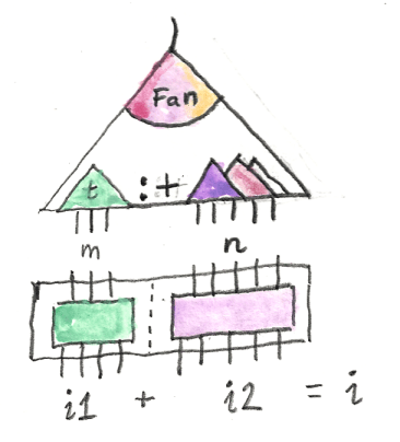
A MoveTree is either a Leaf with a nullary constructor, or a Fan, whose constructor takes Trees n:
data MoveTree n where
    Leaf ::               MoveTree One
    Fan  :: Trees n    -> MoveTree n
Trees is defined as an empty list NilT, or a cons of a branch consisting of a Move and a MoveTree followed by a tail of Trees:
data Trees n where
    NilT ::                                  Trees Z
    (:+) :: (Move, MoveTree k) -> Trees m -> Trees (k + m)

infixr 5 :+
You may recognize this data structure as an edge-labeled version of a rose tree. Here are a few examples of MoveTrees.
t1 :: MoveTree One
t1 = Leaf

t2 :: MoveTree Z
t2 = Fan (NilT)

t3 :: MoveTree One
t3 = Fan $ (Move Cross (FinS FinZ) FinZ, Leaf) :+ NilT

t4 :: MoveTree Two
t4 = Fan $ (Move Circle FinZ FinZ, t3)
        :+ (Move Circle FinZ (FinS FinZ), t3)
        :+ NilT
The last tree describes two possible branches: A circle at (0, 0) followed by a cross at (1, 0); and a circle at (0, 1) followed by a cross at (1, 0).

The compile-time parameter n in MoveTree n counts the number of leaves.
Of special interest is the infix constructor (:+) which has to add up the number of leaves in all branches. Here, the addition (k + m) must be performed on types rather than values. To define addition on types we use a multi-parameter type family — type family serving as a compile-time equivalent of a function. Here, the function is an infix operator (+). It takes two types of the kind Nat and produces a type of the kind Nat:
type family (+) (a :: Nat) (b :: Nat) :: Nat
The implementation of this compile-time function is defined inductively through two families of type instances. The base case covers the addition of zero on the left:
type instance Z + m = m
(This is an instance for the type family (+) written in the infix notation.)
The inductive step takes care of adding a successor of n, also on the left:
type instance S n + m = S (n + m)
Notice that the compiler won’t be able to deduce from these definitions that, for instance, m + Z is the same as m. We’ll have to do something special when the need arises — when we are forced to add a zero on the right. Compile-time arithmetic is funny that way.
Operad
The nice thing about move trees is that they are composable. It’s this composability that allows them to be used to speculatively predict multiple futures of a game. Given a current game tree, we can extend it by all possible moves of the computer player, and then extend it by all possible countermoves of the human opponent, and so on. This kind of grafting of trees on top of trees is captured by the operad.
What we are going to do is to consider our move trees as arrows with one or more inputs. Here things might get a little confusing, because a natural interpretation of a move tree is that its input is the first move, the root of the tree; and the leaves are the outputs. But for the sake of the operad, we’ll reverse the meaning of input and output.
In Haskell, we define a category by specifying the hom-set as a type. Then we define the composition of morphisms and pick the identity morphisms. We’ll do a similar thing with the operad. The difference is that an arrow in an operad is parameterized by the number of inputs (leaves of the tree). Continuing with the theme of compile-time safety, we’ll make this parameterization at compile-time.
The analog of the identity arrow will have a single input.
But how do we compose arrows that have multiple inputs? To compose an arrow with n inputs we need something that has n outputs. We can’t get n outputs from a single arrow (for n greater than 1) so we need a whole forest of arrows (with apologies for mixed metaphors). Composition in an operad connects an arrow to a forest. This is the definition:
class (Graded f) => Operad (f :: Nat -> *) where
  ident :: f (S Z)
  compose :: f n -> Forest f m n -> f m
Here, f is a compile-time function from Nat to a regular type — in other words, a data type parameterized by Nat. The identity has one input. Composition takes an n-ary arrow and a forest with m inputs and n outputs. As usual, the obvious identity and associativity laws are assumed but not expressible in Haskell. I’ll define the forest in a moment, but first let’s talk about the additional constraint, Graded f.
Conceptually, a Graded data type provides a way to retrieve its grade — or the count for a counted data structure — at runtime. But why would we need runtime grade information? Wasn’t the whole idea to perform the counting at compile time? It turns out that our compile-time Nats are great at parameterizing data structures. Types of the Nat kind can be used as phantom types. But the same trick won’t work for parameterizing polymorphic functions — there’s no place to insert phantom types into definitions of functions. A function type reflects the types of its arguments and the return type. So if we want to pass a compile-time count to a function, we have to do it through a dummy argument.
For that purpose we need a family of types parameterized by compile-time natural numbers. This time, though, the types must be inhabited, because we need to pass values of those types to functions. These values don’t have to carry any runtime information — they are only used to carry the type. It’s enough that each type be inhabited by a single dummy value, just like it is with the unit type (). Such types are called singleton types. Here’s the definition of the singleton natural number:
data SNat n where
  SZ :: SNat Z
  SS :: SNat n -> SNat (S n)
You can use it to create a series of values:
sZero :: SNat Z
sZero = SZ

sOne :: SNat One
sOne = SS SZ

sTwo :: SNst Two
sTwo = SS (SS SZ)
and so on…
You can also define a function for adding such values. It’s a polymorphic function that takes two singletons and produces another singleton. It really performs addition on types, but it gets the types at compile time from its arguments, and produces a singleton value of the correct type.
plus :: SNat n -> SNat m -> SNat (n + m)
plus SZ n = n
plus (SS n) m = SS (n `plus` m)
The Graded typeclass is defined for counted types — types that are parameterized by Nats:
class Graded (f :: Nat -> *) where
  grade :: f n -> SNat n
Our MoveTrees are easily graded:
instance Graded MoveTree where
    grade Leaf = SS SZ
    grade (Fan ts) = grade ts

instance Graded Trees where
    grade NilT = SZ
    grade ((_, t) :+ ts) = grade t `plus` grade ts
With those preliminaries out of the way, we are ready to implement the Operad instance for the MoveTree. We pick the single leaf tree as our identity.
ident = Leaf
Before we define composition, we have to define a forest. It’s a list of trees parameterized by two compile-time integers, which count the total number of inputs and outputs. A single tree f (our multi-input arrow) is parameterized by the number of inputs. It has the kind Nat->*.
data Forest f n m where
  Nil  :: Forest f Z Z
  Cons :: f i1 -> Forest f i2 n -> Forest f (i1 + i2) (S n)
The Nil constructor creates an empty forest with zero inputs and zero outputs. The Cons constructor takes a tree with i1 inputs (and, implicitly, one output), and a forest with i2 inputs and n outputs. The result is a forest with i1+i2 inputs and n+1 outputs.

Composition in the operad has the following signature:
compose :: f n -> Forest f m n -> f m
It produces a tree by plugging the outputs of a forest in the inputs of a tree.

We’ll implement composition in multiple stages. First, we make sure that a single leaf is the left identity of our operad. The simplest case is when the right operand is a single-leaf forest :
compose Leaf (Cons Leaf Nil) = Leaf

A little complication arises when we want to compose the identity with a single-tree forest. Naively, we would like to write:
compose Leaf (Cons t Nil) = t

This should work, since the leaf has one input, and the single-tree forest has one output. Looking at the signature of compose, the compiler should be able to deduce that n in the definition of compose should be replaced by S Z. Let’s follow the arithmetic.
The forest is the result of Consing a tree with i1 inputs, and a Nil forest with Z inputs and Z outputs. By definition of Cons, the resulting forest has i1+Z inputs and S Z outputs. So the ns in compose match. The problem is with unifying the ms. The one from the forest is equal to i1+Z, and the one on the right hand side is i1. And herein lies the trouble: we are adding Z on the right of i1. As I mentioned before, the compiler has no idea that i1+Z is the same as i1. We’re stuck! The solution to this problem requires some cheating, as well as digging into the brave new world of constraint kinds.
Constraint Kinds
We want to tell the compiler that two types, n and (n + Z) are the same. Both types are of the kind Nat. Equality of types can be expressed as a constraint with the tilde between the two types:
n ~ (n + Z)
Constraints are inhabitants of a special kind called Constraint. Besides type equality, they can express typeclass constraints like Eq or Num.
The compiler treats constraints as if they were types and, in fact, lets you define type aliases for them:
type Stringy a = (Show a, Read a)
Here, Stringy, just like Show and Read, is of the kind * -> Constraint. Unlike regular types of kind *, constraints are not inhabited by values. You can use them as contexts in front of the double arrow, =>, but you can’t pass them as runtime values.
This situation is very similar to what we’ve seen with the Nat kind, which also contained uninhabited types. But with Nat we were able to reify those types by defining the corresponding singletons. A very similar trick works with Constraints. A reified constraint singleton is called a Dict:
data Dict :: Constraint -> * where
  Dict :: a => Dict a
In particular, if a is a typeclass constraint, you can think of Dict as a class dictionary — the generalization of a virtual table. There is in fact a hidden singleton that is passed by the compiler to functions with typeclass constraints. For instance, the function:
print :: Show a => a -> IO ()
is translated to a function of two variables, one of them being the virtual table for the typeclass Show. When you call print with an Int, the compiler finds the virtual table for the Show instance of Int and passes it to print.
The difference is that now we are trying to do explicitly what the compiler normally hides from us.
Notice that Dict has only one constructor that takes no arguments. You can construct a Dict from thin air. But because it’s a polymorphic value, you either have to specify what type of Dict you want to construct, or give the compiler enough information to figure it out on its own.
How do you specify the concrete type of a Dict? Dict is a type constructor of the kind Constraint->* so, to define a specific type, you need to provide a constraint. For instance, you could construct a dictionary using the constraint that the type One is the same as the type (One + Z):
myDict :: Dict (One ~ (One + Z))
myDict = Dict
This actually works, but it doesn’t generalize. What we really need is a whole family of singletons parameterized by n:
plusZ :: forall n. Dict (n ~ (n + Z))
But the compiler is not able to verify an infinite family of constraints. We are stuck!
When everything else fails, try cheating. Cheating in Haskell is called unsafeCoerce. We can take a dictionary that we know exists, for instance that of (n ~ n) and force the compiler to believe that it’s the right type:
plusZ :: forall n. Dict (n ~ (n + Z))
plusZ = unsafeCoerce (Dict :: Dict (n ~ n))
This is to be expected: We are hitting the limits of Haskell. Haskell is not a dependent type language and it’s not a theorem prover. It’s possible to avoid some of the ugliness by using TypeLits, but I wanted to show you the low level details.
To truly understand the meaning of constraints, we should take a moment to talk about the Curry-Howard isomorphism. It tells us that types are equivalent to propositions: logical statement that can be either true or false. A type that is inhabited corresponds to a true statement. Most data types we define in a program are clearly inhabited. They have constructors that let us create values — the inhabitants of a given type. Then there are function types, which may or may not be inhabited. If you can implement a function of a given type, then you have a proof that this type is inhabited. Things get really interesting when you consider polymorphic functions. They correspond to propositions with quantifiers. We know, for instance, that the type a->a is inhabited for all a — we have the proof: the identity function.
A type like Dict is even more interesting. It explicitly specifies the condition under which it is inhabited. The type Dict a is inhabited if the constraint a is true. For instance, (n ~ n) is true, so the corresponding dictionary, Dict (n ~ n), can be constructed. What’s even more interesting is that, if you can hand the compiler an instance of a particular dictionary, it is proof enough that the constraint it encapsulates is true. The actual value of plusZ is irrelevant but its existence is critical.
So how do we bring it to the compiler’s attention? One way is to pass the dictionary as an argument to a function, but that’s awkward. In our case, the signature of the function compose is fixed. A better option is to bring a proof to the local scope by pattern matching.
compose Leaf (Cons (t :: MoveTree m) Nil) =
    case plusZ :: Dict (m ~ (m + Z)) of Dict -> t
Notice how we first introduce m into the scope by explicitly typing t inside the pattern for Forest. We fix the type of t to be:
MoveTree m
Then we explicitly type the value of plusZ, our global singleton, to be:
Dict (m ~ (m + Z))
This lets the compiler unify the n in the original definition of plusZ with our local m. Finally we pattern-match plusZ to its constructor, Dict. Obviously, the match will succeed. We don’t care about the result of this match, except that it introduces the proof of (m ~ (m + Z)) into the inner scope. It will let the compiler complete the type checking by unifying the actual type of t with the expected return type of compose.
Splitting the Forest
So far we have dealt with the simple cases of operadic composition, the ones where the left hand side had just one input. The general case involves connecting a tree that has k inputs to a forest that has k outputs and an arbitrary number of inputs. A MoveTree that is not a single Leaf is a Fan of Trees, which can be further split into the head tree and the tail. This corresponds to the pattern:
compose (Fan ((mv, t) :+ ts)) frt

We will proceed by recursion. The base case is the empty Fan:
compose (Fan NilT) Nil = Fan NilT
In the recursive case we have to split the forest frt into the part that matches the inputs of the tree t, and the remainder. The number of inputs of t is given by its grade — that’s why we needed the operad to be Graded.
If Forest was a simple list of trees, splitting it would be trivial: there’s even a function called splitAt in the Prelude. The fact that a Forest is counted makes it more interesting. But the real problem is that a Forest is parameterized by both the number of inputs and outputs. We want to separate a certain number of outputs, say m, but we have no idea how many inputs, i1, will go with that number of outputs. It depends on how much the individual trees branch inside the forest.
To see the problem, let’s try to come up with a signature for splitForest. It should look something like this:
splitForest :: SNat m -> SNat n -> Forest f i (m + n)
    -> (Forest f i1 m, Forest f i2 n)
But what are i1 and i2? All we know is that they exist and that they should add up to i. If there was an existential quantifier in Haskell, we could try writing something like this:
splitForest :: exists i1 i2. (i1 + i2 ~ i) =>
    SNat m -> SNat n -> Forest f i (m + n)
    -> (Forest f i1 m, Forest f i2 n)
We can’t do exactly that, but this pseudocode suggests a neat workaround. The existential quantifier may be replaced by a universal quantifier under a CPS transformation. There is a Curry-Howard reason for that, which has to do with CPS representing logical negation. But this can also be easily explained programmatically. Since we cannot predict how the inputs will split in the general case; instead of returning a concrete result we may ask the caller to provide a function — a continuation — that can accept an arbitrary split and take over from there. The continuation itself must be universally quantified: it must work for all splits. Here’s the signature of the continuation:
(forall i1 i2. (i ~ (i1 + i2)) =>
        (Forest f i1 m, Forest f i2 n) -> r)
As usual, when doing a CPS transform we don’t care what the type r is — in fact, we have to universally quantify over it. And since we have a local constraint that involves i, we have to bring i into the inner scope. The way to scope type variables in Haskell is to explicitly quantify over them. And once you quantify over one type variable, you have to quantify over all of them. That’s why the declaration of splitForest starts with one giant quantifier:
forall m n i f r
Putting it all together, here’s the final type signature of splitForest:
splitForest :: forall m n i f r. SNat m -> SNat n -> Forest f i (m+n)
    -> (forall i1 i2. (i ~ (i1 + i2)) =>
        (Forest f i1 m, Forest f i2 n) -> r)
    -> r
We will implement splitForest using recursion. The base case splits the forest at offset zero. It simply calls the continuation k with a pair consisting of an empty fragment and the unchanged forest:
splitForest SZ _ fs k = k (Nil, fs)
The recursive case is conceptually simple. The offset at which you split the forest is the successor of some number represented by a singleton sm. The forest itself is a Cons of a tree t and some tail ts. We want to split this tail into two fragments at sm — one less than (SS sm). We return the pair whose first component is the Cons of the tree t and the first fragment, and whose second component is the second fragment. Except that, instead of returning, we call the continuation. And in order to split the tail, we have to create another continuation to accept the fragments. So here’s the skeleton of the implementation:
splitForest (SS sm)
            sn
            (Cons t ts)
            k =
    splitForest sm sn ts $
        ((m_frag, n_frag) -> k (Cons t m_frag, n_frag)
To make this compile, we need to fill in some of the type signatures. In particular, we need to extract the number of inputs i1 and i2 from the constituents of the forest. We also have to extract the number of inputs i3 and i4 of the fragments. Finally, we have to tell the compiler that addition is associative. I won’t go into the gory details, I’ll just show you the final implementation:
splitForest (SS (sm :: SNat m_1))
            sn
            (Cons (t :: f i1) (ts :: Forest f i2 (m_1 + n)))
            k =
    splitForest sm sn ts $
        ((m_frag :: Forest f i3 m_1), (n_frag :: Forest f i4 n)) ->
            case plusAssoc (Proxy :: Proxy i1)
                           (Proxy :: Proxy i3)
                           (Proxy :: Proxy i4) of
               Dict -> k (Cons t m_frag, n_frag)
But what’s this Proxy business? The compiler is having — again — a problem with simple arithmetic. This time it’s the associativity of addition. We have to provide a proof that:
((i1 + i3) + i4) ~ (i1 + (i3 + i4))
But this time we can’t fake it with a polymorphic value; like we did with plusZ, which was parameterized by a single type of the kind Nat. We have to fake it with a polymorphic function:
plusAssoc :: p a -> q b -> r c -> Dict (((a + b) + c) ~ (a + (b + c)))
plusAssoc _ _ _ = unsafeCoerce (Dict :: Dict (a ~ a))
Here p, q, and r, are some arbitrary type constructors of the kind Nat->*. It doesn’t matter what the values of the arguements are, as long as they introduce the three (uninhabited) types, a, b, and c, into the scope. Proxy is a very simple polymorphic singleton type:
data Proxy t = Proxy
We create three Proxy values and call the function plusAssoc, which returns a dictionary that witnesses the associativity of the addition of the three Nats.
Equipped with the function splitForest, we can now complete our Operad instance:
instance Operad MoveTree where
    ident = Leaf
    compose Leaf (Cons Leaf Nil) = Leaf
    compose Leaf (Cons (t :: MoveTree m) Nil) =
        case plusZ :: Dict (m ~ (m + Z)) of Dict -> t
    compose (Fan NilT) Nil = Fan NilT
    compose (Fan ((mv, t) :+ ts)) frt =
        Fan $ splitForest (grade t) (grade ts) frt $
              (mts1, mts2) ->
                 let tree  = (compose t mts1)
                     (Fan trees) = (compose (Fan ts) mts2)
                 in (mv, tree) :+ trees
    compose _ _ = error "compose!"
The Comonad
A comonad is the dual of a monad. Just like a monad lets you lift a value using return, a comonad lets you extract a value. And just like a monad lets you collapse double encapsulation to single encapsulation using join, a comonad lets you duplicate the encapsulation.
class Functor w => Comonad w where
   extract :: w a -> a
   duplicate :: w a -> w (w a)
In other words, a monad lets you put stuff in and reduce whereas a comonad lets you take stuff out and reproduce.
A list monad, for instance, implements return by constructing a singleton list, and join by concatenating a list of lists.
An infinite list, or a stream comonad, implements extract by accessing the head of the list and duplicate by creating a stream of consecutive tails.
An operad can be used to define both a monad and a comonad. The monad M combines an operadic tree of n inputs with a vector of n elements.
data M f a where
   M :: f n -> Vec n a -> M f a
Monadic return combines the operadic identity with a singleton vector, whereas join grafts the operadic trees stored in the vector into the operad using compose and then concatenates the vectors.
The comonad W is also pretty straightforward. It’s defined as a polymorphic function, the evaluator, that takes an operad f n and produces a vector Vec n:
newtype W f a = W { runW :: forall n. f n -> Vec n a }

It’s obviously a functor:
instance Functor (W f) where
    fmap g (W k) = W $ f -> fmap g (k f)
Comonadic extract calls the evaluator with the identity operad and extracts the value from the singleton vector:
extract (W k) = case k ident of
    VCons a VNil -> a

The implementation of duplicate is a bit more involved. Its signature is:
duplicate :: W f -> W (W f)
Given the evaluator inside W f:
ev :: forall n. f n -> Vec n a
it has to produce another evaluator:
forall m. f m -> Vec m (W f)
This function, when called with an operadic tree f m, which I’ll call the outer tree, must produce m new evaluators.

What should the kth such evaluator do when called with the inner tree fi? The obvious thing is to graft the inner tree at the kth input of the outer tree. We can saturate the rest of the inputs of the outer tree with identities. Then we’ll call the evaluator ev with this new larger tree to get a larger vector. Our desired result will be in the middle of this vector at offset k.
This is the complete implementation of the comonad:
instance Operad f => Comonad (W f) where
  extract (W k) = case k ident of
    VCons a VNil -> a
  duplicate (W ev :: W f a) = W $ f -> go f SZ (grade f)
    where
      -- n increases, m decreases
      -- n starts at zero, m starts at (grade f)
      go :: f (n + m) -> SNat n -> SNat m -> Vec m (W f a)
      go _ _ SZ = VNil
      go f n (SS m) =  case succAssoc n m of
          Dict -> W ev' `VCons` go f (SS n) m
        where
          ev' :: f k -> Vec k a
          ev' fk = middleV n (grade fk) m
                           (ev (f `compose` plantTreeAt n m fk))
As usual, we had to help the compiler with the arithmetic. This time it was the associativity of the successor:
succAssoc :: p a -> q b -> Dict ((a + S b) ~ S (a + b))
succAssoc _ _ = unsafeCoerce (Dict :: Dict (a ~ a))
Notice that we didn’t have to use the Proxy trick in succAssoc n m, since we had the singletons handy.
The Tic Tac Toe Comonad
The W comonad works with any operad, in particular it will work with our MoveTree.
type TicTacToe = W MoveTree Evaluation
We want the evaluator for this comonad to produce a vector of Evaluations, which we will define as:
type Evaluation = (Score, MoveTree One)
The scoring is done from the perspective of the computer. A Bad move is a move that falls on an already marked square. A Good move carries with it an integer score:
data Score = Bad | Win | Lose | Good Int
  deriving (Show, Eq)
Evaluation includes a single-branch MoveTree One, which is the list of moves that led to this evaluation. In particular, the singleton Evaluation returned by extract will contain the history of moves up to the current point in the game.
Let’s see what duplicate does in our case. It produces a vector of TicTacToe games, each containing a new evaluator. These new evaluators, when called with a move tree, whether it’s a single move, a tree of 9 possible moves, a tree of 81 possible moves and responses, etc.; will graft this tree to the corresponding leaf of the previous game tree and perform the evaluation. We’ll call duplicate after every move and pick one of the resulting games (evaluators).
The Evaluator
This blog post is mostly about operads and comonads, so I won’t go into a lot of detail about implementing game strategy. I’ll just give a general overview, and if you’re curious, you can view the code on github.
The heart of the operadic comonad is the evaluator function. To start the whole process running, we’ll create the initial board. We’ll use the function eval that takes a board and returns an evaluator (which is eval partially applied to the board).
main :: IO ()
main = do
    putStrLn "Make your moves by entering x y coordinates 1..3 1..3."
    let board = emptyBoard
        game = W (eval board)
    play board game
The evaluator is a function that takes a MoveTree and returns a vector of Evaluation. If the tree is just a single leaf (that’s the identity of our operad), the evaluation is trivial. The interesting part is the evaluation of a Fan of branches.
eval :: Board -> MoveTree n -> Vec n Evaluation
eval board moves = case moves of
    Leaf   -> singleV (Good 0, Leaf)
    Fan ts -> evalTs (evalBranch board) ts
The function evalTs iterates over branches, applying a branch evaluator to each tree and concatenating the resulting evaluation vectors. The only tricky part is that each branch may end in a different number of leaves, so the branch evaluator must be polymorphic in k:
evalTs :: (forall k. (Move, MoveTree k) -> Vec k Evaluation)
          -> Trees n
          -> Vec n Evaluation
evalTs _ NilT = VNil
evalTs ev (br :+ ts) = concatV (ev br) (evalTs f ts)
The branch evaluator must account for the possibility that a move might be invalid — it has to test whether the square has already been marked on the board. If it’s not, it marks the board and evaluates the move.
First, there are two simple cases: the move could be a winning move or a losing move. In those cases when the result is known immediately, that is Bad, Win, or Lose, evalBranch returns a vector of the size determined by the number of leaves in the branch. The vector is filled with the appropriate values (Bad, Win, or Lose).
The interesting case is when the move is neither invalid nor decisive. In that case we recurse into eval with the new board and the sub-tree that follows the move in question. We gather the resulting evaluations and adjust the scores. If any of the branches results in a loss, we lower the score on all of them. Otherwise we add the score of the current move to all scores for that tree.
Game Logic
At the very top level we have the game loop, which takes input from the user and responds with the computer’s move. A user move must be tested for correctness. First it’s converted to two Fin Three values (or Nothing). Then we create a singleton MoveTree with that move and pass it to the evaluator. If the move is invalid, we continue prompting the user. If the move is decisive, we announce the winner. Otherwise, we advance the game by calling duplicate, and then pick the new evaluator from the resulting tree of comonadic values — the one corresponding to the user move.
To generate the computer response, we create a two-deep tree of all possible moves (that is one computer move and one user move — that seems to be enough of the depth to win or tie every time). We call the evaluator with that tree and pick the best result. Again, if it’s a decisive move, we announce the winner. Otherwise, we call duplicate again, and pick the new evaluator corresponding to the selected move.
Conclusion
Does it make sense to implement tic-tac-toe using such heavy machinery? Not really! But it makes sense as an exercise in compile-time safety guarantees. I wouldn’t mind if those techniques were applied to writing software that makes life-and-death decisions. Nuclear reactors, killer drones, or airplane auto-pilots come to mind. Fast stock-trading software, even though it cannot kill you directly, can also be mission critical, if you’re attached to your billions. What’s an overkill in one situation may save your life in another. You need different tools for different tasks and Haskell provides the options.
The full source is available on github.
Thanks go to André van Meulebrouck for his editing help.