You may think of Tannakian Reconstruction as an example of redundant encoding. It lets you replace a simple hom-set with a much more complex end that is taken over an entire functor category.

Why would anyone want to do it? The answer is simple: composition! Morphisms on the left compose according to the rules of the category 

Optics
A simple category of optics over a single category 


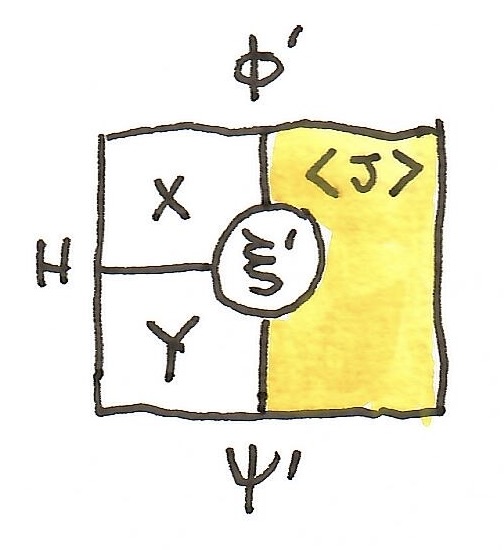
In what follows, we’ll be using the fact that an element of a coend can be constructed by injecting a triple 


Optics compose by “zooming in”:

The identity optic is given by injecting the triple 

where:

is the left unitor for the monoidal action and 
The archetypical optic is a lens, whose action is defined as the cartesian product in

In Haskell, we would encode it as an existential type:
data Lens s t a b = forall m . Lens (s -> (m, a)) ((m, b) -> t)
This formula can be expanded using the mapping-in property of the product (or, in an alternative derivation, its mapping out property, that is currying):

Using the Yoneda reduction (a.k.a. “integrating” over 

which, in Haskell, corresponds to a pair of functions:
get :: s -> aset :: s -> b -> t
The getter extracts the subobject a, the focus of the lens. The setter replaces it with b.
Lenses compose by zooming in: the focus of one lens becomes the source of the other.

In Haskell this can be encoded as:
composeLens :: Lens a b a' b' -> Lens s t a b -> Lens s t a' b'composeLens (Lens l2 r2) (Lens l1 r1) = Lens l3 r3 where l3 = assoc' . second l2 . l1 r3 = r1 . second r2 . assoc assoc ((c, c'), b') = (c, (c', b')) assoc' (c, (c', a')) = ((c, c'), a')
As you can see, optic composition can be quite messy. That’s where the Tannakian representation saves the day.
Optics and Tambara modules
The idea is to follow the Tannakian reconstruction by defining the category of set-valued functors over the category of optics and use the end over these functors to represent optics.
It turns out that set-valued functors on optics are our old friends, Tambara modules. There is an equivalence of categories:
![[\mathbf{Opt}^{op}, Set] \cong \mathbf{Tamb}](https://s0.wp.com/latex.php?latex=%5B%5Cmathbf%7BOpt%7D%5E%7Bop%7D%2C+Set%5D+%5Ccong+%5Cmathbf%7BTamb%7D&bg=ffffff&fg=29303b&s=0&c=20201002)
We use the opposite category of optics because, traditionally, optic composition is defiened in terms of zooming in rather than zooming out. Thus the slogan is: Presheaves on optics are Tambara modules.
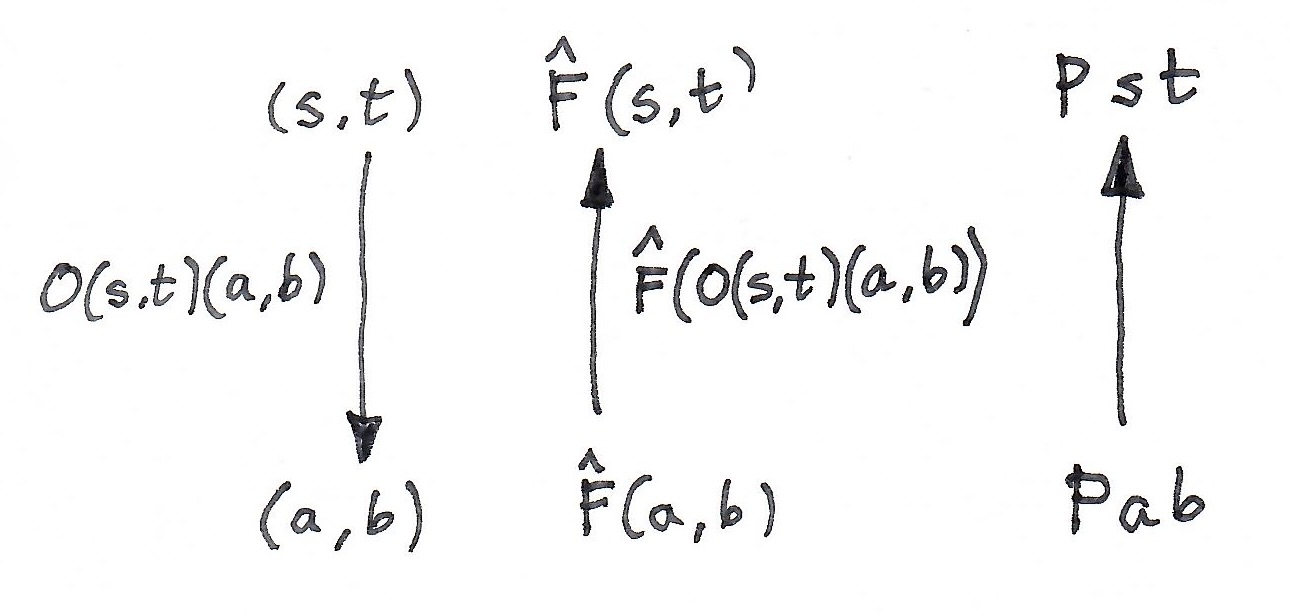
Let’s first analyze the definition of a presheaf ![\hat F \in [\mathbf{Opt}^{op}, Set]](https://s0.wp.com/latex.php?latex=%5Chat+F+%5Cin+%5B%5Cmathbf%7BOpt%7D%5E%7Bop%7D%2C+Set%5D&bg=ffffff&fg=29303b&s=0&c=20201002)

On morphisms, it maps optics to functions (reversing the direction). Thus an optic:
is mapped to a function:

The plan is to construct two mappings: from presheaves to Tambara modules and another from Tambara modules to presheaves. They have to be defined on (pairs of) objects as well as on morphisms. I will first sketch the proof using category theory and then translate it, step by step, to Haskell.
From presheaf to Tambara
On objects, given a presheaf 

We know that it’s a profunctor because, given a pair of morphisms:


we can construct a mapping:

We do this by lifting an optic of the type:

This optic can be instantiated by injecting 
The tricky part is to equip 

In this case, we want to implement:

We’ll do this by lifting a carefuly chosen optic of the type:

This optic is given by the following coend:

We instantiate it by injecting the triple 
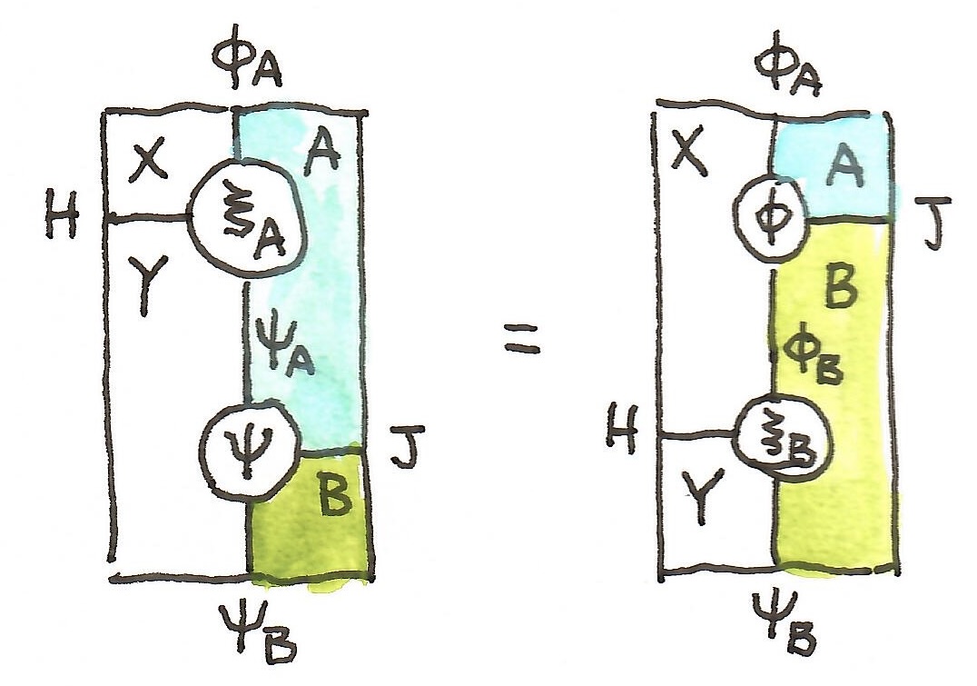
On morphisms, we want to map an optic to an element of the hom-set 

Using the co-continuity of the hom-set, we replace the mapping out of a coend with the end:

We have at our disposal a pair of morphisms:
which, together with the Tambara structure, give us the desired mapping:

From Tambara to presheaf
On objects, given a Tambara module

On morphisms, we have to map a function on Tambara modules 
An optic 


We want to produce:

We have at our disposal a pair of morphisms:


We know that simple hom-sets are Tambara modules, so we can apply the Tambara structure to both morphism:


After re-associating the iterated actions we inject the triple that consist of 
Profunctor representation of optics
Since presheaves on 

This is the general form of the profunctor representation of optics that works for any monoidal action.
Haskell implementation
In Haskell, we can encode general optics (morphisms in
data Opt ten act1 act2 s t a b = forall m. (Actegory ten act1, Actegory ten act2) => Opt (s -> m `act1` a) (m `act2` b -> t)
Notice that it’s okay to use two different actions (in fact, one can use two different categories). The corresponding Tambara modules are defined as:
class (Actegory ten act1, Actegory ten act2, Profunctor p) => Tambara ten act1 act2 p where leftAct :: p a b -> p (m `act1` a) (m `act2` b)
The profunctor representation of these optics is given by a polymorphic function type:
type TamRep ten act1 act2 s t a b = forall p . (Tambara ten act1 act2 p) => p a b -> p s t
Such functions can be composed (optics, zoomed in) using simple function composition.
Proof of equivalence
To prove the equivalence of the two representation, we need some additional definitions.
Here’s the unit optic that uses the unitors:
unitOpt :: (Actegory ten act1, Actegory ten act2) => Opt ten act1 act2 a b a bunitOpt = Opt unit' unit
Since we are working with the oposite category, we define the flipped version of optics:
data FlipOpt ten act1 act2 a b s t = FlipOpt (Opt ten act1 act2 s t a b)
FlipOpt is an instance of Tambara:
instance (Actegory ten act1, Actegory ten act2) => Tambara ten act1 act2 (FlipOpt ten act1 act2 a b) where leftAct (FlipOpt (Opt l r)) = FlipOpt (Opt l' r') -- take advantage of the Tambara structure on hom-sets -- l :: s -> m a, l' :: n s -> n m a -- r :: m b -> t, r' :: n m b -> n t where l' = assoc' . leftAct @ten @act1 @act1 @(->) l r' = leftAct @ten @act2 @act2 @(->) r . assoc
I made the use of the Tambara action on hom-functors explicit through type annotations.
Here’s the mapping from optics to the Tambara representation:
toProRep :: (Actegory ten act1, Actegory ten act2) => Opt ten act1 act2 s t a b -> TamRep ten act1 act2 s t a btoProRep (Opt s_ma mb_t) pab = dimap s_ma mb_t (leftAct pab)
The opposite mapping uses the flipped unit optics. This is why we needed the proof that flipped optic is a Tambara module. As such, we can pass it to our function that is polymorphic in Tambara modules:
fromProRep :: (Actegory ten act1, Actegory ten act2) => TamRep ten act1 act2 s t a b -> Opt ten act1 act2 s t a bfromProRep pab_pst = opt where FlipOpt opt = pab_pst (FlipOpt unitOpt)
Examples
By plugging in different monoidal categories and their actions, we can immediately generate Tambara representations for a variety of optics.
We can use the Tambara encoding for the lens:
type Lens s t a b = forall p . Tambara (,) (,) (,) p => p a b -> p s t
Here’s the example of a prism:
data Prism s t a b = forall m . Prism (s -> Either m a) (Either m b -> t)
and its Tambara representation:
type Prism' s t a b = forall p . Tambara Either Either Either p => p a b -> p s t
Haskell code for this post is available here.
![[C, Set]](https://s0.wp.com/latex.php?latex=%5BC%2C+Set%5D&bg=ffffff&fg=29303b&s=0&c=20201002) (for historical reasons, these are called co-presheaves). Such a functor maps objects to sets, and morphisms to functions.
(for historical reasons, these are called co-presheaves). Such a functor maps objects to sets, and morphisms to functions.  we will associate a mapping from functors to sets, simply by applying each functor to this object
  :
:![\Phi_c \colon [C, Set] \to Set](https://s0.wp.com/latex.php?latex=%5CPhi_c+%5Ccolon+%5BC%2C+Set%5D+%5Cto+Set&bg=ffffff&fg=29303b&s=0&c=20201002)

 is a family of functions
  . We define the action of
  on a natural transformation by taking its component
  .
. is called a fiber functor. You may think of it as probing an object and, through morphisms, its immediate neighborhood.
  we’ll be looking at the set of functions
  under all possible functors
  .
. , a hom-set in the functor category:
![[[C, Set], Set] (\Phi_a, \Phi_b)](https://s0.wp.com/latex.php?latex=%5B%5BC%2C+Set%5D%2C+Set%5D+%28%5CPhi_a%2C+%5CPhi_b%29&bg=ffffff&fg=29303b&s=0&c=20201002)
![\int_{\hat F \colon [C, Set]} Set (\Phi_a \hat F, \Phi_b \hat F) = \int_{\hat F \colon [C, Set]} Set (\hat F a, \hat F b)](https://s0.wp.com/latex.php?latex=%5Cint_%7B%5Chat+F+%5Ccolon+%5BC%2C+Set%5D%7D+Set+%28%5CPhi_a+%5Chat+F%2C+%5CPhi_b+%5Chat+F%29+%3D+%5Cint_%7B%5Chat+F+%5Ccolon+%5BC%2C+Set%5D%7D+Set+%28%5Chat+F+a%2C+%5Chat+F+b%29&bg=ffffff&fg=29303b&s=0&c=20201002)
 and empty at
  ? Such a single bad apple would spoil the whole batch (there is no function from a non-empty set to an empty set).
 , we automatically have a function
![[C, Set] (C(a, -), \hat F) \cong \hat F a](https://s0.wp.com/latex.php?latex=%5BC%2C+Set%5D+%28C%28a%2C+-%29%2C+%5Chat+F%29+%5Ccong+%5Chat+F+a&bg=ffffff&fg=29303b&s=0&c=20201002)
![\int_{\hat F} Set ([C, Set] (C(a,-), \hat F), [C, Set] (C(b, -), \hat F)](https://s0.wp.com/latex.php?latex=%5Cint_%7B%5Chat+F%7D+Set+%28%5BC%2C+Set%5D+%28C%28a%2C-%29%2C+%5Chat+F%29%2C+%5BC%2C+Set%5D+%28C%28b%2C+-%29%2C+%5Chat+F%29&bg=ffffff&fg=29303b&s=0&c=20201002)
![[C, Set] (C(b, -), C(a, -))](https://s0.wp.com/latex.php?latex=%5BC%2C+Set%5D+%28C%28b%2C+-%29%2C+C%28a%2C+-%29%29&bg=ffffff&fg=29303b&s=0&c=20201002)
 equipped with the transformation:


 , where actegories are 0-cells, Tambara modules with coend composition are 1-cells, and natural transformations between them are 2-cells.
 in which categories are 0-cells, profunctors are horizontal arrows, functors are vertical arrows, and natural transformations form 2-cells. This double category happens to be a
  as the profunctor:
 . In Haskell this is:

 to the lifting of
 to
to  (it forgets the action). This functor has a left adjoint. For any profunctor
 . Indeed, applying the Yoneda reduction, we get:
![\mathbf M \to [C, C]](https://s0.wp.com/latex.php?latex=%5Cmathbf+M+%5Cto+%5BC%2C+C%5D&bg=ffffff&fg=29303b&s=0&c=20201002) , can be internalized in
, can be internalized in  if it has a right adjoint:


![\int^{c \colon [\mathbb N , Set]} C(s, \sum_n c_n \times a^n) \times C (\sum_m c_m \times b^m, t)](https://s0.wp.com/latex.php?latex=%5Cint%5E%7Bc+%5Ccolon+%5B%5Cmathbb+N+%2C+Set%5D%7D+C%28s%2C+%5Csum_n+c_n+%5Ctimes+a%5En%29+%5Ctimes+C+%28%5Csum_m+c_m+%5Ctimes+b%5Em%2C+t%29&bg=ffffff&fg=29303b&s=0&c=20201002)
 and
and  are powers.

 is automatically a monoid in

 . We assume that this product is associative and unital– up to isomorphism. It means that there is an invertible associator:


![\triangleright \colon \mathbf M \to [C, C]](https://s0.wp.com/latex.php?latex=%5Ctriangleright+%5Ccolon+%5Cmathbf+M+%5Cto+%5BC%2C+C%5D&bg=ffffff&fg=29303b&s=0&c=20201002)
 to the tensor product
  and its unit

 as the monoidal category.)

 arrow, replacing it with its horizontal conjoint
  . In a profunctor equipment, this is just a representable profunctor
  .
. 
 of the shape below can be uniquely factorized through the counit
  :
:


 along a horizontal 1-cell


 and in
  . In Haskell, we can define them as two types:
 , the comma category
  consists of pairs
  . In other words, it’s a category of arrows from the image of
  to some fixed object
  . Morphisms in the comma category are arrows
  in
in  that make the corresponding triangles in
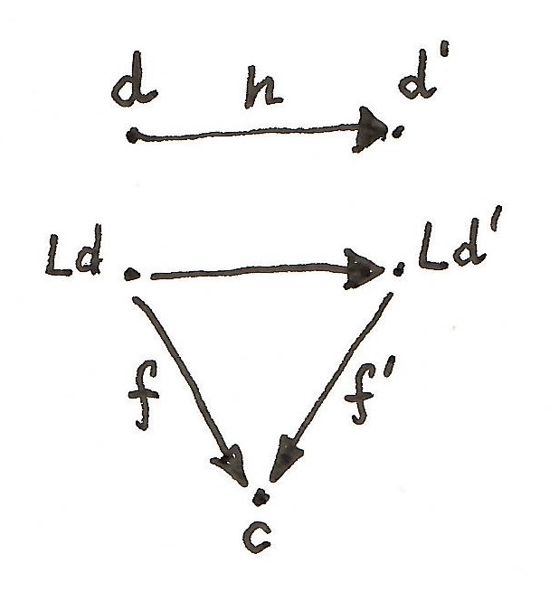
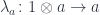
 , through which every arrow
  factorizes uniquely. That means, there is a unique arrow
  that makes the following triangle commute:
 , then we can easily construct the universal arrow as a pair
  , where
  is a component of the counit of the adjunction. Indeed, every
 .
.

 , where
  is functor precomposition. Or as a string diagram:


 . Similarly, a graph of a relation is a set of pairs where
  . If the set is empty, it means that the objects are unrelated.
 , an object in the category of elements is a triple
  . We interpret
  as a witness that
  is a pair of morphisms
  such that:
 is the whiskering, or the lifting of a pair of morphisms, one of which is an identity, by the profunctor
  . We want the result, in both cases, to give us the same element of
  — the witness that
  .
.
 is a 0-cell
  equipped with two projections. Think of these projections as extracting the two objects from the triple that we used in the definition of a graph of a profunctor. Their relation to
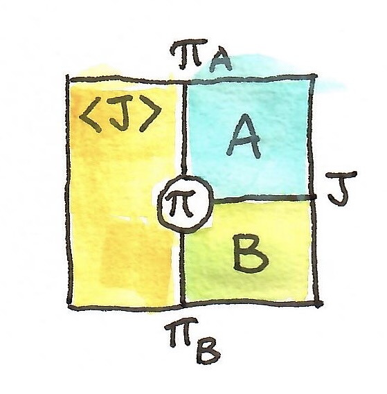

 is a natural transformation whose components are:
 and the result is an element of the set
  .
.  or
or  , both leading to the same result.
 . We postulate that for any 0-cell
  and
and  there is a unique factorization through the universal 2-cell
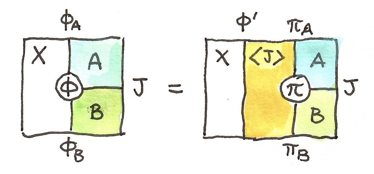


 , on objects, as:
 , as
, as  .
. . All we have to provide is two vertical arrows and a 2-cell. But to complete the picture, we should be able to construct a 2-cell from another horizontal 1-cell,
  together with a projection
  , such that:
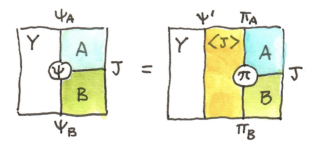


 :
:
 and
and  factor through it. Here’s the first factorization:
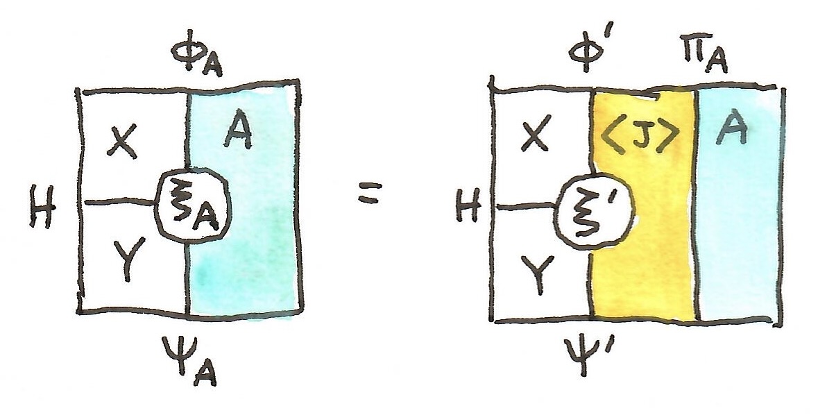

 , we get as the target a pair of morphisms:
 , we can construct such a pair as:
 this produces
  thus satisfying the 2-dimensional universal condition. The constraints on
  with
with  .
. that is somehow related to a vertical arrow
  . There are two 2-cells that illustrate this relation, but it’s not clear what their meaning is or how to use them.
 . Diagrammatically, we have:
 , is illustrated by the following diagrams:

 and
and  and turns them into
  and
and  . Then we shove the two counits below it (vertically postcompose), to bend the arrows
  and
and  .
.  and
and  , a cartesian square defines a horizontal arrow
  also called a restriction of
 . To this end we replace
  , together with two new vertical arrows
  and
and  that, just like
 over a pair of 1-cells
  , given the corresponding cartesian square
  .
.

 , with functors as morphisms.
 . In fact, profunctors can be considered arrows in the category
  . Not only that,
 is the identity profunctor with respect to this composition. It means that we have a way of talking about hom-sets and representables without peeking inside individual categories.
 with two (horizontal) profunctors
  and
and  .
. 
 is a function:

 is sometimes called the restriction of
  , in diagram order).


 with the appropriate injection into the coend.
 implementing the functoriality of
 , is defined in

 stands for comPanion):
 .
.
 is the identity at


 :
:


 . Or we can consider a simpler case of the double category of sets and relations. We can also add more structure to the categories in question, for instance by considering monoidal categories; or even go meta, and study the double category of (weak) double categories
  .
.