December 2021
Monthly Archive
December 28, 2021
A PDF version of this post is available on github.
Abstract
Co-presheaf optic is a new kind of optic that generalizes the polynomial lens. Its distinguishing feature is that it’s not based on the action of a monoidal category. Instead the action is parameterized by functors between different co-presheaves. The composition of these actions corresponds to composition of functors rather than the more traditional tensor product. These functors and their composition have a representation in terms of profunctors.
Motivation
A lot of optics can be defined using the existential, or coend, representation:

Here  is a monoidal category with an action on objects of two categories
  and
and  (I’ll use the same notation for both actions). The actions are composed using the tensor product in :

The idea of this optic is that we have a pair of morphisms, one decomposing the source  into the action of some
  on
on  , and the other recomposing the target
  from the action of the same on
  . In most applications we pick to be the same category as .
Recently, there has been renewed interest in polynomial functors. Morphisms between polynomial functors form a new kind of optic that doesn’t neatly fit this mold. They do, however, admit an existential representation or the form:

Here the sets  and
and  can be treated as fibers over the set
  , while the sets
  and
and  are fibers over a different set
  .
.
Alternatively, we can treat these fibrations as functors from discrete categories to  , that is co-presheaves. For instance is the result of a co-presheaf acting on an object
  of a discrete category
  . The products over can be interpreted as ends that define natural transformations between co-presheaves. The interesting part is that the matrices
  are fibrated over two different sets. I have previously interpreted them as profunctors:
In this post I will elaborate on this interpretation.
Co-presheaves
A co-presheaf category ![[\mathcal C, Set ]](https://s0.wp.com/latex.php?latex=%5B%5Cmathcal+C%2C+Set+%5D&bg=ffffff&fg=29303b&s=0&c=20201002) behaves, in many respects, like a vector space. For instance, it has a “basis” consisting of representable functors
behaves, in many respects, like a vector space. For instance, it has a “basis” consisting of representable functors  ; in the sense that any co-presheaf is as a colimit of representables. Moreover, colimit-preserving functors between co-presheaf categories are very similar to linear transformations between vector spaces. Of particular interest are functors that are left adjoint to some other functors, since left adjoints preserve colimits.
The polynomial lens formula has a form suggestive of vector-space interpretation. We have one vector space with vectors  and
and  and another with
  and
and  . Rectangular matrices can be seen as components of a linear transformation between these two vector spaces. We can, for instance, write:
where  is the transposed matrix. Transposition here serves as an analog of adjunction.
We can now re-cast the polynomial lens formula in terms of co-presheaves. We no longer intepret and  as discrete categories. We have:
![a, b \colon [\mathcal N, \mathbf{Set}]](https://s0.wp.com/latex.php?latex=a%2C+b+%5Ccolon+%5B%5Cmathcal+N%2C+%5Cmathbf%7BSet%7D%5D+&bg=ffffff&fg=29303b&s=0&c=20201002)
![s, t \colon [\mathcal K, \mathbf{Set}]](https://s0.wp.com/latex.php?latex=s%2C+t+%5Ccolon+%5B%5Cmathcal+K%2C+%5Cmathbf%7BSet%7D%5D+&bg=ffffff&fg=29303b&s=0&c=20201002)
In this interpretation  is a functor between categories of co-presheaves:
![c \colon [\mathcal N, \mathbf{Set}] \to [\mathcal K, \mathbf{Set}]](https://s0.wp.com/latex.php?latex=c+%5Ccolon+%5B%5Cmathcal+N%2C+%5Cmathbf%7BSet%7D%5D+%5Cto+%5B%5Cmathcal+K%2C+%5Cmathbf%7BSet%7D%5D+&bg=ffffff&fg=29303b&s=0&c=20201002)
We’ll write the action of this functor on a presheaf as  .
.
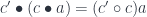
We assume that this functor has a right adjoint and therefore preserves colimits.
![[\mathcal K, \mathbf{Set}] (c \bullet a, t) \cong [\mathcal N, \mathbf{Set}] (a, c^{\dagger} \bullet t)](https://s0.wp.com/latex.php?latex=%5B%5Cmathcal+K%2C+%5Cmathbf%7BSet%7D%5D+%28c+%5Cbullet+a%2C+t%29+%5Ccong+%5B%5Cmathcal+N%2C+%5Cmathbf%7BSet%7D%5D+%28a%2C+c%5E%7B%5Cdagger%7D+%5Cbullet+t%29+&bg=ffffff&fg=29303b&s=0&c=20201002)
where:
![c^{\dagger} \colon [\mathcal K, \mathbf{Set}] \to [\mathcal N, \mathbf{Set}]](https://s0.wp.com/latex.php?latex=c%5E%7B%5Cdagger%7D+%5Ccolon+%5B%5Cmathcal+K%2C+%5Cmathbf%7BSet%7D%5D+%5Cto+%5B%5Cmathcal+N%2C+%5Cmathbf%7BSet%7D%5D+&bg=ffffff&fg=29303b&s=0&c=20201002)
We can now generalize the polynomial optic formula to:
![\mathcal{O}\langle a, b\rangle \langle s, t \rangle = \int^{c} [\mathcal K, \mathbf{Set}] \left(s, c \bullet a \right) \times [\mathcal K, \mathbf{Set}] \left(c \bullet b, t \right)](https://s0.wp.com/latex.php?latex=%5Cmathcal%7BO%7D%5Clangle+a%2C+b%5Crangle+%5Clangle+s%2C+t+%5Crangle+%3D+%5Cint%5E%7Bc%7D+%5B%5Cmathcal+K%2C+%5Cmathbf%7BSet%7D%5D+%5Cleft%28s%2C++c+%5Cbullet+a+%5Cright%29+%5Ctimes+%5B%5Cmathcal+K%2C+%5Cmathbf%7BSet%7D%5D+%5Cleft%28c+%5Cbullet+b%2C+t+%5Cright%29+&bg=ffffff&fg=29303b&s=0&c=20201002)
The coend is taken over all functors that have a right adjoint. Fortunately there is a better representation for such functors. It turns out that colimit preserving functors:
are equivalent to profunctors (see the Appendix for the proof). Such a profunctor:

is given by the formula:
where  is a representable co-presheaf.
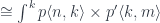
The action of can be expressed as a coend:
The co-presheaf optic is then a coend over all profunctors 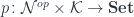 :
:
![\int^{p} [\mathcal K, \mathbf{Set}] \left(s, \int^{n} a(n) \times p \langle n, - \rangle \right) \times [\mathcal K, \mathbf{Set}] \left(\int^{n'} b(n') \times p \langle n', - \rangle, t \right)](https://s0.wp.com/latex.php?latex=%5Cint%5E%7Bp%7D+%5B%5Cmathcal+K%2C+%5Cmathbf%7BSet%7D%5D+%5Cleft%28s%2C++%5Cint%5E%7Bn%7D+a%28n%29+%5Ctimes+p+%5Clangle+n%2C+-+%5Crangle+%5Cright%29+%5Ctimes+%5B%5Cmathcal+K%2C+%5Cmathbf%7BSet%7D%5D+%5Cleft%28%5Cint%5E%7Bn%27%7D+b%28n%27%29+%5Ctimes+p+%5Clangle+n%27%2C+-+%5Crangle%2C+t+%5Cright%29+&bg=ffffff&fg=29303b&s=0&c=20201002)
Composition
We have defined the action as the action of a functor on a co-presheaf. Given two composable functors:
![c \colon [\mathcal N, \mathbf{Set}] \to [\mathcal K, \mathbf{Set}]](https://s0.wp.com/latex.php?latex=c+%5Ccolon++%5B%5Cmathcal+N%2C+%5Cmathbf%7BSet%7D%5D+%5Cto+%5B%5Cmathcal+K%2C+%5Cmathbf%7BSet%7D%5D+&bg=ffffff&fg=29303b&s=0&c=20201002)
and:
![c' \colon [\mathcal K, \mathbf{Set}] \to [\mathcal M, \mathbf{Set}]](https://s0.wp.com/latex.php?latex=c%27+%5Ccolon++%5B%5Cmathcal+K%2C+%5Cmathbf%7BSet%7D%5D+%5Cto+%5B%5Cmathcal+M%2C+%5Cmathbf%7BSet%7D%5D+&bg=ffffff&fg=29303b&s=0&c=20201002)
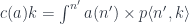
we automatically get the associativity law:
The composition of functors between co-presheaves translates directly to profunctor composition. Indeed, the profunctor  corresponding to
  is given by:

and can be evaluated to:

which is the standard definition of profunctor composition.
Consider two composable co-presheaf optics,  and
and  . The first one tells us that there exists a and a pair of natural transformations:
![l_c (s, a ) = [\mathcal K, \mathbf{Set}] \left(s, c \bullet a \right)](https://s0.wp.com/latex.php?latex=l_c+%28s%2C++a+%29+%3D+%5B%5Cmathcal+K%2C+%5Cmathbf%7BSet%7D%5D+%5Cleft%28s%2C++c+%5Cbullet+a+%5Cright%29+&bg=ffffff&fg=29303b&s=0&c=20201002)
![r_c (b, t) = [\mathcal K, \mathbf{Set}] \left(c \bullet b, t \right)](https://s0.wp.com/latex.php?latex=r_c+%28b%2C+t%29+%3D+%5B%5Cmathcal+K%2C+%5Cmathbf%7BSet%7D%5D+%5Cleft%28c+%5Cbullet+b%2C+t+%5Cright%29+&bg=ffffff&fg=29303b&s=0&c=20201002)
The second tells us that there exists a  and a pair:
![l'_{c'} (a, a' ) = [\mathcal K, \mathbf{Set}] \left(a, c' \bullet a' \right)](https://s0.wp.com/latex.php?latex=l%27_%7Bc%27%7D+%28a%2C++a%27+%29+%3D+%5B%5Cmathcal+K%2C+%5Cmathbf%7BSet%7D%5D+%5Cleft%28a%2C++c%27+%5Cbullet+a%27+%5Cright%29+&bg=ffffff&fg=29303b&s=0&c=20201002)
![r'_{c'} (b', b) = [\mathcal K, \mathbf{Set}] \left(c' \bullet b', b \right)](https://s0.wp.com/latex.php?latex=r%27_%7Bc%27%7D+%28b%27%2C+b%29+%3D+%5B%5Cmathcal+K%2C+%5Cmathbf%7BSet%7D%5D+%5Cleft%28c%27+%5Cbullet+b%27%2C+b+%5Cright%29+&bg=ffffff&fg=29303b&s=0&c=20201002)
The composition of the two should be an optic of the type  . Indeed, we can construct such an optic using the composition and a pair of natural transformations:


Generalizations
By duality, there is a corresponding optic based on presheaves. Also, (co-) presheaves can be naturally generalized to enriched categories, where the correspondence between left adjoint functors and enriched profunctors holds as well.
Appendix
I will show that a functor between two co-presheaves that has a right adjoint and therefore preserves colimits:
is equivalent to a profunctor:
The profunctor is given by:
and the functor can be recovered using the formula:
where:
![a \colon [\mathcal N, \mathbf{Set}]](https://s0.wp.com/latex.php?latex=a+%5Ccolon+%5B%5Cmathcal+N%2C+%5Cmathbf%7BSet%7D%5D+&bg=ffffff&fg=29303b&s=0&c=20201002)
I’ll show that these formulas are the inverse of each other. First, inserting the formula for into the definition of  should gives us back:

which follows from the co-Yoneda lemma.
Second, inserting the formula for into the definition of should give us back:
Since preserves all colimits, and any co-presheaf is a colimit of representables, it’s enough that we prove this identity for a representable:
We have to show that:

and this follows from the co-Yoneda lemma.
December 20, 2021
Posted by Bartosz Milewski under
Philosophy,
Physics
[6] Comments
From the outside it might seem like physics and mathematics are a match made in heaven. In practice, it feels more like physicists are given a very short blanket made of math, and when they stretch it to cover their heads, their feet are freezing, and vice versa.
Physicists turn reality into numbers. They process these numbers using mathematics, and turn them into predictions about other numbers. The mapping between physical reality and mathematical models is not at all straightforward. It involves a lot of arbitrary choices. When we perform an experiment, we take the readings of our instruments and create one particular parameterization of nature. There usually are many equivalent parameterizations of the same process and this is one of the sources of redundancy in our description of nature. The Universe doesn’t care about our choice of units or coordinate systems.
This indifference, after we plug the numbers into our models, is reflected in symmetries of our models. A change in the parameters of our measuring apparatus must be compensated by a transformation of our model, so that the results of calculations still match the outcome of the experiment.
But there is an even deeper source of symmetries in physics. The model itself may introduce additional redundancy in order to simplify the calculations or, sometimes, make them possible. It is often necessary to use parameter spaces that allow the description of non-physical states–states that could never occur in reality.
Computer programmers are familiar with such situations. For instance, we often use integers to access arrays. But an integer can be negative, or it can be larger than the size of the array. We could say that an integer can describe “non-physical” states of the array. We also have freedom of parameterization of our input data: we can encode true as one, and false as zero; or the other way around. If we change our parameterization, we must modify the code that deals with it. As programmers we are very well aware of the arbitrariness of the choice of representation, but it’s even more true in physics. In physics, these reparameterizations are much more extensive and they have their mathematical description as groups of transformations.
But what we see in physics is very strange: the non-physical degrees of freedom introduced through redundant parameterizations turn out to have some measurable consequences.
Symmetries
If you ask physicists what the foundations of physics are, they will probably say: symmetry. Depending on their area of research, they will start talking about various symmetry groups, like SU(3), U(1), SO(3,1), general diffeomorphisms, etc. The foundations of physics are built upon fields and their symmetries. For physicists this is such an obvious observation that they assume that the goal of physics is to discover the symmetries of nature. But are symmetries the property of nature, or are they the artifact of our tools? This is a difficult question, because the only way we can study nature is through the prism or mathematics. Mathematical models of reality definitely exhibit lots of symmetries, and it’s easy to confuse this with the statement that nature itself is symmetric.
But why would models exhibit symmetry? One explanation is that symmetries are the effect of redundant descriptions.
I’ll use the example of electromagnetism because of its relative simplicity (some of the notation is explained in the Appendix), but the redundant degrees of freedom and the symmetries they generate show up everywhere in physics. The Standard Model is one big gauge theory, and Einstein’s General Relativity is built on the principle of invariance with respect to local coordinate transformations.
Electromagnetic field
Maxwell’s equations are a mess, until you rewrite them using 4-dimensional spacetime. The two vector fields, the electric field and the magnetic field are combined into one 4-dimensional antisymmetric tensor  :
:

Because of antisymmetry, has only six independent components. The components of are physical fields that can be measured using test charges and magnetic needles.
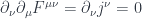
The derivatives of these fields satisfy two sets of Maxwell’s equations. The first set of four describes the dependence of fields on sources—electric charges and currents:

The second set of four equations describe constraints imposed on these fields:
![\partial_{[\rho} F_{\mu \nu ]} = 0](https://s0.wp.com/latex.php?latex=%5Cpartial_%7B%5B%5Crho%7D+F_%7B%5Cmu+%5Cnu+%5D%7D+%3D+0&bg=ffffff&fg=29303b&s=0&c=20201002)
For a particular set of sources and an initial configuration, we could try to solve these equations numerically. A brute force approach would be to divide space into little cubes, distribute our charges and currents between them, replace differential equations with difference equations, and turn on the crank.
First, we would check if the initial field configuration satisfied the constraints. Then we would calculate time derivatives of the fields. We would turn time derivatives into time differences by multiplying them by a small time period, get the next configuration, and so on. With the size of the cubes and the quantum of time small enough, we could get a reasonable approximation of reality. A program to perform these calculations isn’t much harder to write than a lot of modern 3-d computer games.
Notice that this procedure has an important property. To calculate the value of a field in a particular cube, it’s enough to know the values at its nearest neighbors and its value at the previous moment of time. The nearest-neighbor property is called locality and the dependence on the past, as opposed to the future, is called causality. The famous Conway Game of Life is local and causal, and so are cellular automata.
We were very lucky to be able to formulate a model that pretty well approximates reality and has these properties. Without such models, it would be extremely hard to calculate anything. Essentially all classical physics is written in the language of differential equations, which means it’s local, and its time dependence is carefully crafted to be causal. But it should be stressed that locality and causality are properties of particular models. And locality, in particular, cannot be taken for granted.
Electromagnetic Potential
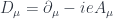
The second set of Maxwell’s equations can be solved by introducing a new field, a 4-vector  called the vector potential. The field tensor can be expressed as its anti-symmetrized derivative
![F_{\mu \nu} = \partial_{[ \mu} A_{\nu ]}](https://s0.wp.com/latex.php?latex=F_%7B%5Cmu+%5Cnu%7D+%3D+%5Cpartial_%7B%5B+%5Cmu%7D+A_%7B%5Cnu+%5D%7D&bg=ffffff&fg=29303b&s=0&c=20201002)
Indeed, if we take its partial derivative and antisymmetrize the three indices, we get:
![\partial_{[\rho} F_{\mu \nu ]} = \partial_{[\rho} \partial_{ \mu} A_{\nu ]} = 0](https://s0.wp.com/latex.php?latex=%5Cpartial_%7B%5B%5Crho%7D+F_%7B%5Cmu+%5Cnu+%5D%7D+%3D+%5Cpartial_%7B%5B%5Crho%7D+%5Cpartial_%7B+%5Cmu%7D+A_%7B%5Cnu+%5D%7D+%3D+0&bg=ffffff&fg=29303b&s=0&c=20201002)
which vanishes because derivatives are symmetric,  .
.
Note for mathematicians: Think of as a connection in the U(1) fiber bundle, and  as its curvature. The second Maxwell equation is the Bianchi identity for this connection.
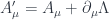
This field is not physical. We cannot measure it. We can measure its derivatives in the form of , but not the field itself. In fact we cannot distinguish between and the transformed field:
Here,  is a completely arbitrary, time dependent scalar field. This is, again, because of the symmetry of partial derivatives:
![F_{\mu \nu}' = \partial_{[ \mu} A'_{\nu ]} = \partial_{[ \mu} A_{\nu ]} + \partial_{[ \mu} \partial_{\nu ]} \Lambda = \partial_{[ \mu} A_{\nu ]} = F_{\mu \nu}](https://s0.wp.com/latex.php?latex=F_%7B%5Cmu+%5Cnu%7D%27+%3D+%5Cpartial_%7B%5B+%5Cmu%7D+A%27_%7B%5Cnu+%5D%7D+%3D+%5Cpartial_%7B%5B+%5Cmu%7D+A_%7B%5Cnu+%5D%7D+%2B+%5Cpartial_%7B%5B+%5Cmu%7D+%5Cpartial_%7B%5Cnu+%5D%7D+%5CLambda+%3D+%5Cpartial_%7B%5B+%5Cmu%7D+A_%7B%5Cnu+%5D%7D+%3D+F_%7B%5Cmu+%5Cnu%7D&bg=ffffff&fg=29303b&s=0&c=20201002)
Adding a derivative of  is called a gauge transformation, and we can formulated a new law: Physics in invariant under gauge transformations. There is a beautiful symmetry we have discovered in nature.
But wait a moment: didn’t we just introduce this symmetry to simplify the math?
Well, it’s a bit more complicated. To explain that, we have to dive even deeper into technicalities.
The Action Principle
You cannot change the past and your cannot immediately influence far away events. These are the reasons why differential equations are so useful in physics. But there are some types of phenomena that are easier to explain by global rather than local reasoning. For instance, if you span an elastic rubber band between two points in space, it will trace a straight line. In this case, instead of diligently solving differential equations that describe the movements of the rubber band, we can guess its final state by calculating the shortest path between two points.
Surprisingly, just like the shape of the rubber band can be calculated by minimizing the length of the curve it spans, so the evolution of all classical systems can be calculated by minimizing (or, more precisely, finding a stationary point of) a quantity called the action. For mechanical systems the action is the integral of the Lagrangian along the trajectory, and the Lagrangian is given by the difference between kinetic and potential energy.
Consider the simple example of an object thrown into the air and falling down due to gravity. Instead of solving the differential equations that relate acceleration to force, we can reformulate the problem in terms of minimizing the action. There is a tradeoff: we want to minimize the kinetic energy while maximizing the potential energy. Potential energy is larger at higher altitudes, so the object wants to get as high as possible in the shortest time, stay there as long as possible, before returning to earth. But the faster it tries to get there, the higher its kinetic energy. So it performs a balancing act resulting is a perfect parabola (at least if we ignore air resistance).
The same principle can be applied to fields, except that the action is now given by a 4-dimensional integral over spacetime of something called the Lagrangian density which, at every point, depends only of fields and their derivatives. This is the classical Lagrangian density that describes the electromagnetic field:
and the action is:

However, if you want to derive Maxwell’s equations using the action principle, you have to express it in terms of the potential and its derivatives.
Noether’s Theorem
The first of the Maxwell’s equations describes the relationship between electromagnetic fields and the rest of the world:
Here “the rest of the world” is summarized in a 4-dimensional current density  . This is all the information about matter that the fields need to know. In fact, this equation imposes additional constraints on the matter. If you differentiate it once more, you get:
Again, this follows from the antisymmetry of and the symmetry of partial derivatives.
The equation:

is called the conservation of electric charge. In terms of 3-d components it reads:

or, in words, the change in charge density is equal to the divergence of the electric current. Globally, it means that charge cannot appear or disappear. If your isolated system starts with a certain charge, it will end up with the same charge.
Why would the presence of electromagnetic fields impose conditions on the behavior of matter? Surprisingly, this too follows from gauge invariance. Electromagnetic fields must interact with matter in a way that makes it impossible to detect the non-physical vector potentials. In other words, the interaction must be gauge invariant. Which makes the whole action, which combines the pure-field Lagrangian and the interaction Lagrangian, gauge invariant.
It turns out that any time you have such an invariance of the action, you automatically get a conserved quantity. This is called the Noether’s theorem and, in the case of electromagnetic theory, it justifies the conservation of charge. So, even though the potentials are not physical, their symmetry has a very physical consequence: the conservation of charge.
Quantum Electrodynamics
The original idea of quantum field theory (QFT) was that it should extend the classical theory. It should be able to explain all the classical behavior plus quantum deviations from it.
This is no longer true. We don’t insist on extending classical behavior any more. We use QFT to, for instance, describe quarks, for which there is no classical theory.
The starting point of any QFT is still the good old Lagrangian density. But in quantum theory, instead of minimizing the action, we also consider quantum fluctuations around the stationary points. In fact, we consider all possible paths. It just so happens that the contributions from those paths that are far away from the classical solutions tend to cancel each other. This is the reason why classical physics works so well: classical trajectories are the most probable ones.
In quantum theory, we calculate probabilities of transitions from the initial state to the final state. These probabilities are given by summing up complex amplitudes for every possible path and then taking the absolute value of the result. The amplitudes are given by the exponential of the action:

Far away from the stationary point of the action, the amplitudes corresponding to adjacent paths vary very quickly in phase and they cancel each other. The summation effectively acts like a low-pass filter for these amplitudes. We are observing the Universe through a low-pass filter.
In quantum electrodynamics things are a little tricky. We would like to consider all possible paths in terms of the vector potential  . The problem is that two such paths that differ only by a gauge transformation result in exactly the same action, since the Lagrangian is written in terms of gauge invariant fields . The action is therefore constant along gauge transformations and the sum over all such paths would result in infinity. Once again, the non-physical nature of the potential raises its ugly head.
Another way of describing the same problem is that we expect the quantization of electromagnetic field to describe the quanta of such field, namely photons. But a photon has only two degrees of freedom corresponding to two polarizations, whereas a vector potential has four components. Besides the two physical ones, it also introduces longitudinal and time-like polarizations, which are not present in the real world.
To eliminate the non-physical degrees of freedom, physicists came up with lots of clever tricks. These tricks are relatively mild in the case of QED, but when it comes to non-Abelian gauge fields, the details are quite gory and involve the introduction of even more non-physical fields called ghosts.
Still, there is no way of getting away from vector potentials. Moreover, the interaction of the electromagnetic field with charged particles can only be described using potentials. For instance, the Lagrangian for the electron field  in the electromagnetic field is:
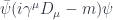
The potential is hidden inside the covariant derivative
where  is the electron charge.
Note for mathematicians: The covariant derivative locally describes parallel transport in the U(1) bundle.
The electron is described by a complex Dirac spinor field . Just as the electromagnetic potential is non-physical, so are the components of the electron field. You can conceptualize it as a “square root” of a physical field. Square roots of numbers come in pairs, positive and negative—Dirac field describes both negative electrons and positive positrons. In general, square roots are complex, and so are Dirac fields. Even the field equation they satisfy behaves like a square root of the conventional Klein-Gordon equation. Most importantly, Dirac field is only defined up to a complex phase. You can multiply it by a complex number of modulus one,  (the in the exponent is the charge of the electron). Because the Lagrangian pairs the field with its complex conjugate
  , the phases cancel, which shows that the Lagrangian does not depend on the choice of the phase.
In fact, the phase can vary from point to point (and time to time) as long as the phase change is compensated by the the corresponding gauge transformation of the electromagnetic potential. The whole Lagrangian is invariant under the following simultaneous gauge transformations of all fields:


The important part is the cancellation between the derivative of the transformed field and the gauge transformation of the potential:

Note for mathematicians: Dirac field forms a representation of the U(1) group.
Since the electron filed is coupled to the potential, does it mean that an electron can be used to detect the potential? But the potential is non-physical: it’s only defined up to a gauge transformation.
The answer is really strange. Locally, the potential is not measurable, but it may have some very interesting global effects. This is one of these situations where quantum mechanics defies locality. We may have a region of space where the electromagnetic field is zero but the potential is not. Such potential must, at least locally, be of the form:  . Such potential is called pure gauge, because it can be “gauged away” using
  .
.
But in a topologically nontrivial space, it may be possible to define a pure-gauge potential that cannot be gauged away by a continuous function. For instance, if we remove a narrow infinite cylinder from a 3-d space, the rest has a non-trivial topology (there are loops that cannot be shrunk to a point). We could define a 3-d vector potential that circulates around the cylinder. For any fixed radius around the cylinder, the field would consist of constant-length vectors that are tangent to the circle. A constant function is a derivative of a linear function, so this potential could be gauged away using a function that linearly increases with the angle around the cylinder, like a spiral staircase. But once we make a full circle, we end up on a different floor. There is no continuous that would eliminate this potential.
This is not just a theoretical possibility. The field around a very long thin solenoid has this property. It’s all concentrated inside the solenoid and (almost) zero outside, yet its vector potential cannot be eliminated using a continuous gauge transformation.
Classically, there is no way to detect this kind of potential. But if you look at it from the perspective of an electron trying to pass by, the potential is higher on one side of the solenoid and lower on the other, and that means the phase of the electron field will be different, depending whether it passes on the left, or on the right of it. The phase itself is not measurable but, in quantum theory, the same electron can take both paths simultaneously and interfere with itself. The phase difference is translated into the shift in the interference pattern. This is called the Aharonov-Bohm effect and it has been confirmed experimentally.
Note for mathematicians: Here, the base space of the fiber bundle has non-trivial homotopy. There may be non-trivial connections that have zero curvature.

Aharonov-Bohm experiment
Space Pasta
I went into some detail to describe the role redundant degrees of freedom and their associated symmetries play in the theory of electromagnetic fields.
We know that the vector potentials are not physical: we have no way of measuring them directly. We know that in quantum mechanics they describe non-existent particles like longitudinal and time-like photons. Since we use redundant parameterization of fields, we introduce seemingly artificial symmetries.
And yet, these “bogus symmetries” have some physical consequences: they explain the conservation of charge; and the “bogus degrees of freedom” explain the results of the Aharonov-Bohm experiment. There are some parts of reality that they capture. What are these parts?
One possible answer is that we introduce redundant parametrizations in order to describe, locally, the phenomena of global or topological nature. This is pretty obvious in the case of the Aharonov-Bohm experiment where we create a topologically nontrivial space in which some paths are not shrinkable. The charge conservation case is subtler.
Consider the path a charged particle carves in space-time. If you remove this path, you get a topologically non-trivial space. Charge conservation makes this path unbreakable, so you can view it as defining a topological invariant of the surrounding space. I would even argue that charge quantization (all charges are multiples of 1/3 of the charge or the electron) can be explained this way. We know that topological invariants, like the Euler characteristic that describes the genus of a manifold, take whole-number values.
We’d like physics to describe the whole Universe but we know that current theories fail in some areas. For instance, they cannot tell us what happens at the center of a black hole or at the Big Bang singularity. These places are far away, either in space or in time, so we don’t worry about them too much. There’s still a lot of Universe left for physicist to explore.
Except that there are some unexplorable places right under our noses. Every elementary particle is surrounded by a very tiny bubble that’s unavailable to physics. When we try to extrapolate our current theories to smaller and smaller distances, we eventually hit the wall. Our calculations result in infinities. Some of these infinities can be swept under the rug using clever tricks like renormalization. But when we get close to Planck’s distance, the effects of gravity take over, and renormalization breaks down.
So if we wanted to define “physical space” as the place where physics is applicable, we’d have to exclude all the tiny volumes around the paths of elementary particles. Removing the spaghetti of all such paths leaves us with a topological mess. This is the mess on which we define all our theories. The redundant descriptions and symmetries are our way of probing the excluded spaces.
Appendix
A point in Minkowski spacetime is characterized by four coordinates 
 , where
  is the time coordinate, and the rest are space coordinates. We use the system of units in which the speed of light is one.
Repeated indices are, by Einstein convention, summed over (contracted). Indices between square brackets are anisymmetrized (that is summed over all permutations, with the minus sign for odd permutations). For instance
![F_{0 1} = \partial_{[0} A_{1]} = \partial_{0} A_{1} - \partial_{1} A_{0} = \partial_{t} A_{x} - \partial_{x} A_{t}](https://s0.wp.com/latex.php?latex=F_%7B0+1%7D+%3D+%5Cpartial_%7B%5B0%7D+A_%7B1%5D%7D+%3D+%5Cpartial_%7B0%7D+A_%7B1%7D+-+%5Cpartial_%7B1%7D+A_%7B0%7D+%3D+%5Cpartial_%7Bt%7D+A_%7Bx%7D+-+%5Cpartial_%7Bx%7D+A_%7Bt%7D&bg=ffffff&fg=29303b&s=0&c=20201002)
Indexes are raised and lowered by contracting them with the Minkowski metric tensor:

Partial derivatives with respect to these coordinates are written as:

4-dimensional antisymmetric tensor is a  matrix, but because of antisymmetry, it reduces to just 6 independent entries, which can be rearranged into two 3-d vector fields. The vector
  is the electric field, and the vector
  is the magnetic field.

The sources of these fields are described by a 4-dimensional vector  . Its zeroth component describes the distribution of electric charges, and the rest describes electric current density.
The second set of Maxwell’s equations can also be written using the completely antisymmetric Levi-Civita tensor with entries equal to 1 or -1 depending on the parity of the permutation of the indices:
December 10, 2021
A PDF of this post is available on github.
Motivation
In this post I’ll be looking at a subcategory of  that consists of polynomial functors in which the fibration is done over one fixed set :

The reason for this restriction is that morphisms between such functors, which are called polynomial lenses, can be understood in terms of monoidal actions. Optics that have this property automatically have profunctor representation. Profunctor representation has the advantage that it lets us compose optics using regular function composition.
Previously I’ve explored the representations of polynomial lenses as optics in terms on functors and profunctors on discrete categories. With just a few modifications, we can make these categories non-discrete. The trick is to replace sums with coends and products with ends; and, when appropriate, interpret ends as natural transformations.
Monoidal Action
Here’s the existential representation of a lens between polynomials in which all fibrations are over the same set :


This makes the matrices “square.” Such matrices can be multiplied using a version of matrix multiplication.
Interestingly, this idea generalizes naturally to a setting in which is replaced by a non-discrete category  . In this setting, we’ll write the residues
  as profunctors:

They are objects in the monoidal category in which the tensor product is given by profunctor composition:

and the unit is the hom-functor  . (Incidentally, a monoid in this category is called a promonad.)
In the case of a discrete category, these definitions decay to standard matrix multiplication:

and the Kronecker delta  .
.
We define the monoidal action of the profunctor acting on a co-presheaf as:
This is reminiscent of a vector being multiplied by a matrix. Such an action of a monoidal category equips the co-presheaf category with the structure of an actegory.
A product of hom-sets in the definition of the existential optic turns into a set of natural transformations in the functor category ![[\mathcal{N}, \mathbf{Set}]](https://s0.wp.com/latex.php?latex=%5B%5Cmathcal%7BN%7D%2C+%5Cmathbf%7BSet%7D%5D+&bg=ffffff&fg=29303b&s=0&c=20201002) .
.
![\mathbf{Pl}\langle s, t\rangle \langle a, b\rangle \cong \int^{c \colon [\mathcal{N}^{op} \times \mathcal{N}, Set]} [\mathcal{N}, \mathbf{Set}] \left(s, c \bullet a\right) \times [\mathcal{N}, \mathbf{Set}] \left(c \bullet b, t\right)](https://s0.wp.com/latex.php?latex=%5Cmathbf%7BPl%7D%5Clangle+s%2C+t%5Crangle+%5Clangle+a%2C+b%5Crangle+%5Ccong+%5Cint%5E%7Bc+%5Ccolon+%5B%5Cmathcal%7BN%7D%5E%7Bop%7D+%5Ctimes+%5Cmathcal%7BN%7D%2C+Set%5D%7D+++%5B%5Cmathcal%7BN%7D%2C+%5Cmathbf%7BSet%7D%5D++%5Cleft%28s%2C+c+%5Cbullet+a%5Cright%29++%5Ctimes++%5B%5Cmathcal%7BN%7D%2C+%5Cmathbf%7BSet%7D%5D++%5Cleft%28c+%5Cbullet+b%2C+t%5Cright%29+&bg=ffffff&fg=29303b&s=0&c=20201002)
Or, using the end notation for natural transformations:

As before, we can eliminate the coend if we can isolate in the second hom-set using a series of isomorphisms:

![\cong \int_{n, k} \mathbf{Set}\left(c\langle k, n \rangle , [b(k), t (n)]\right)](https://s0.wp.com/latex.php?latex=%5Ccong+++%5Cint_%7Bn%2C+k%7D+%5Cmathbf%7BSet%7D%5Cleft%28c%5Clangle+k%2C+n+%5Crangle+%2C+%5Bb%28k%29%2C+t+%28n%29%5D%5Cright%29+&bg=ffffff&fg=29303b&s=0&c=20201002)
I used the fact that a mapping out of a coend is an end. The result, after applying the Yoneda lemma to eliminate the end over  , is:
, is:
![\mathbf{Pl}\langle s, t\rangle \langle a, b\rangle \cong \int_m \mathbf{Set}\left(s(m), \int^j a(j) \times [b(j), t(m)] \right)](https://s0.wp.com/latex.php?latex=%5Cmathbf%7BPl%7D%5Clangle+s%2C+t%5Crangle+%5Clangle+a%2C+b%5Crangle+%5Ccong+%5Cint_m+%5Cmathbf%7BSet%7D%5Cleft%28s%28m%29%2C+%5Cint%5Ej+a%28j%29+%5Ctimes+%5Bb%28j%29%2C+t%28m%29%5D+%5Cright%29&bg=ffffff&fg=29303b&s=0&c=20201002)
or, with some abuse of notation:
![[\mathcal{N}, \mathbf{Set}] ( s, [b, t] \bullet a)](https://s0.wp.com/latex.php?latex=%5B%5Cmathcal%7BN%7D%2C+%5Cmathbf%7BSet%7D%5D+%28+s%2C+%5Bb%2C+t%5D+%5Cbullet+a%29&bg=ffffff&fg=29303b&s=0&c=20201002)
When is discrete, this formula decays to the one for polynomial lens.
Profunctor Representation
Since this poly-lens is a special case of a general optic, it automatically has a profunctor representation. The trick is to define a generalized Tambara module, that is a category  of profunctors of the type:
![P \colon [\mathcal{N}, \mathbf{Set}]^{op} \times [\mathcal{N}, \mathbf{Set}] \to \mathbf{Set}](https://s0.wp.com/latex.php?latex=P+%5Ccolon+%5B%5Cmathcal%7BN%7D%2C+%5Cmathbf%7BSet%7D%5D%5E%7Bop%7D++%5Ctimes+%5B%5Cmathcal%7BN%7D%2C+%5Cmathbf%7BSet%7D%5D+%5Cto+%5Cmathbf%7BSet%7D+&bg=ffffff&fg=29303b&s=0&c=20201002)
with additional structure given by the following family of transformations, in components:

The profunctor representation of the polynomial lens is then given by an end over all profunctors in this Tambara category:

Where  is the obvious forgetful functor from to the underlying profunctor category$.
December 9, 2021
Lenses and, more general, optics are an example of hard-core category theory that has immediate application in programming. While working on polynomial lenses, I had a vague idea how they could be implemented in a programming language. I thought up an example of a polynomial lens that would focus on all the leaves of a tree at once. It could retrieve or modify them in a single operation. There already is a Haskell optic called traversal that could do it. It can safely retrieve a list of leaves from a tree. But there is a slight problem when it comes to replacing them: the size of the input list has to match the number of leaves in the tree. If it doesn’t, the traversal doesn’t work.
A polynomial lens adds an additional layer of safety by keeping track of the sizes of both the trees and the lists. The problem is that its implementation requires dependent types. Haskell has some support for dependent types, so I tried to work with it, but I quickly got bogged down. So I decided to bite the bullet and quickly learn Idris. This was actually easier than I expected and this post is the result.
Counted Vectors and Trees
I started with the “Hello World!” of dependent types: counted vectors. Notice that, in Idris, type signatures use a single colon rather than the Haskell’s double colon. You can quickly get used to it after the compiler slaps you a few times.
data Vect : Type -> Nat -> Type where
  VNil : Vect a Z
  VCons : (x: a) -> (xs : Vect a n) -> Vect a (S n)
If you know Haskell GADTs, you can easily read this definition. In Haskell, we usually think of Nat as a “kind”, but in Idris types and values live in the same space. Nat is just an implementation of Peano artithmetics, with Z standing for zero, and (S n) for the successor of n. Here, VNil is the constructor of an empty vector of size Z, and VCons prepends a value of type a to the tail of size n resulting in a new vector of size (S n). Notice that Idris is much more explicit about types than Haskell.
The power of dependent types is in very strict type checking of both the implementation and of usage of functions. For instance, when mapping a function over a vector, we can make sure that the result is the same size as the argument:
mapV : (a -> b) -> Vect a n -> Vect b n
mapV f VNil = VNil
mapV f (VCons a v) = VCons (f a) (mapV f v)
When concatenating two vectors, the length of the result must be the sum of the two lengths, (plus m n):
concatV : Vect a m -> Vect a n -> Vect a (plus m n)
concatV VNil v = v
concatV (VCons a w) v = VCons a (concatV w v)
Similarly, when splitting a vector in two, the lengths must match, too:
splitV : (n : Nat) -> Vect a (plus n m) -> (Vect a n, Vect a m)
splitV Z v = (VNil, v)
splitV (S k) (VCons a v') = let (v1, v2) = splitV k v'
                            in (VCons a v1, v2)
Here’s a more complex piece of code that implements insertion sort:
sortV : Ord a => Vect a n -> Vect a n
sortV VNil = VNil
sortV (VCons x xs) = let xsrt = sortV xs
                     in (ins x xsrt)
  where
    ins : Ord a => (x : a) -> (xsrt : Vect a n) -> Vect a (S n)
    ins x VNil = VCons x VNil
    ins x (VCons y xs) = if x < y then VCons x (VCons y xs)
                                  else VCons y (ins x xs)
In preparation for the polynomial lens example, let’s implement a node-counted binary tree. Notice that we are counting nodes, not leaves. That’s why the node count for Node is the sum of the node counts of the children plus one:
data Tree : Type -> Nat -> Type where
  Empty : Tree a Z
  Leaf  : a -> Tree a (S Z)
  Node  : Tree a n -> Tree a m -> Tree a (S (plus m  n))
All this is not much different from what you’d see in a Haskell library.
Existential Types
So far we’ve been dealing with function that return vectors whose lengths can be easily calculated from the inputs and verified at compile time. This is not always possible, though. In particular, we are interested in retrieving a vector of leaves from a tree that’s parameterized by the number of nodes. We don’t know up front how many leaves a given tree might have. Enter existential types.
An existential type hides part of its implementation. An existential vector, for instance, hides its size. The receiver of an existential vector knows that the size “exists”, but its value is inaccessible. You might wonder then: What can be done with such a mystery vector? The only way for the client to deal with it is to provide a function that is insensitive to the size of the hidden vector. A function that is polymorphic in the size of its argument. Our sortV is an example of such a function.
Here’s the definition of an existential vector:
data SomeVect : Type -> Type where
  HideV : {n : Nat} -> Vect a n -> SomeVect a
SomeVect is a type constructor that depends on the type a—the payload of the vector. The data constructor HideV takes two arguments, but the first one is surrounded by a pair of braces. This is called an implicit argument. The compiler will figure out its value from the type of the second argument, which is Vect a n. Here’s how you construct an existential:
secretV : SomeVect Int
secretV = HideV (VCons 42 VNil)
In this case, the compiler will deduce n to be equal to one, but the recipient of secretV will have no way of figuring this out.
Since we’ll be using types parameterized by Nat a lot, let’s define a type synonym:
Nt : Type
Nt = Nat -> Type
Both Vect a and Tree a are examples of this type.
We can also define a generic existential for stashing such types:
data Some : Nt -> Type where
  Hide : {n : Nat} -> nt n -> Some nt
and some handy type synonyms:
SomeVect : Type -> Type
SomeVect a = Some (Vect a)
SomeTree : Type -> Type
SomeTree a = Some (Tree a)
Polynomial Lens
We want to translate the following categorical definition of a polynomial lens:
![\mathbf{PolyLens}\langle s, t\rangle \langle a, b\rangle = \prod_{k} \mathbf{Set}\left(s_k, \sum_{n} a_n \times [b_n, t_k] \right)](https://s0.wp.com/latex.php?latex=%5Cmathbf%7BPolyLens%7D%5Clangle+s%2C+t%5Crangle+%5Clangle+a%2C+b%5Crangle+%3D+%5Cprod_%7Bk%7D+%5Cmathbf%7BSet%7D%5Cleft%28s_k%2C+%5Csum_%7Bn%7D+a_n+%5Ctimes+%5Bb_n%2C+t_k%5D+%5Cright%29+&bg=ffffff&fg=29303b&s=0&c=20201002)
We’ll do it step by step. First of all, we’ll assume, for simplicity, that the indices and are natural numbers. Therefore the four arguments to PolyLens are types parameterized by Nat, for which we have a type alias:
PolyLens : Nt -> Nt -> Nt -> Nt -> Type
The definition starts with a big product over all ‘s. Such a product corresponds, in programming, to a polymorphic function. In Haskell we would write it as forall k. In Idris, we’ll accomplish the same using an implicit argument {k : Nat}.
The hom-set notation  stands for a set of functions from to , or the type
 a -> b. So does the notation ![[a, b]](https://s0.wp.com/latex.php?latex=%5Ba%2C+b%5D&bg=ffffff&fg=29303b&s=0&c=20201002) (the internal hom is the same as the external hom in ). The product
(the internal hom is the same as the external hom in ). The product  is the type of pairs
 (a, b).
The only tricky part is the sum over . A sum corresponds exactly to an existential type. Our SomeVect, for instance, can be considered a sum over n of all vector types Vect a n.
Here’s the intuition: Consider that to construct a sum type like Either a b it’s enough to provide a value of either type a or type b. Once the Either is constructed, the information about which one was used is lost. If you want to use an Either, you have to provide two functions, one for each of the two branches of the case statement. Similarly, to construct SomeVect its enough to provide a vector of some particular lenght n. Instead of having two possibilities of Either, we have infinitely many possibilities corresponding to different n‘s. The information about what n was used is then promptly lost.
The sum in the definition of the polynomial lens:
![\sum_{n} a_n \times [b_n, t_k]](https://s0.wp.com/latex.php?latex=%5Csum_%7Bn%7D+a_n+%5Ctimes+%5Bb_n%2C+t_k%5D+&bg=ffffff&fg=29303b&s=0&c=20201002)
can be encoded in this existential type:
data SomePair : Nt -> Nt -> Nt -> Type where
  HidePair : {n : Nat} ->
             (k : Nat) -> a n -> (b n -> t k) -> SomePair a b t
Notice that we are hiding n, but not k.
Taking it all together, we end up with the following type definition:
PolyLens : Nt -> Nt -> Nt -> Nt -> Type
PolyLens s t a b = {k : Nat} -> s k -> SomePair a b t
The way we read this definition is that PolyLens is a function polymorphic in k. Given a value of the type s k it produces and existential pair SomePair a b t. This pair contains a value of the type a n and a function b n -> t k. The important part is that the value of n is hidden from the caller inside the existential type.
Using the Lens
Because of the existential type, it’s not immediately obvious how one can use the polynomial lens. For instance, we would like to be able to extract the foci a n, but we don’t know what the value of n is. The trick is to hide n inside an existential Some. Here is the “getter” for this lens:
getLens :  PolyLens sn tn an bn -> sn n -> Some an
getLens lens t =
  let  HidePair k v _ = lens t
  in Hide v
We call lens with the argument t, pattern match on the constructor HidePair and immediately hide the contents back using the constructor Hide. The compiler is smart enough to know that the existential value of n hasn’t been leaked.
The second component of SomePair, the “setter”, is trickier to use because, without knowing the value of n, we don’t know what argument to pass to it. The trick is to take advantage of the match between the producer and the consumer that are the two components of the existential pair. Without disclosing the value of n we can take the a‘s and use a polymorphic function to transform them into b‘s.
transLens : PolyLens sn tn an bn -> ({n : Nat} -> an n -> bn n)
        -> sn n -> Some tn
transLens lens f t =
  let  HidePair k v vt = lens t
  in  Hide (vt (f v))
The polymorphic function here is encoded as ({n : Nat} -> an n -> bn n). (An example of such a function is sortV.) Again, the value of n that’s hidden inside SomePair is never leaked.
Example
Let’s get back to our example: a polynomial lens that focuses on the leaves of a tree. The type signature of such a lens is:
treeLens : PolyLens (Tree a) (Tree b) (Vect a) (Vect b)
Using this lens we should be able to retrieve a vector of leaves Vect a n from a node-counted tree Tree a k and replace it with a new vector Vect b n to get a tree Tree b k. We should be able to do it without ever disclosing the number of leaves n.
To implement this lens, we have to write a function that takes a tree of a and produces a pair consisting of a vector of a‘s and a function that takes a vector of b‘s and produces a tree of b‘s. The type b is fixed in the signature of the lens. In fact we can pass this type to the function we are implementing. This is how it’s done:
treeLens : PolyLens (Tree a) (Tree b) (Vect a) (Vect b)
treeLens {b} t = replace b t
First, we bring b into the scope of the implementation as an implicit parameter {b}. Then we pass it as a regular type argument to replace. This is the signature of replace:
replace : (b : Type) -> Tree a n -> SomePair (Vect a) (Vect b) (Tree b)
We’ll implement it by pattern-matching on the tree.
The first case is easy:
replace b Empty = HidePair 0 VNil (\v => Empty)
For an empty tree, we return an empty vector and a function that takes and empty vector and recreates and empty tree.
The leaf case is also pretty straightforward, because we know that a leaf contains just one value:
replace b (Leaf x) = HidePair 1 (VCons x VNil)
                                (\(VCons y VNil) => Leaf y)
The node case is more tricky, because we have to recurse into the subtrees and then combine the results.
replace b (Node t1 t2) =
  let (HidePair k1 v1 f1) = replace b t1
      (HidePair k2 v2 f2) = replace b t2
      v3 = concatV v1 v2
      f3 = compose f1 f2
  in HidePair (S (plus k2 k1)) v3 f3
Combining the two vectors is easy: we just concatenate them. Combining the two functions requires some thinking. First, let’s write the type signature of compose:
compose : (Vect b n -> Tree b k) -> (Vect b m -> Tree b j) ->
       (Vect b (plus n m)) -> Tree b (S (plus j k))
The input is a pair of functions that turn vectors into trees. The result is a function that takes a larger vector whose size is the sume of the two sizes, and produces a tree that combines the two subtrees. Since it adds a new node, its node count is the sum of the node counts plus one.
Once we know the signature, the implementation is straightforward: we have to split the larger vector and pass the two subvectors to the two functions:
compose {n} f1 f2 v =
  let (v1, v2) = splitV n v
  in Node (f1 v1) (f2 v2)
The split is done by looking at the type of the first argument (Vect b n -> Tree b k). We know that we have to split at n, so we bring {n} into the scope of the implementation as an implicit parameter.
Besides the type-changing lens (that changes a to b), we can also implement a simple lens:
treeSimpleLens : PolyLens (Tree a) (Tree a) (Vect a) (Vect a)
treeSimpleLens {a} t = replace a t
We’ll need it later for testing.
Testing
To give it a try, let’s create a small tree with five nodes and three leaves:
t3 : Tree Char 5
t3 = (Node (Leaf 'z') (Node (Leaf 'a') (Leaf 'b')))
We can extract the leaves using our lens:
getLeaves : Tree a n -> SomeVect a
getLeaves t = getLens treeSimpleLens t
As expected, we get a vector containing 'z', 'a', and 'b'.
We can also transform the leaves using our lens and the polymorphic sort function:
trLeaves : ({n : Nat} -> Vect a n -> Vect b n) -> Tree a n -> SomeTree b
trLeaves f t = transLens treeLens f t
trLeaves sortV
The result is a new tree: ('a',('b','z'))
Complete code is available on github.
December 7, 2021
Posted by Bartosz Milewski under
Category Theory,
Lens
Leave a Comment
A PDF of this post is available on github
Motivation
Lenses seem to pop up in most unexpected places. Recently a new type of lens showed up as a set of morphisms between polynomial functors. This lens seemed to not fit the usual classification of optics, so it was not immediately clear that it had an existential representation using coends and, consequently a profunctor representation using ends. A profunctor representation of optics is of special interest since it lets us compose optics using standard function composition. In this post I will show how the polynomial lens fits into the framework of general optics.
Polynomial Functors
A polynomial functor in can be written as a sum (coproduct) of representables:
The two families of sets,  and
and  are indexed by elements of the set (in particular, you may think of it as a set of natural numbers, but any set will do). In other words, they are fibrations of some sets
  and
and  over . In programming we call such families dependent types. We can also think of these fibrations as functors from a discrete category to .
Since, in , the internal hom is isomorphic to the external hom, a polynomial functor is sometimes written in the exponential form, which makes it look more like an actual polynomial or a power series:
or, by representing all sets as sums of singlentons:
I will also use the notation ![[t_n, y]](https://s0.wp.com/latex.php?latex=%5Bt_n%2C+y%5D&bg=ffffff&fg=29303b&s=0&c=20201002) for the internal hom:
for the internal hom:
![P(y) = \sum_{n \in N} s_n \times [t_n, y]](https://s0.wp.com/latex.php?latex=P%28y%29+%3D+%5Csum_%7Bn+%5Cin+N%7D+s_n+%5Ctimes+%5Bt_n%2C+y%5D+&bg=ffffff&fg=29303b&s=0&c=20201002)
Polynomial functors form a category in which morphisms are natural transformations.
Consider two polynomial functors  and
and  . A natural transformation between them can be written as an end. Let’s first expand the source functor:
![\mathbf{Poly}\left( \sum_k s_k \times [t_k, -], Q\right) = \int_{y\colon \mathbf{Set}} \mathbf{Set} \left(\sum_k s_k \times [t_k, y], Q(y)\right)](https://s0.wp.com/latex.php?latex=%5Cmathbf%7BPoly%7D%5Cleft%28+%5Csum_k+s_k+%5Ctimes+%5Bt_k%2C+-%5D%2C+Q%5Cright%29++%3D++%5Cint_%7By%5Ccolon+%5Cmathbf%7BSet%7D%7D+%5Cmathbf%7BSet%7D+%5Cleft%28%5Csum_k+s_k+%5Ctimes+%5Bt_k%2C+y%5D%2C+Q%28y%29%5Cright%29&bg=ffffff&fg=29303b&s=0&c=20201002)
The mapping out of a sum is isomorphic to a product of mappings:
![\cong \prod_k \int_y \mathbf{Set} \left(s_k \times [t_k, y], Q(y)\right)](https://s0.wp.com/latex.php?latex=%5Ccong+%5Cprod_k+%5Cint_y+%5Cmathbf%7BSet%7D+%5Cleft%28s_k+%5Ctimes+%5Bt_k%2C+y%5D%2C+Q%28y%29%5Cright%29+&bg=ffffff&fg=29303b&s=0&c=20201002)
We can see that a natural transformation between polynomials can be reduced to a product of natural transformations out of monomials. So let’s consider a mapping out of a monomial:
![\int_y \mathbf{Set} \left( s \times [t, y], \sum_n a_n \times [b_n, y]\right)](https://s0.wp.com/latex.php?latex=%5Cint_y+%5Cmathbf%7BSet%7D+%5Cleft%28+s+%5Ctimes+%5Bt%2C+y%5D%2C+%5Csum_n+a_n+%5Ctimes+%5Bb_n%2C+y%5D%5Cright%29+&bg=ffffff&fg=29303b&s=0&c=20201002)
We can use the currying adjunction:
![\int_y \mathbf{Set} \left( [t, y], \left[s, \sum_n a_n \times [b_n, y]\right] \right)](https://s0.wp.com/latex.php?latex=%5Cint_y+%5Cmathbf%7BSet%7D+%5Cleft%28+%5Bt%2C+y%5D%2C++%5Cleft%5Bs%2C+%5Csum_n+a_n+%5Ctimes+%5Bb_n%2C+y%5D%5Cright%5D++%5Cright%29+&bg=ffffff&fg=29303b&s=0&c=20201002)
or, in :
![\int_y \mathbf{Set} \left( \mathbf{Set}(t, y), \mathbf{Set} \left(s, \sum_n a_n \times [b_n, y]\right) \right)](https://s0.wp.com/latex.php?latex=%5Cint_y+%5Cmathbf%7BSet%7D+%5Cleft%28+%5Cmathbf%7BSet%7D%28t%2C+y%29%2C+%5Cmathbf%7BSet%7D+%5Cleft%28s%2C+%5Csum_n+a_n+%5Ctimes+%5Bb_n%2C+y%5D%5Cright%29++%5Cright%29+&bg=ffffff&fg=29303b&s=0&c=20201002)
We can now use the Yoneda lemma to eliminate the end. This will simply replace  with in the target of the natural transformation:
![\mathbf{Set}\left(s, \sum_n a_n \times [b_n, t] \right)](https://s0.wp.com/latex.php?latex=%5Cmathbf%7BSet%7D%5Cleft%28s%2C+%5Csum_n+a_n+%5Ctimes+%5Bb_n%2C+t%5D+%5Cright%29+&bg=ffffff&fg=29303b&s=0&c=20201002)
The set of natural transformation between two arbitrary polynomials ![\sum_k s_k \times [t_k, y]](https://s0.wp.com/latex.php?latex=%5Csum_k+s_k+%5Ctimes+%5Bt_k%2C+y%5D&bg=ffffff&fg=29303b&s=0&c=20201002) and
and ![\sum_n a_n \times [b_n, y]](https://s0.wp.com/latex.php?latex=%5Csum_n+a_n+%5Ctimes+%5Bb_n%2C+y%5D&bg=ffffff&fg=29303b&s=0&c=20201002) is called a polynomial lens. Combining the previous results, we see that it can be written as:
is called a polynomial lens. Combining the previous results, we see that it can be written as:
![\mathbf{PolyLens}\langle s, t\rangle \langle a, b\rangle = \prod_{k \in K} \mathbf{Set}\left(s_k, \sum_{n \in N} a_n \times [b_n, t_k] \right)](https://s0.wp.com/latex.php?latex=%5Cmathbf%7BPolyLens%7D%5Clangle+s%2C+t%5Crangle+%5Clangle+a%2C+b%5Crangle+%3D+%5Cprod_%7Bk+%5Cin+K%7D+%5Cmathbf%7BSet%7D%5Cleft%28s_k%2C+%5Csum_%7Bn+%5Cin+N%7D+a_n+%5Ctimes+%5Bb_n%2C+t_k%5D+%5Cright%29+&bg=ffffff&fg=29303b&s=0&c=20201002)
Notice that, in general, the sets and are different.
Using dependent-type language, we can describe the polynomial lens as acting on a whole family of types at once. For a given value of type it determines the index . The interesting part is that this index and, consequently, the type of the focus and the type on the new focus  depends not only on the type but also on the value of the argument .
Here’s a simple example: consider a family of node-counted trees. In this case is a type of a tree with nodes. For a given node count we can still have trees with a different number of leaves. We can define a poly-lens for such trees that focuses on the leaves. For a given tree it produces a counted vector of leaves and a function that takes a counted vector (same size, but different type of leaf) and returns a new tree  .
.
Lenses and Kan Extensions
After publishing an Idris implementation of the polynomial lens, Baldur Blöndal (Iceland Jack) made an interesting observation on Twitter: The sum type in the definition of the lens looks like a left Kan extension. Indeed, if we treat and as co-presheaves, the left Kan extension of along is given by the coend:
![Lan_b a \cong \int^{n \colon \mathcal{N}} a \times [b, -]](https://s0.wp.com/latex.php?latex=Lan_b+a+%5Ccong+%5Cint%5E%7Bn+%5Ccolon+%5Cmathcal%7BN%7D%7D+a+%5Ctimes+%5Bb%2C+-%5D+&bg=ffffff&fg=29303b&s=0&c=20201002)
A coend over a discrete category is a sum (coproduct), since the co-wedge condition is trivially satisfied.
Similarly, an end over a discrete category  becomes a product. An end of hom-sets becomes a natural transformation. A polynomial lens can therefore be rewritten as:
![\prod_{k \in K} \mathbf{Set}\left(s_k, \sum_{n \in N} a_n \times [b_n, t_k] \right) \cong [\mathcal{K}, \mathbf{Set}](s, (Lan_b a) \circ t)](https://s0.wp.com/latex.php?latex=%5Cprod_%7Bk+%5Cin+K%7D+%5Cmathbf%7BSet%7D%5Cleft%28s_k%2C+%5Csum_%7Bn+%5Cin+N%7D+a_n+%5Ctimes+%5Bb_n%2C+t_k%5D+%5Cright%29++%5Ccong+%5B%5Cmathcal%7BK%7D%2C+%5Cmathbf%7BSet%7D%5D%28s%2C+%28Lan_b+a%29+%5Ccirc+t%29+&bg=ffffff&fg=29303b&s=0&c=20201002)
Finally, since the left Kan extension is the left adjoint of functor pre-composition, we get this very compact formula:
](https://s0.wp.com/latex.php?latex=%5Cmathbf%7BPolyLens%7D%5Clangle+s%2C+t%5Crangle+%5Clangle+a%2C+b%5Crangle+%5Ccong+%5B%5Cmathbf%7BSet%7D%2C+%5Cmathbf%7BSet%7D%5D%28Lan_t+s%2C+Lan_b+a%29+&bg=ffffff&fg=29303b&s=0&c=20201002)
which works for arbitrary categories and for which the relevant Kan extensions exist.
Existential Representation
A lens is just a special case of optics. Optics have a very general representation as existential types or, categorically speaking, as coends.
The general idea is that optics describe various modes of decomposing a type into the focus (or multiple foci) and the residue. This residue is an existential type. Its only property is that it can be combined with a new focus (or foci) to produce a new composite.
The question is, what’s the residue in the case of a polynomial lens? The intuition from the counted-tree example tells us that such residue should be parameterized by both, the number of nodes, and the number of leaves. It should encode the shape of the tree, with placeholders replacing the leaves.
In general, the residue will be a doubly-indexed family and the existential form of poly-lens will be implemented as a coend over all possible residues:
To see that this representation is equivalent to the previous one let’s first rewrite a mapping out of a sum as a product of mappings:

and use the currying adjunction to get:
![\prod_{i \in K} \prod_{m \in N} \mathbf{Set}\left(c_{m i}, [b_m, t_i ]\right)](https://s0.wp.com/latex.php?latex=%5Cprod_%7Bi+%5Cin+K%7D+%5Cprod_%7Bm+%5Cin+N%7D+%5Cmathbf%7BSet%7D%5Cleft%28c_%7Bm+i%7D%2C+%5Bb_m%2C+t_i+%5D%5Cright%29&bg=ffffff&fg=29303b&s=0&c=20201002)
The main observation is that, if we treat the sets and as a discrete categories and , a product of mappings can be considered a natural transformation between functors. Functors from a discrete category are just mappings of objects, and naturality conditions are trivial.
A double product can be considered a natural transformation from a product category. And since a discrete category is its own opposite, we can (anticipating the general profunctor case) rewrite our mappings as natural transformations:
![\prod_{i \in K} \prod_{m \in N} \mathbf{Set} \left(c_{m i}, [b_m, t_i] \right) \cong [\mathcal{N}^{op} \times \mathcal{K}, \mathbf{Set}]\left(c_{= -}, [b_=, t_- ]\right)](https://s0.wp.com/latex.php?latex=%5Cprod_%7Bi+%5Cin+K%7D+%5Cprod_%7Bm+%5Cin+N%7D+%5Cmathbf%7BSet%7D+%5Cleft%28c_%7Bm+i%7D%2C+%5Bb_m%2C+t_i%5D+%5Cright%29+%5Ccong+%5B%5Cmathcal%7BN%7D%5E%7Bop%7D+%5Ctimes+%5Cmathcal%7BK%7D%2C+%5Cmathbf%7BSet%7D%5D%5Cleft%28c_%7B%3D+-%7D%2C+%5Bb_%3D%2C+t_-+%5D%5Cright%29&bg=ffffff&fg=29303b&s=0&c=20201002)
The indexes were replaced by placeholders. This notation underscores the interpretation of as a functor (co-presheaf) from to , as a functor from to , and as a profunctor on  .
.
We can therefore use the co-Yoneda lemma to eliminate the coend over  . The result is that
  can be wrtitten as:
![\int^{c_{k i}} \prod_{k \in K} \mathbf{Set} \left(s_k, \sum_{n \in N} a_n \times c_{n k} \right) \times [\mathcal{N}^{op} \times \mathcal{K}, \mathbf{Set}]\left(c_{= -}, [b_=, t_- ]\right)](https://s0.wp.com/latex.php?latex=%5Cint%5E%7Bc_%7Bk+i%7D%7D+%5Cprod_%7Bk+%5Cin+K%7D+%5Cmathbf%7BSet%7D+%5Cleft%28s_k%2C++%5Csum_%7Bn+%5Cin+N%7D+a_n+%5Ctimes+c_%7Bn+k%7D+%5Cright%29+%5Ctimes+%5B%5Cmathcal%7BN%7D%5E%7Bop%7D+%5Ctimes+%5Cmathcal%7BK%7D%2C+%5Cmathbf%7BSet%7D%5D%5Cleft%28c_%7B%3D+-%7D%2C+%5Bb_%3D%2C+t_-+%5D%5Cright%29+&bg=ffffff&fg=29303b&s=0&c=20201002)
![\cong \prod_{k \in K} \mathbf{Set}\left(s_k, \sum_{n \in N} a_n \times [b_n, t_k] \right)](https://s0.wp.com/latex.php?latex=%5Ccong++%5Cprod_%7Bk+%5Cin+K%7D+%5Cmathbf%7BSet%7D%5Cleft%28s_k%2C+%5Csum_%7Bn+%5Cin+N%7D+a_n+%5Ctimes+%5Bb_n%2C+t_k%5D+%5Cright%29+&bg=ffffff&fg=29303b&s=0&c=20201002)
which is exactly the original polynomial-to-polynomial transformation.
Acknowledgments
I’m grateful to David Spivak, Jules Hedges and his collaborators for sharing their insights and unpublished notes with me, especially for convincing me that, in general, the two sets and should be different.
December 5, 2021
Posted by Bartosz Milewski under
Category Theory,
Lens
1 Comment
A PDF of this post is available on github.
Motivation
A lens is a reification of the concept of object composition. In a nutshell, it describes the process of decomposing the source object into a focus and a residue and recomposing a new object from a new focus and the same residue .
The key observation is that we don’t care what the residue is as long as it exists. This is why a lens can be implemented, in Haskell, as an existential type:
data Lens s t a b where
 Lens :: (s -> (c, a)) -> ((c, b) -> t) -> Lens s t a b
In category theory, the existential type is represented as a coend—essentially a gigantic sum over all objects in the category  :
:

There is a simple recipe to turn this representation into the more familiar one. The first step is to use the currying adjunction on the second hom-functor:
![\mathcal{C}(c \times b, t) \cong \mathcal{C}(c, [b, t])](https://s0.wp.com/latex.php?latex=%5Cmathcal%7BC%7D%28c+%5Ctimes+b%2C+t%29+%5Ccong++%5Cmathcal%7BC%7D%28c%2C+%5Bb%2C+t%5D%29+&bg=ffffff&fg=29303b&s=0&c=20201002)
Here, ![[b, t]](https://s0.wp.com/latex.php?latex=%5Bb%2C+t%5D&bg=ffffff&fg=29303b&s=0&c=20201002) is the internal hom, or the function object
is the internal hom, or the function object (b->t).
Once the object appears as the source in the hom-set, we can use the co-Yoneda lemma to eliminate the coend. This is the formula we use:

It works for any functor  from the category to so, in particular we have:
![\mathcal{L}\langle s, t\rangle \langle a, b \rangle \cong \int^{c} \mathcal{C}(s, c \times a) \times \mathcal{C}(c, [b, t]) \cong \mathcal{C}(s, [b, t] \times a)](https://s0.wp.com/latex.php?latex=%5Cmathcal%7BL%7D%5Clangle+s%2C+t%5Crangle+%5Clangle+a%2C+b+%5Crangle+%5Ccong+%5Cint%5E%7Bc%7D+%5Cmathcal%7BC%7D%28s%2C+c+%5Ctimes+a%29+%5Ctimes++%5Cmathcal%7BC%7D%28c%2C+%5Bb%2C+t%5D%29+%5Ccong+%5Cmathcal%7BC%7D%28s%2C+%5Bb%2C+t%5D+%5Ctimes+a%29+&bg=ffffff&fg=29303b&s=0&c=20201002)
The result is a pair of arrows:
![\mathcal{C}(s, [b, t]) \times \mathcal{C}(s, a)](https://s0.wp.com/latex.php?latex=%5Cmathcal%7BC%7D%28s%2C+%5Bb%2C+t%5D%29+%5Ctimes+%5Cmathcal%7BC%7D%28s%2C+a%29+&bg=ffffff&fg=29303b&s=0&c=20201002)
the first corrsponding to:
set :: s -> b -> t
and the second to:
get :: s -> a
It turns out that this trick works for more general optics. It all depends on being able to isolate the object as the source of the second hom-set.
We’ve been able to do it case-by-case for lenses, prisms, traversals, and the whole zoo of optics. It turns out that the same problem was studied in all its generality by Australian category theorists Janelidze and Kelly in a context that had nothing to do with optics.
Monoidal Actions
Here’s the most general definition of an optic:

This definition involves three separate categories. The category  is monoidal, and it has an action defiend on both and
  . A category with a monoidal action is called an actegory.
We get the definition of a lens by having all three categories be the same—a cartesian closed category . We define the action of this category on itself:

(and the same for  ).
).
There are two equivalent ways of defining the action of a monoidal category. One is as the mapping

written in infix notation as . It has to be equipped with two additional structure maps—isomorphisms that relate the tensor product  in and its unit
  to the action in :


plus some coherence conditions corresponding to associativity and unit laws.
Using this notation, we can rewrite the definition of an optic as:

with the understanding that we use the same symbol for two different actions in and .
Alternatively, we can curry the action  , and use the mapping:
![L \colon \mathcal{M} \to [\mathcal{C}, \mathcal{C}]](https://s0.wp.com/latex.php?latex=L+%5Ccolon+%5Cmathcal%7BM%7D+%5Cto+%5B%5Cmathcal%7BC%7D%2C+%5Cmathcal%7BC%7D%5D+&bg=ffffff&fg=29303b&s=0&c=20201002)
The target category here is the category of endofunctors ![[\mathcal{C}, \mathcal{C}]](https://s0.wp.com/latex.php?latex=%5B%5Cmathcal%7BC%7D%2C+%5Cmathcal%7BC%7D%5D&bg=ffffff&fg=29303b&s=0&c=20201002) , which is naturally equipped with a monoidal structure given by functor composition (and, as we well know, a monad is just a monoid in that category).
, which is naturally equipped with a monoidal structure given by functor composition (and, as we well know, a monad is just a monoid in that category).
The two structure maps from the definition of translate to the requirement that  be a strict monoidal functor, mapping tensor product to functor composition and unit object to identity functor.
The Adjunction
When we were eliminating the coend in the definition of a lens, we used the currying adjunction. This particular adjunction works inside a single category but, in general, an adjunction relates two functors between a pair of categories. Therefore, to eliminate the end from the optic, we need an adjunction that looks like this:

The category on the right is the monoidal category , because is the object from this category.
Using the adjunction and the co-Yoneda lemma we get:

There is a whole slew of monoidal actions that have the right adjoint of this type. Let’s look at an example.
The category of sets is a monoidal category, and we can define its action on another category using the formula:

This is the definition of a copower. A category in which this adjunction holds for all objects is called copowered or tensored over .
The intuition is that a copower is like an iterated sum (hence the multiplication sign). Indeed, a mapping out of a coproduct of copies of , where is a set, is equivalent to mappings out of .
This formula generalizes to the case in which is a category enriched over a monoidal category  . In that case we have:

Here, the hom  is an object in .
Relation to Enrichment
We are interested in the adjunction:

The functor  is covariant in and contravariant in :

In other words, it’s a profunctor. In fact, it has the right signature to be a hom-functor. And this is what Janelidze and Kelly show: the functor can serve as the hom-functor that generates the enrichment for . If we call the enriched category  , we can define the hom-object as:

Our adjunction can be rewritten as:

The counit of this adjunction is a mapping:

which is analogous to function application.
The hom-object  in an enriched category must satisfy the composition and identity laws. In an enriched category, composition is a mapping:

Let’s see if we can get this mapping from our adjunction by replacing with  . We get:

The right-hand side should contain the mapping we’re looking for. All we need is to point at a morphism on the left. Indeed, we can define it as the following composite:

We used the structure map  and (twice) the counit of the adjunction
  .
.
Similarly, the identity of composition, which is the mapping:

is adjoint to the other structure map  .
.
Janelidze and Kelly go on to prove that the action of a monoidal right-closed category having the right adjoint is equivalent to the existence of the tensored enrichment of the category on which this action is defined.
The two examples of monoidal actions we’ve seen so far are indeed equivalent to enrichments. A cartesian closed category in which we defined the action  is automatically self-enriched. The copower action
  is equivalent to enrichment over (which doesn’t mean much, since regular categories are naturally -enriched; but not all of them are tensored).
Acknowledgments
I’m grateful to Jules Hedges and his collaborators for sharing their insights and unpublished notes with me.

