July 2020

Monthly Archive

July 22, 2020

Freyd’s Adjoint Functor Theorem

Posted by Bartosz Milewski under Programming
[2] Comments

One of the tropes of detective movies is the almost miraculous ability to reconstruct an image from a blurry photograph. You just scan the picture, say “enhance!”, and voila, the face of the suspect or the registration number of their car appear on your computer screen.

Computer, enhance!

With constant improvements in deep learning, we might eventually get there. In category theory, though, we do this all the time. We recover lost information. The procedure is based on the basic tenet of category theory: an object is defined by its interactions with the rest of the world. This is the basis of all universal constructions, the Yoneda lemma, Grothendieck fibration, Kan extensions, and practically everything else.

An iconic example is the construction of the left adjoint to a given functor, and that’s what we are going to study here. But first let me explain why I decided to pick this subject, and how it’s related to programming. I wanted to write a blog post about CPS (continuation passing style) and defunctionalization, and I stumbled upon an article in nLab that related defunctionalization to Freyd’s Adjoint Functor Theorem; in particular to the Solution Set Condition. Such an unexpected connection peaked my interest and I decided to dig deeper into it.

Adjunctions

Consider a functor $R$ from some category $\mathcal D$ to another category $\mathcal C$ .

$R \colon D \to C$

A functor, in general, loses some data, so it’s normally impossible to invert it. It produces a “blurry” image of $\mathcal D$ inside $\mathcal C$ . Its left adjoint is a functor from $\mathcal C$ to $\mathcal D$

$L \colon C \to D$

that attempts to reconstruct lost information, to the best of its ability. Often the functor $R$ is forgetful, which means that it purposefully forgets some information. Its left adjoint is then called free, because it freely ad-libs the forgotten information.

Of course it’s not always possible, but under certain conditions such left adjoint exists. These conditions are spelled out in the Freyd’s General Adjoint Functor Theorem.

To understand them, we have to talk a little about size issues.

Size issues

A lot of interesting categories are large. It means that there are so many objects in the category that they don’t even form a set. The category of all sets, for instance, is large (there is no set of all sets). It’s also possible that morphisms between two objects don’t form a set.

A category in which objects form a set is called small, and a category in which hom-sets are sets is called locally small.

A lot of complexities in Freyd’s theorem are related to size issues, so it’s important to precisely spell out all the assumptions.

We assume that the source of the functor $R$ , the category $\mathcal D$ , is locally small. It must also be small-complete, that is, every small diagram in $\mathcal D$ must have a limit. (A small diagram is a functor from a small category.) We also want the functor $R$ to be continuous, that is, to preserve all small limits.

If it weren’t for size issues, this would be enough to guarantee the existence of the left adjoint, and we’ll first sketch the proof for this simplified case. In the general case, there is one more condition, the Solution Set Condition, which we’ll discuss later.

Left adjoint and the comma category

Here’s the problem we are trying to solve. We have a functor $R$ that maps objects and morphisms from $\mathcal D$ to $\mathcal C$ . We want to define another functor $L$ that goes in the opposite direction. We’re not looking for the inverse, so we’re not expecting the composition of this functor with $R$ to be identity, but we want it to be related to identity by two natural transformations called unit and counit. Their components are, respectively:

$\eta_c : c \to R L c$

$\epsilon_d : L R d \to d$

and, as long as they satisfy some additional triangle identities, they will establish the adjunction $L \dashv R$ .

We are going to define $L$ point-wise, so let’s pick an object $c$ in $\mathcal C$ and try to propagate it back to $\mathcal D$ . To do that, we have to gather as much information about $c$ as possible. We will propagate all this information back to $\mathcal D$ and find an object in $\mathcal D$ that “looks the same.” Think of this as creating a hologram of $c$ and shipping it back to $\mathcal D$ .

All information about $c$ is encoded in morphisms so, in order to generate our hologram, we’ll gather all morphisms that originate in $c$ . These morphisms form a category called the coslice category $c/C$ .

The objects in $c/C$ are pairs $(x, f \colon c \to x)$ . In other words, these are all the arrows that emanate from $c$ , indexed by their target objects $x$ . But what really defines the structure of this category are morphisms between these arrows. A morphism in $c/C$ from $(x, f)$ to $(y, g)$ is a morphism $h \colon x \to y$ that makes the following triangle commute:

We now have complete information about $c$ encoded in the slice category, but we have no way to propagate it back to $\mathcal D$ . This is because, in general, the image of $\mathcal D$ doesn’t cover the whole of $\mathcal C$ . Even more importantly, not all morphisms in $\mathcal C$ have corresponding morphisms in $\mathcal D$ . We have to scale down our expectations, and define a partial hologram that does not capture all the information about $c$ ; only this part which can be back-propagated to $\mathcal D$ using the functor $R$ . Such partial hologram is called a comma category $c/R$ .

The objects of $c/R$ are pai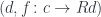rs $(d, f \colon c \to R d)$ , where $d$ is an object in $\mathcal D$ . In other words, these are all the arrows emanating from $c$ whose target is in the image of $R$ . Again, the important structure is encoded in the morphisms of $c/R$ . These are the arrows in $\mathcal D$ , $h \colon d \to d'$ that make the following diagram commute in $\mathcal C$

Notice an interesting fact: we can interpret these triangles as commutation conditions in a cone whose apex is $c$ and whose base is formed by objects and morphisms in the image of $R$ . But not all objects or morphism in the image of $R$ are included. Only those morphisms that make the appropriate triangle commute–and these are exactly the morphisms that satisfy the cone condition. So the comma category builds a cone in $\mathcal C$ .

Constructing the limit

We can now take all this information about $c$ that’s been encoded in $c/R$ and move it back to $\mathcal D$ . We define a projection functor $\pi_c \colon c/R \to D$ that maps $(d, f)$ to $d$ , thus forgetting the morphism $f$ . What’s important, though, is that this functor keeps the information encoded in the morphisms of $c/R$ , because these are morphisms in $\mathcal D$ .

The image of $\pi_c$ doesn’t necessarily cover the whole of $\mathcal D$ , because not every $R d$ has arrows coming from $c$ . Similarly, only some morphisms, the ones that make the appropriate triangle in $\mathcal C$ commute, are picked by $\pi_c$ . But those objects and morphisms that are in the image of $\pi_c$ form a diagram in $\mathcal C$ . This diagram is our partial hologram, and we can use it to pick an object in $\mathcal D$ that looks almost exactly like $c$ . That object is the limit of this diagram. We pick the limit of this diagram as the definition of $L c$ : the left adjoint of $R$ acting on $c$ .

Here’s the tricky part: we assumed that $\mathcal D$ was small-complete, so every small diagram has a limit; but the diagram defined by $\pi_c$ is not necessarily small. Let’s ignore this problem for a moment, and continue sketching the proof. We want to show that the mapping that assigns the limit of $\pi_c$ to every $c$ is left adjoint to $R$ .

Let’s see if we can define the unit of the adjunction:

$\eta_c : c \to R L c$

Since we have defined $L c$ as the limit of the diagram $\pi_c$ and $R$ preserves limits (small limits, really; but we are ignoring size problems for the moment) then $R L c$ must be the limit of the diagram $R \pi_c$ in $\mathcal C$ . But, as we noted before, the diagram $R \pi_c$ is exactly the base of the cone with the apex $c$ that we used to define the comma category $c/R$ . Since $R L c$ is the limit of this diagram, there must be a unique morphism from any other cone to it. In particular there must be a morphism from $c$ to it, because $c$ is an apex of the cone defined by the comma category. And that’s the morphism we’ll chose as our $\eta_c$ .

Incidentally, we can interpret $\eta_c$ itself as an object of the comma category $c/R$ , namely the one defined by the pair 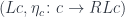$(Lc, \eta_c \colon c \to R L c)$ . In fact, this is the initial object in that category. If you pick any other object, say, 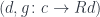$(d, g \colon c \to R d)$ , you can always find a morphism $h \colon L c \to d$ , which is just a leg, a projection, in the limiting cone that defines $L c$ . It is automatically a morphism in $c/R$ because the following triangle commutes:

This is the triangle that defines $\eta_c$ as a morphism of cones, from the top cone with the apex $c$ , to the bottom (limiting) cone with the apex $R L c$ . We’ll use this interpretation later, when discussing the full version of the Freyd’s theorem.

We can also define the counit of the adjunction. Its component at $c$ is a morphism

$\epsilon_d : L R d \to d$

First, we repeat our construction starting with $c = R d$ . We define the comma category $R d / R$ and use $\pi_{R d}$ to create the diagram whose limit is $L R d$ . We pick $\epsilon_d$ to be a projection in the limiting cone. We are guaranteed that $d$ is in the base of the cone, because it’s the image of $(d, id \colon R d \to R d)$ under $\pi_{R d}$ .

To complete this proof, one should show that the unit and counit are natural transformations and that they satisfy triangle identities.

End of a comma category

An interesting insight into this construction can be gained using the end calculus. In my previous post, I talked about (weighted) colimits as coends, but the same argument can be dualized to limits and ends. For instance, this is our comma category as a category of elements in the coend notation:

$c/R \cong \mathcal{D} \int^d \mathcal{C} (c, R d)$

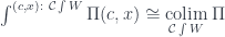
The limit of of the projection functor $\pi_c$ over the comma category can be written in the end notation as

$\lim_{c/R} \pi_c \cong \int_{(d, f)\colon c/R} \pi_c (d, f) \cong \int_{(d, f)\colon c/R} d$

This, in turn, can be rewritten as a weighted limit, with every $d$ weighted by the set $\mathcal{C}(c, R d)$ :

$\mbox{lim}^{\mathcal{C}(c, R -)} \mbox{Id} \cong \int_{d \colon \mathcal{D}} \mathcal{C}(c, R d) \pitchfork d$

The pitchfork here is the power (cotensor) defined by the equation

$\mathcal{D}\big(d', s \pitchfork d\big) \cong Set\big(s, \mathcal{D}(d', d)\big)$

You may think of $s \pitchfork d$ as the product of $s$ copies of the object $d$ , where $s$ is a set. The name power conveys the idea of iterated multiplication. Or, since power is a special case of exponentiation, you may think of $s \pitchfork d$ as a function object imitating mappings from $s$ to $d$ .

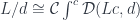
To continue, if the left adjoint $L$ exists, the weighted limit in question can be replaced by

$\int_{d \colon \mathcal{D}} \mathcal{D}(L c, d) \pitchfork d$

which, using standard calculus of ends (see Appendix), can be shown to be isomorphic to $L c$ . We end up with:

$\lim_{c/R} \pi_c \cong L c$

Solution set condition

So what about those pesky size issues? It’s one thing to demand the existence of all small limits, and a completely different thing to demand the existence of large limits (such requirement may narrow down the available categories to preorders). Since the comma category may be too large, maybe we can cut it down to size by carefully picking up a (small) set of objects out of all objects of $\mathcal D$ . We may take some indexing set $I$ and construct a family $d_i$ of objects of $\mathcal D$ indexed by elements of $I$ . It doesn’t have to be one family for all—we may pick a different family for every object $c$ for which we are performing our construction.

Instead of using the whole comma category $c/R$ , we’ll limit ourselves to a set of arrows $f_i \colon c \to R d_i$ . But in a comma category we also have morphisms between arrows. In fact they are the essential carriers of the structure of the comma category. Let’s have another look at these morphisms.

This commuting condition can be re-interpreted as a factorization of $g$ through $f$ . It so happens that every morphism $g$ can be trivially factorized through some $f$ by picking $d = d'$ and $h = id_d$ . But if we restrict the factors $f$ to be members of the family $f_i$ then not every $g \colon c \to R d$ (for arbitrary $d$ ) can be automatically factorized. We have to demand it. That gives us the following:

Solution Set Condition: For every object $c$ there exists a small set $I$ with an $I$ -indexed family of objects $d_i$ in $\mathcal D$ and a family of morphisms $f_i \colon c \to R d_i$ , such that every morphism $g \colon c \to R d$ can be factored through one of $f_i$ . That is, there exists a morphism $h \colon d_i \to d$ such that

$g = R h \circ f_i$

There is a shorthand for this statement: All comma categories $c/R$ admit weakly initial families of objects. We’ll come back to it later.

Freyd’s theorem

We can now formulate:

Freyd’s Adjoint Functor Theorem: If $\mathcal D$ is a locally small and small-complete category, and the functor $R \colon D \to C$ is continuous (small-limit preserving), and it satisfies the solution set condition, then $R$ has a left adjoint.

We’ve seen before that the key to defining the point-wise left adjoint was to find the initial object in the comma category $c/R$ . The problem is that this comma category may be large. So the trick is to split the proof into two parts: first defining a weakly initial object, and then constructing the actual initial object using equalizers. A weakly initial object has morphisms to every object in the category but, unlike its strong version, these morphisms don’t have to be unique.

An even weaker notion is that of a weakly initial set of objects. These are objects that among themselves have arrows to every object in the category, but it’s possible that no individual object has all the arrows. The solution set in Freyd’s theorem is such a weakly initial set in the comma category $c/R$ . Since we assumed that $\mathcal C$ is small-complete, we can take a product of these objects and show that it’s weakly initial. The proof then proceeds with the construction of the initial object.

The details of the proof can be found in any category theory text or in nLab.

Next we’ll see the application of these results to the problem of defunctionalization of computer programs.

Appendix

To show that

$\int_d \mathcal{D}(L c, d) \pitchfork d \cong L c$

it’s enough to show that the hom-functors from an arbitrary object $d'$ are isomorphic

$\begin{aligned} & \mathcal{D}\big(d', \int_d \mathcal{D}(L c, d) \pitchfork d\big) \\ \cong & \int_d \mathcal{D}\big(d', \mathcal{D}(L c, d) \pitchfork d\big) \\ \cong & \int_d Set\big( \mathcal{D}(L c, d), \mathcal{D}(d', d) \big) \\ \cong & \; \mathcal{D}(d', L c) \end{aligned}$

I used the continuity of the hom-functor, the definition of the power (cotensor) and the ninja Yoneda lemma.

July 20, 2020

Weighted Colimits

Posted by Bartosz Milewski under Programming
1 Comment

It’s funny how similar ideas pop up in different branches of mathematics. Calculus, for instance, is built around metric spaces (or, more generally, Banach spaces) and measures. A limit of a sequence is defined by points getting closer and closer together. An integral is an area under a curve. In category theory, though, we don’t talk about distances or areas (except for Lawvere’s take on metric spaces), and yet we have the abstract notion of a limit, and we use integral notation for ends. The similarities are uncanny.

This blog post was inspired by my trying to understand the idea behind the Freyd’s adjoint functor theorem. It can be expressed as a colimit over a comma category, which is a special case of a Grothendieck fibration. To understand it, though, I had to get a better handle on weighted colimits which, as I learned, were even more general than Kan extensions.

Category of elements as coend

Grothendieck fibration is like splitting a category in two orthogonal directions, the base and the fiber. Fiber may vary from object to object (as in dependent types, which are indeed modeled as fibrations).

The simplest example of a Grothendieck fibration is the category of elements, in which fibers are simply sets. Of course, a set is also a category—a discrete category with no morphisms between elements, except for compulsory identity morphisms. A category of elements is built on top of a category $\mathcal{C}$ using a functor

$F \colon \mathcal{C} \to Set$

Such a functor is traditionally called a copresheaf (this construction works also on presheaves, $\mathcal{C}^{op} \to Set$ ). Objects in the category of elements are pairs $(c, x)$ where $c$ is an object in $\mathcal{C}$ , and $x \in F c$ is an element of a set.

A morphism from $(c, x)$ to $(c', x')$ is a morphism $f \colon c \to c'$ in $\mathcal{C}$ , such that $(F f) x = x'$ .

There is an obvious projection functor that forgets the second component of the pair

$\Pi \colon (c, x) \mapsto c$

(In fact, a general Grothendieck fibration starts with a projection functor.)

You will often see the category of elements written using integral notation. An integral, after all, is a gigantic sum of tiny slices. Similarly, objects of the category of elements form a gigantic sum (disjoint union) of sets $F c$ . This is why you’ll see it written as an integral

$\int^{c \colon \mathcal{C}} F c$

However, this notation conflicts with the one for conical colimits so, following Fosco Loregian, I’ll write the category of elements as

$\mathcal{C}\int^{c} F c$

An interesting specialization of a category of elements is a comma category. It’s the category $L/d$ of arrows originating in the image of the functor $L \colon \mathcal{C} \to \mathcal{D}$ and terminating at a fixed object $d$ in $\mathcal{D}$ . The objects of $L/d$ are pairs $(c, f)$ where $c$ is an object in $\mathcal{C}$ and $f \colon L c \to d$ is a morphism in $\mathcal{D}$ . These morphisms are elements of the hom-set $\mathcal{D}(L c , d)$ , so the comma category is just a category of elements for the functor $\mathcal{D}(L-, d) \colon \mathcal{C}^{op} \to Set$

$L/d \cong \mathcal{C}\int^{c} \mathcal{D}(L c, d)$

You’ll mostly see integral notation in the context of ends and coends. A coend of a profunctor is like a trace of a matrix: it’s a sum (a coproduct) of diagonal elements. But (co-)end notation may also be used for (co-)limits. Using the trace analogy, if you fill rows of a matrix with copies of the same vector, the trace will be the sum of the components of the vector. Similarly, you can construct a profunctor from a functor by repeating the same functor for every value of the first argument $c'$ :

$P(c', c) = F c$

The coend over this profunctor is the colimit of the functor, a colimit being a generalization of the sum. By slight abuse of notation we write it as

$\mbox{colim}\, F = \int^{c \colon \mathcal{C}} F c$

This kind of colimit is called conical, as opposed to what we are going to discuss next.

Weighted colimit as coend

A colimit is a universal cocone under a diagram. A diagram is a bunch of objects and morphisms in $\mathcal{C}$ selected by a functor $D \colon \mathcal{J} \to \mathcal{C}$ from some indexing category $\mathcal{J}$ . The legs of a cocone are morphisms that connect the vertices of the diagram to the apex $c$ of the cocone.

For any given indexing object $j \colon \mathcal{J}$ , we select an element of the hom-set $\mathcal{C}(D j, c)$ , as a wire of the cocone. This is a selection of an element of a set (the hom-set) and, as such, can be described by a function from the singleton set $*$ . In other words, a wire is a member of $Set(*, \mathcal{C}(D j, c))$ . In fact, we can describe the whole cocone as a natural transformation between two functors, one of them being the constant functor $1 \colon j \mapsto *$ . The set of cocones is then the set of natural transformations:

$[\mathcal{J}^{op}, Set](1, \mathcal{C}(D -, c))$

Here, $[J^{op}, Set]$ is the category of presheaves, that is functors from $\mathcal{J}^{op}$ to $Set$ , with natural transformations as morphisms. As a bonus, we get the cocone triangle commuting conditions from naturality.

Using singleton sets to pick morphisms doesn’t generalize very well to enriched categories. For conical limits, we are building cocones from zero-thickness wires. What we need instead is what Max Kelly calls cylinders obtained by replacing the constant functor $1\colon \mathcal{J}^{op} \to Set$ with a more general functor $W \colon \mathcal{J}^{op} \to Set$ . The result is a weighted colimit (or an indexed colimit, as Kelly calls it), $\mbox{colim}^W D$ . The set of weighted cocones is defined by natural transformations

$[\mathcal{J}^{op}, Set](W, \mathcal{C}(D -, c))$

and the weighted colimit is the universal one of these. This definition generalizes nicely to the enriched setting (which I won’t be discussing here).

Universality can be expressed as a natural isomorphism

$[\mathcal{J}^{op}, Set](W, \mathcal{C}(D -, c)) \cong \mathcal{C}(\mbox{colim}^W D, c)$

We interpret this formula as a one-to-one correspondence: for every weighted cocone with the apex $c$ there is a unique morphism from the colimit to $c$ . Naturality conditions guarantee that the appropriate triangles commute.

A weighted colimit can be expressed as a coend (see Appendix 1)

$\mbox{colim}^W D \cong \int^{j \colon \mathcal{J}} W j \cdot D j$

The dot here stands for the tensor product of a set by an object. It’s defined by the formula

$\mathcal{C}(s \cdot c, c') \cong Set(s, \mathcal{C}(c, c'))$

If you think of $s \cdot c$ as the sum of $s$ copies of the object $c$ , then the above asserts that the set of functions from a sum (coproduct) is equivalent to a product of functions, one per element of the set $s$ ,

$(\coprod_s c) \to c' \cong \prod_s (c \to c')$

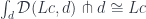
Right adjoint as a colimit

A fibration is like a two-dimensional category. Or, if you’re familiar with bundles, it’s like a fiber bundle, which is locally isomorphic to a cartesian product of two spaces, the base and the fiber. In particular, the category of elements $\mathcal{C} \int W$ is, roughly speaking, like a bundle whose base is the category $\mathcal{C}$ , and the fiber is a ( $c$ -dependent) set $W c$ .

We also have a projection functor on the category of elements $\mathcal{C} \int W$ that ignores the $W c$ component

$\Pi \colon (c, x) \mapsto c$

The coend of this functor is the (conical) colimit

$\int^{(c, x) \colon \mathcal{C}\int W} \Pi (c, x) \cong \underset{\mathcal{C} \int W}{\mbox{colim}} \; \Pi$

But this functor is constant along the fiber, so we can “integrate over it.” Since fibers depends on $c$ , different objects end up weighted differently. The result is a coend over the base category, with objects $c$ weighted by sets $W c$

$\int^{(c, x) \colon \mathcal{C}\int W} \Pi (c, x) \cong \int^{(c, x) \colon \mathcal{C}\int W} c \cong \int^{c \colon \mathcal{C}} W c \cdot c$

Using a more traditional notation, this is the formula that relates a (conical) colimit over the category of elements and a weighted colimit of the identity functor

$\underset{\mathcal{C} \int W}{\mbox{colim}} \; \Pi \cong \mbox{colim}^W Id$

There is a category of elements that will be of special interest to us when discussing adjunctions: the comma category for the functor $L \colon \mathcal{C} \to \mathcal{D}$ , in which the weight functor is the hom-functor $\mathcal{D}(L-, d)$

$L/d \cong \mathcal{C}\int^{c} \mathcal{D}(L c, d)$

If we plug it into the last formula, we get

$\underset{L/d}{\mbox{colim}} \; \Pi \cong \underset{C \int \mathcal{D}(L-, d)}{\mbox{colim}} \; \Pi \cong \int^{c \colon \mathcal{C}} \mathcal{D}(L c, d) \cdot c$

If the functor $L$ has a right adjoint

$\mathcal{D}(L c, d) \cong \mathcal{C}(c, R d)$

we can rewrite this as

$\underset{L/d}{\mbox{colim}} \; \Pi \cong \int^{c \colon \mathcal{C}} \mathcal{C}(c, R d) \cdot c$

and useing the ninja Yoneda lemma (see Appendix 2) we get a formula for the right adjoint in terms of a colimit of a comma category

$\underset{L/d}{\mbox{colim}} \; \Pi \cong R d$

Incidentally, this is the left Kan extension of the identity functor along $L$ . (In fact, it can be used to define the right adjoint as long as it preserves the functor $L$ .)

We’ll come back to this formula when discussing the Freyd’s adjoint functor theorem.

Appendix 1

I’m going to prove the following identity using some of the standard tricks of coend calculus

$\mbox{colim}^W D \cong \int^{j \colon \mathcal{J}} W j \cdot D j$

To show that two objects are isomorphic, it’s enough to show that their hom-sets to any object $c'$ are isomorphic (this follows from the Yoneda lemma)

$\begin{aligned} \mathcal{C}(\mbox{colim}^W D, c') & \cong [\mathcal{J}^{op}, Set]\big(W-, \mathcal{C}(D -, c')\big) \\ &\cong \int_j Set \big(W j, \mathcal{C}(D j, c')\big) \\ &\cong \int_j \mathcal{C}(W j \cdot D j, c') \\ &\cong \mathcal{C}(\int^j W j \cdot D j, c') \end{aligned}$

I first used the universal property of the colimit, then rewrote the set of natural transformations as an end, used the definition of the tensor product of a set and an object, and replaced an end of a hom-set by a hom-set of a coend (continuity of the hom-set functor).

Appendix 2

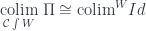
The proof of

$\int^{c \colon \mathcal{C}} \mathcal{C}(c, R d) \cdot c \cong R d$

follows the same pattern

$\begin{aligned} &\mathcal{C}\Big( \big(\int^{c} \mathcal{C}(c, R d) \cdot c\big) , c'\Big)\\ \cong &\int_c \mathcal{C}\big( \mathcal{C}(c, R d) \cdot c , c'\big) \\ \cong &\int_c Set\big( \mathcal{C}(c, R d) , \mathcal{C}(c, c')\big) \\ \cong & \; \mathcal{C}(R d, c') \end{aligned}$

I used the fact that a hom-set from a coend is isomorphic to an end of a hom-set (continuity of hom-sets). Then I applied the definition of a tensor. Finally, I used the Yoneda lemma for contravariant functors, in which the set of natural transformations is written as an end.

$[ \mathcal{C}^{op}, Set]\big(\mathcal{C}(-, x), H \big) \cong \int_c Set \big( \mathcal{C}(c, x), H c \big) \cong H x$

Bartosz Milewski's Programming Cafe