July 2019

Monthly Archive

July 4, 2019

Filtered Colimits

Posted by Bartosz Milewski under Programming
1 Comment

Previously we were exploring universal constructions for products, coproducts, and exponentials. In particular, we were able to prove the distributive law:

$(a + b) \times c \cong a \times c + b \times c$

The power of this law is that it relates the mapping-in universal construction (product on the left) with the mapping-out one (coproduct on the right). If you take into account that products and coproducts are just special cases of limits and colimits, you may ask a more general question: under what conditions limits commute with colimits. In a cartesian closed category a product of sums is not equal to the sum of products:

$(a + b) \times (c + d) \ncong a \times c + b \times d$

So, in general, products don’t commute with coproducts. But if you replace coproducts with a special kind of colimits, then it can be shown that:
Theorem.
In $Set$ , filtered colimits commute with finite limits.

In this post I’ll try to explain these terms and provide some intuition why it works and how filtered colimits are related to the more traditional notion of limits that we know from calculus.

Limits

Let’s start with limits. They are like products, except that, instead of just two objects at the bottom, you have any number of objects plus a bunch of morphisms between them. That’s called a diagram. Then you have an apex with arrows going down to all the objects in the diagram; and you get what is called a cone. If you have morphisms in your diagram, they form triangles. These triangles must commute. For instance, in Fig 1, we have:

$g \circ \pi_1 = \pi_3$

Fig. 1. A cone

This means that not all projections are independent–that you may obtain one projection from another by post-composing it with a morphism from the diagram. In Fig 1, for instance, you may extract a value of $c$ either directly using $\pi_3$ or by applying $g$ to the result of $\pi_1$ .

A limit is defined as the universal cone with the apex $Lim$ . It means that, if you have any other cone with some apex $c$ , built over the same diagram, there is a unique morphism $h$ from $c$ to $Lim$ that makes all the triangles commute. For instance, in Fig 2, one of the commuting conditions is:

$\pi_1 \circ h = f_1$

and so on. We’ve seen similar commuting conditions in the definition of the product.

Fig. 2. A universal cone

If you think of $Lim$ in this example as a data structure, you would implement it as a product of $a_1$ , $a_2$ , and $a_3$ , together with two functions:

$g_3 : a_1 \to a_3$

$g_2 : a_1 \to a_2$

But because of the commuting conditions, the three values stored in $Lim$ cannot be independent. If you pick a value for $a_1$ , then the values for $a_2$ and $a_3$ are uniquely determined.

A limit, just like a product, is defined by a mapping-in property. If you want to define a morphism from some $c$ to $Lim$ , you need to provide three morphisms $f_1$ , $f_2$ , and $f_3$ . However, unlike in the case of a product, these morphisms must satisfy some commuting conditions. Here, $f_3$ must be equal to $g_3 \circ f_1$ and $f_2 = g_2 \circ f_1$ . So, really, you only need to define $f_1$ , and that uniquely determines $h$ . This is why the cones in Fig 2 can be simplified, as shown in Fig 3.

Fig. 3. A simplified universal cone

Notice that the diagram essentially forms a subcategory inside the category $C$ , even if we don’t explicitly draw all the identity morphisms or all the compositions. This is because triangles built by composing commuting triangles are again commuting. It therefore makes sense to define a diagram as a functor $F$ from an (often much smaller) index category $J$ to $C$ . In our case it would be a category with just three objects, $j_1$ , $j_2$ , $j_3$ , and two non-identity morphisms. (The diagram category for the product is even simpler: just two objects, no non-trivial morphisms.)

The properties of the diagram category determine the nature of cones and the nature of the limits. For instance, functors from a finite category will produce finite limits.

Fig. 4. Diagram category $J$

The diagram category $J$ in our example has a very peculiar property: it has a cone for every pair of objects (it’s a cone inside $J$ , not to be confused with the cone in $C$ ). For instance, the pair $j_2$ , $j_3$ is part of the cone with the apex $j_1$ . This is also the apex for the (somewhat degenerate) cone based on $j_1$ and $j_2$ (with or without the connecting morphism). A category in which there is a cone for every finite subdiagram is called cofiltered. Limits defined by functors from cofiltered categories are called cofiltered limits.

The intuition is that cofiltered categories exhibit some kind of ordering. You may think of $j_1$ as a lower bound of $j_2$ and $j_3$ . Following these bounds, you might eventually get to some kind of roots–here it’s the object $j_1$ –and these roots will dictate the behavior of cones and the behavior of limits. Things get really interesting when the diagram category is infinite, because then there is no guarantee that you’ll ever reach a root. There is, for instance, no smallest (negative) integer, even though integers are ordered. You can begin to see parallels with traditional limits, like:

$\lim_{j \to -\infty} a_j$

That’s where these ideas originally came from.

Limits in the category of sets have a particularly simple interpretation. In $Set$ , we can use functions from the terminal object–the singleton set–to pick individual set elements.

Fig. 5. Elements of the limit

For every selection in Fig 5. of $x_1$ , $x_2$ , $x_3$ there is a unique $h(x_1, x_2, x_3)$ that picks an element in $Lim$ . But a selection of $x_1$ , $x_2$ , $x_3$ is nothing but a cone with the apex $1$ . So there is a one-to-one correspondence between elements of $Lim$ and such cones. In other words, $Lim$ is a set of apex-1 cones.

Colimits

Colimits are dual to limits–you get them by inverting all the arrows. So, instead of projections, you get injections, and the universal condition defines a mapping out of a colimit (see Fig 6).

Fig. 6. A universal cocone

If you look at the colimit as a data structure, it is similar to a coproduct, except that not all the injections are independent. In the example in Fig 6, $i_3$ and $i_2$ are determined by pre-composing $i_1$ with $g_3$ and $g_2$ , respectively. It’s not clear how to implement a colimit in Haskell, so here’s a pseudo-Haskell attempt using imaginary dependent-type syntax:

  data Colim a1 a2 a3 (g2 :: a2 -> a1) (g3 :: a3 -> a1) =
           = A1 a1 | A2 a2 | A3 a3

To deconstruct this colimit, you only need to provide one function $f_1 : a_1 \to c$ .

  h :: (a1 -> c) -> Colim a1 a2 a3 g2 g3 -> c
  h f1 (A1 a1)    = f1 a1
  h f1 (A2 a2) = f1 (g2 a2)
  h f1 (A3 a3) = f1 (g3 a3)

Granted, in a lazy language like Haskell, this would be an overkill way to store essentially just one value.

A colimit in the category of sets simplifies to a disjoint union of sets, in which some elements are identified. Suppose that the colimit $Colim_J F$ is defined by some diagram category $J$ and a functor $F : J \to Set$ . Each object $j$ in $J$ produces a set $F j$ .

Fig. 7. Colimit in Set. On the left, the diagram category $J$ .

The disjoint union of all these sets is a set whose elements are the pairs $(x, j)$ where $x \in F j$ . (Notice that the sets may overlap, but each element from the overlap will be counted as many times as the number of sets it belongs to.) Coproduct injections are then functions that take an element $x \in F j$ and map it into an element $(x, j) \in Colim_J F$ . But that doesn’t take into account the presence of morphisms in the diagram. These morphisms are mapped to functions between corresponding sets. For instance, in Fig 7, we can take an element $x \in F j_2$ . It is injected, using $i_2$ , as an element $(x, j_2) \in Colim_J F$ . But there is another path from $F j_2$ that uses $F g_2$ followed by $i_1$ . That produces $((F g_2) x, j_1)$ . If the triangle is to commute, these two must be equal. So in the actual colimit, they must be identified. In general, any two elements of the disjoint union that satisfy this relation:

$(x, j) \rightsquigarrow (x', j')\;\; \text{if}\;\; \exists_{g : j \to j'} (F g) x = x'$

must be identified. This is not an equivalence relation, but it can be extended to one (by first symmetrizing it, and then making it transitive again). A colimit is then a quotient of the disjoint union by this equivalence.

As before, I chose this example to illustrate a special type of a diagram. This is a diagram that can be obtained using a functor from a filtered category. A filtered category has this property that for any finite subdiagram, there is a cocone under it. Here, for instance, the subdiagram formed by $j_2$ and $j_3$ has a cocone with the apex $j_1$ . Again, you may think of $j_1$ as a kind of upper bound of $j_2$ and $j_3$ . If the filtered category is finite, following upper bounds will eventually lead you to some roots. And in Set, the equivalence relation will allow you shift all the elements down to those roots. But in an infinite case (think natural numbers) there may be no largest element–no root. And that brings filtered colimits closer to the intuition we have for limits in calculus. In fact, all the interesting filtered colimits are based on infinite diagrams.

Commuting Limits and Colimits

What does it mean for a limit to commute with a colimit? A single colimit is generated by a functor from some index category $I \to C$ . What we need is a bunch of such colimits so that we can take a limit over those. Therefore we need a bunch of functors $I \to C$ . Moreover, those colimits have to form a diagram. So we need another index category $J$ to parameterize those functors. Altogether, we need a functor of two arguments:

$F : I \times J \to C$

It follows that, for any given $j$ in $J$ we have a functor $F(-, j) : I \to C$ . We can take a colimit of that. Then we gather those colimits into a diagram whose shape is defined by $J$ , and then take its limit. We get:

$Lim_J (Colim_I F)$

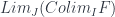
Alternatively, when we fix some $i$ in $I$ , we get a functor $F(i, -) : J \to C$ . We can take a limit of that. Then we can gather all those limits and form a diagram whose shape is defined by $I$ . Finally we can take a colimit of that:

$Colim_I (Lim_J F)$

Fig. 8. Commuting limits (red diagram of shape $J$ ) and colimits (black diagram of shape $I$ )

It’s not difficult to construct the mapping:

$Colim_I (Lim_J F) \to Lim_J (Colim_I F)$

using the universal property, since the colimit has the mapping-out property. It’s the other way around that’s tricky. But it always works in the special case when $I$ is filtered, $J$ is finite, and $C$ is $Set$ .

Here’s the sketch of this amazing proof, which you can find in Saunders Mac Lane’s Categories for the Working Mathematician.

Since the target of the functor is Set, it might help to visualize its image as a rectangular array of sets. A fixed $j$ picks up a row of such sets, whereas a fixed $i$ picks up a column. Because we are dealing with sets, we can try to define the mapping:

$Lim_J (Colim_I F) \to Colim_I (Lim_J F)$

pointwise. Let’s pick an element of the limit on the left. As we’ve established earlier, a limit in Set is a set of apex-1 cones. So let’s pick one such cone. It’s just a selection of elements from a bunch of colimits.

As we’ve seen before, a colimit in Set is a discriminated union with some identifications. So our apex-1 cone will pick a set of representatives, one per colimit, say $(x_n, i_n)$ . Any time there is a morphism $g : i_n \to i'_n$ , we can replace one representative with another $(g (x_n), i'_n)$ . The intuition is that we can slide the representatives horizontally within each row along morphisms.

If $I$ is a filtered category, then for any finite number of objects $i_n$ , we can always find a common root (it will be the apex $i$ of a cocone formed by $i_n$ in $I$ ). So we can slide all the representatives to a single column. In other words, our cone can be brought to a set of representatives $(y_n, i)$ , with a common $i$ .

Fig. 9. A single cone after shifting representatives from all colimits to a common column

But that’s just a cone over $J$ . It’s an element of $Lim_J F$ . And we can inject it into a colimit over $I$ to get an element of $Colim_I (Lim_J F)$ . We have thus defined our mapping.

Conclusion

If you didn’t get the proof the first time, don’t get discouraged. Take a break, sleep over it, and then read it slowly again. Make sure you have internalized all the definitions. Draw your own pictures. The two major tricks are: (1) visualizing an element of a limit as a cone originating from the singleton set, and (2) the idea of sliding the elements of multiple colimits to a common column.

The importance of this theorem is that it tells you when and how you can define mappings out of limits. For instance, how to define functions from a product or from an end.

Acknowledgment

I’m grateful to Derek Elkins for correcting mistakes in the original version of this post.

July 3, 2019

Programming with Universal Constructions

Posted by Bartosz Milewski under Programming
1 Comment

As functional programmers we are interested in functions. Category theorists are similarly interested in morphisms. There is a slight difference in approach, though. A programmer must implement a function, whereas a mathematician is often satisfied with the proof of existence of a morphism (unless said mathematician is a constructivist). Category theory if full of such proofs. It turns out that many of these proofs can be converted to code, often resulting in quite unexpected encodings.

A lot of objects in category theory are defined using universal constructions and universality is used all over the place to show the existence (as a rule: unique, up to unique isomorphism) of morphisms between objects.

There are two major types of universal constructions: the ones asserting the mapping-in property, and the ones asserting the mapping-out property. For instance, the product has the mapping-in property.

Product

Recall that a product of two objects $a$ and $b$ is an object $a \times b$ together with two projections:

$\pi_1 : a \times b \to a$

$\pi_2 : a \times b \to b$

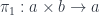
This object must satisfy the universal property: for any other object $c$ with a pair of morphisms:

$f : c \to a$

$g : c \to b$

there exists a unique morphism $h : c \to a \times b$ such that:

$f = \pi_1 \circ h$

$g = \pi_2 \circ h$

In other words, the two triangles in Fig 1 commute.

Fig. 1. Universality of the product

This universal property can be used any time you need to find a morphism that’s mapping into the product, and it can actually produce code.

For instance, let’s say you want to find a morphism from the terminal object $1$ to $a \times b$ . All you need is to define two morphisms $x : 1 \to a$ and $y : 1 \to b$ . This is not always possible, but if it is, you are guaranteed the existence of a morphism $h : 1 \to a \times b$ (Fig 2).

Fig. 2. Global element of a product

Morphisms from the terminal object are called global elements, so we have just shown that, as long as $a$ and $b$ have global elements, say $x$ and $y$ , their product has a global element too. Moreover the projection $\pi_1$ of this global element is the same as $x$ , and $\pi_2$ is the same as $y$ . In other words, an element of a product is a pair of elements. But you probably knew that.

The universal construction of the product is implemented as an operator in Haskell:

  (&&&) :: (c->a) -> (c->b) -> (c -> (a, b))

We can also go the other way: given a mapping-in $h : c \to a \times b$ , we can always extract a pair of morphisms:

$f = \pi_1 \circ h$

$g = \pi_2 \circ h$

This bijection between $h$ and a pair of morphisms $(f, g)$ is in fact an adjunction.

You might think this kind of reasoning is very different from what programmers do, but it’s not. Here’s one possible definition of a product in Haskell (besides the built-in one, (,)):

  data Product a b = MkProduct { fst :: a
                               , snd :: b }

It is in one-to-one correspondence with what I’ve just explained. The two functions fst and snd are $\pi_1$ and $\pi_2$ , and MkProduct corresponds to our $h : 1 \to a \times b$ . The categorical definition is just a different, much more general, way of saying the same thing.

Here’s another application of universality: Show that product is functorial. Suppose that you have a pair of morphisms:

$f : a \to a'$

$g : b \to b'$

and you want to lift them to a morphism:

$h : a \times b \to a' \times b'$

Since we are dealing with products, we should use the mapping-in property. So we draw the universality diagram for the target $a' \times b'$ , and put the source $a \times b$ at the top. The pair of functions that fits the bill is $(f \circ \pi_1, g \circ \pi_2)$ (Fig 3).

Fig. 3. Functoriality of the product

The universal property gives us, uniquely, the $h$ , which is usually written simply as $f \times g$ .

Exercise for the reader: Show, using universality, that categorical product is symmetric.

Coproduct

The coproduct, being the dual of the product, is defined by the universal mapping-out property, see Fig 4.

Fig. 4. Universality of the coproduct

So if you need a morphism from a coproduct $a + b$ to some $c$ , it’s enough to define two morphisms:

$f : a \to c$

$g : b \to c$

This universal property may also be restated as the isomorphism between pairs of morphisms $(f, g)$ and morphisms of the type $a+b \to c$ (so there is, in fact, a corresponding adjunction).

This is easily illustrated in Haskell:

  h :: Either a b -> c
  h (Left a)  = f a
  h (Right b) = g b

Here Left and Right correspond to the two injections $i_1$ and $i_2$ . There is a convenient function in Haskell that encapsulates this universal construction:

  either :: (a->c) -> (b->c) -> (Either a b -> c)

Exercise for the reader: Show that coproduct is functorial.

So next time you ask yourself, what can I do with a universal construction? the answer is: use it to define a morphism, either mapping in or mapping out of your construct. Why is it useful? Because it decomposes a problem into smaller problems. In the examples above, the problem of constructing one morphism $h$ was nicely decomposed into defining $f$ and $g$ separately.

The flip side of this is that there is no simple way of defining a mapping out of a product or a mapping into a coproduct.

Distributive Law

For instance, you might wonder if the familiar distributive law:

$(a + b) \times c \cong a \times c + b \times c$

holds in an arbitrary category that defines products and coproducts (so called bicartesian category). You can immediately see that defining a morphism from right to left is easy, because it involves the mapping out of a coproduct. All we need is to define a pair of morphisms leading to the common target (Fig 5):

$f : a \times c \to (a + b) \times c$

$g : b \times c \to (a + b) \times c$

Fig. 5. Right to left proof

The trick is to take advantage of the functoriality of the product, which we have already established, and use it to implement $f$ and $g$ as:

$f = i_1 \times id_c$

$g = i_2 \times id_c$

But if you try to construct a proof in the other direction, from left to right, you’re stuck, because it would require the mapping out of a product. So the distributive property does not hold in general.

“Wait a moment!” I hear you say, “I can easily implement it in Haskell.”

  f :: (Either a b, c) -> Either (a, c) (b, c)
  f (Left a, c)  = Left  (a, c)
  f (Right b, c) = Right (b, c)

Exponential

That’s correct, but Haskell does a little cheating behind the scenes. You can see it clearly when you convert this code to point free notation (I’ll explain later how I figured it out):

  f = uncurry (either (curry Left) (curry Right))

I want to direct your attention to the use of curry and uncurry. Currying is the application of another universal construction, namely that of the exponential object $c^b$ , representing the function type b -> c. This is exactly the construction that provides the missing mapping out of a product, (a, b) -> c. Here we go:

  uncurry :: (c -> (a -> b)) -> ((c, a) -> b)

Categorically, we have the bijection between morphisms (again, a sign of an adjunction):

$h : c \to b^a$

$f : c \times a \to b$

Universality tells us that for every $c$ and $f$ there is a unique $h$ in Fig 6 (and vice versa). The arrow $h \times id_a$ is the lifting of the pair $(h, id_a)$ by the product functor (we’ve established the functoriality of the product earlier).

Fig. 6. Universality of the exponential

Not every category has exponentials–the ones that do are called cartesian closed (cartesian, because they must also have products).

So how does the fact that we have exponentials in Haskell help us here? We are trying to define a mapping out of a product:

$f : (a + b) \times c \to a \times c + b \times c$

Here’s where the exponential saves the day. This mapping exists if we can define another mapping:

$h : (a + b) \to (a \times c + b \times c)^c$

see Fig 7.

Fig. 7. Uncurrying

This morphism, in turn, is easy to define, because it involves a mapping out of a sum. We just need a pair of morphisms:

$h_1 : a \to (a \times c + b \times c)^c$

$h_2 : b \to (a \times c + b \times c)^c$

We can define the first morphism using the universal property of the exponential, picking the injection $i_1$ :

Fig. 8. Defining $h_1$

This translates to Haskell as h1 = curry Left. Similarly for $h_2$ we get curry Right.

We can now combine all these diagrams into a single point-free definition, and that’s exactly how I came up with the original code:

  f = uncurry (either (curry Left) (curry Right))

Notice that curry is used to get from $f$ to $h$ , and uncurry from $h$ to $f$ in the original diagram.

Products and coproducts are examples of more general constructions called limits and colimits. Importantly, the universal property of limits can be used to define the mapping-in morphisms, whereas the universal property of colimits allows us to define the mapping-out morphisms. I’ll talk more about it in the upcoming post.

Bartosz Milewski's Programming Cafe