Bartosz Milewski's Programming Cafe

July 11, 2026

Tambara Equipment

Posted by Bartosz Milewski under Category Theory, Double category | Tags: Category Theory, Double Categories, Optics, Proarrow Equipment, Profunctors, Tambara Modules |
[2] Comments

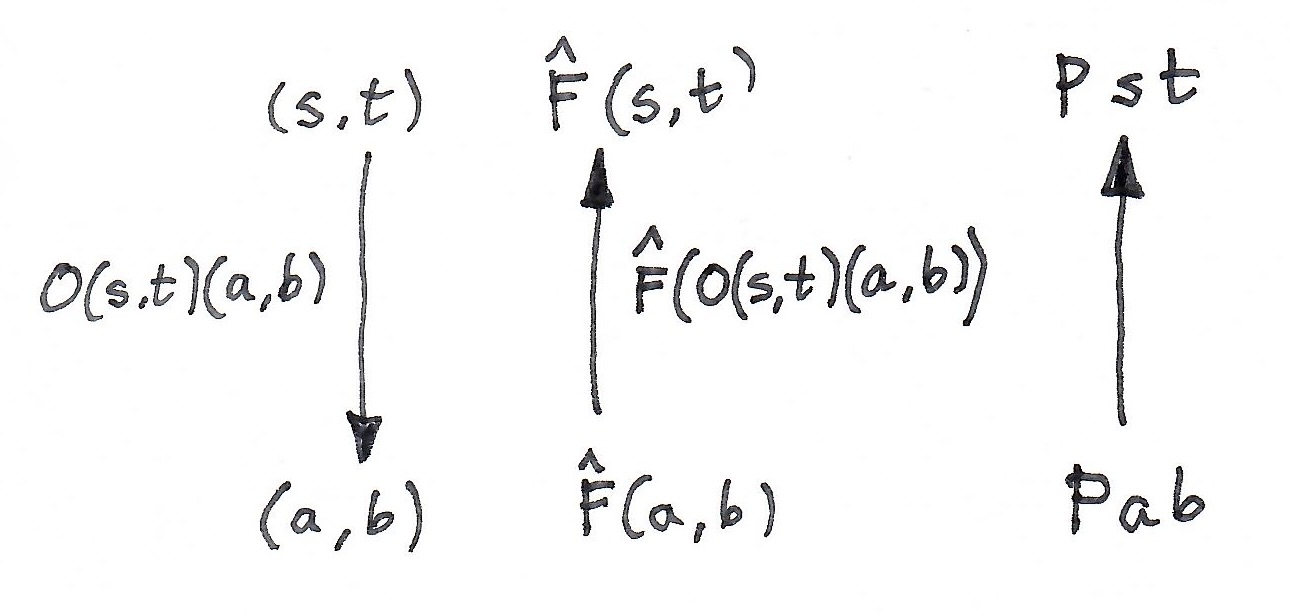
I was originally attracted to category theory when trying to understand Haskell optics. I was puzzled by the van Laarhoven’s functor representations and Kmett’s use of Tambara modules. By playing Tetris with the Yoneda lemma I was able to make some progress, attacking more and more esoteric topics. With a group of researcher and students at the Oxford Adjoint School in Applied Category Theory we cracked the problem of traversal optics and published a paper summarizing the advances in profunctor optics.

Optics sit at an intersection of monoidal actions and Tambara modules. There is a duality between optics and Tambara representations. It is related to what mathematicians call Tannakian reconstruction, when an algebraic object is recovered from the totality of its representations.

No wonder then that a recent article by Mateusz Stroiński, Module categories, internal bimodules and Tambara modules, piqued my interest. It turns out that Tambara modules can be thought of as horizontal arrows in a double category, which is also a proarrow equipment. I will try to sketch the contents of this paper and illustrate it using Haskell code.

The slogan is that Tambara modules are to monoidal functors as profunctors are to functors.

The main advantage of the double-categorical setting for Tambara modules is that it works out of the box for enriched categories.

Monoidal functors redux

For simplicity, I’ll be using a simplified version of a strict monoidal functor, which omits the object constraint from the definition of a monoidal category:

			
class (Actegory ten act1, Actegory ten act2, Functor f) =>
  MonFunctor ten act1 act2 f where
    alpha  :: m `act2` f a -> f (m `act1` a)
    alpha' :: f (m `act1` a) -> m `act2` f a

Here, alpha' is the inverse of alpha.

Monoidal functors compose:

			
newtype MonFunCompose f g a = 
  MonFunCompose { getMonFunCompose :: f (g a) }

and the composition is again a monoidal functor:

			
instance ( Actegory ten act1
         , Actegory ten act2
         , Actegory ten act3
         , MonFunctor ten act2 act3 f
         , MonFunctor ten act1 act2 g) 
        => MonFunctor ten act1 act3 (MonFunCompose f g)
  where
    alpha mfga = 
        let m3fga' = second getMonFunCompose mfga
            fmga = alpha @ten @act2 @act3 m3fga'
            fgma = fmap (alpha @ten @act1 @act2) fmga
        in MonFunCompose fgma
    alpha' (MonFunCompose fgma) = 
        let fmga = fmap (alpha' @ten @act1 @act2) fgma
            mfga = alpha'  @ten @act2 @act3 fmga 
        in  second MonFunCompose mfga
  

		

Notice the use of type application to help the Haskell type checker.

Tambara modules

A Tambara module is a profunctor that is compatible with the action of a monoidal category. If you interpret a profunctor as a proof-relevant relation, a Tambara module has the property that, whenever two objects are related, they remain related when you “multiply” them by the same object $m$ . Multiplication in this case means the action of a monoidal category $\mathbf M$ . In other words, a Tambara module is a profunctor $J \colon A^{op} \times B \to \mathbf{Set}$ equipped with the transformation:

$\lambda_{m a b} \colon J a b \to J (m \triangleright_1 a) (m \triangleright_2 b)$

that is natural in $a$ and $b$ , and dinatural in $m$ . The action interacts nicely with the monoidal structure:

$\lambda_{(m \otimes n) a b} = \lambda_{m (n \triangleright a) (n \triangleright b)} \circ \lambda_{n a b}$

$\lambda_{1 a b} = id$

(modulo some associators and unitors).

We can illustrate this in Haskell as a typeclass:

			
class (Actegory ten act, Profunctor j) 
  => Tambara ten act j where
    leftAct :: j a b -> j (m `act` a) (m `act` b)

I chose to concentrate on the left action of the actegory, but it’s easy to define the right action, or both. For simplicity, I’m using the same action for both arguments. In full generality, we would have two separate actegories.

The simplest example of a Tambara module is the hom-functor:

			
instance (Actegory ten act) => Tambara ten act (->) where
    leftAct :: Actegory ten act => (a -> b) -> m `act` a -> m `act` b
    leftAct = second

Here I used the bifunctoriality of the action.

Tambara modules form a category, in which action-preserving natural transformations act as morphisms.

The usual profunctor composition using coends also works on Tambara modules.

			
data TamCompose p q d c where
  TamCompose :: p x c -> q d x -> TamCompose p q d c

The result of composition is again a Tambara module:

			
instance (Tambara ten act p, Tambara ten act q) 
  => Tambara ten act (TamCompose p q) where
    leftAct :: (Tambara ten act p, Tambara ten act q) =>
        TamCompose p q a b -> TamCompose p q (m `act` a) (m `act` b)
    leftAct (TamCompose pxc qdx) 
      = TamCompose (leftAct pxc) (leftAct qdx)
    

		

Taken together, we have a bicategory $\mathbf{Tam}$ , where actegories are 0-cells, Tambara modules with coend composition are 1-cells, and natural transformations between them are 2-cells.

Moreover, endo-Tambara modules, that is Tambara modules that operate within a single category, form a monoidal bicategory, with profunctor composition acting as a tensor product and a hom-functor acting as a unit.

Tambara Equipment

We have previously studied a double category $\mathbb{P}rof$ in which categories are 0-cells, profunctors are horizontal arrows, functors are vertical arrows, and natural transformations form 2-cells. This double category happens to be a proarrow equipment, which relates functors to representable profunctors in a specific way.

It turns out that there is an analogous construction with actegories as 0-cells, Tambara modules as horizontal 1-cells, and monoidal functors as vertical 1-cells. To form 2-cells, we first have to be able to lift (or restrict) a Tambara module along a pair of monoidal functors. We define a lifting of $J$ as the profunctor:

$\langle a, c \rangle \mapsto J(f a)(g c)$

or, using placeholders, $J(f -) (g =)$ . In Haskell this is:

newtype Lift f g j a c = Lift (j (f a) (g c))

The lifting of a Tambara module is again a Tambara module with the structure map defined as a composition:

$J (f a) (g c) \xrightarrow{\lambda_{m (f a) (g c)}} J (m \triangleright_2 f a) (m \triangleright_2 g c) \xrightarrow {J \alpha^{-1} \alpha} J (f (m \triangleright_1 a)) (g (m \triangleright_1 c))$

The second arrow lifts the (invertible) monoidal functor structure map to $J$ :

$\alpha \colon m \triangleright_2 g c \to g (m \triangleright_1 c)$

Here’s the same thing in Haskell:

			
instance ( Actegory ten act1
         , Actegory ten act2
         , MonFunctor ten act1 act2 f
         , MonFunctor ten act1 act2 g
         , Tambara ten act2 j) 
    => Tambara ten act1 (Lift f g j) where
    leftAct (Lift j) = Lift $ dimap alpha' alpha $ leftAct @ten @act2 j
    

		

I used type applications to select the correct left action corresponding to act2.

A 2-cell is then a natural transformation from $H$ to the lifting of $J$ .

Or, in Haskell:

type Cell f g h j = forall a c . h a c -> j (f a) (g c)

The companion and the conjoint are representable profunctors, that are automatically Tambara modules as long as f is a monoidal functor (the Identity functor is trivially monoidal):

			
type Companion f d c = Lift f Identity (->)
type Conjoint f d c  = Lift Identity f (->)

The unit and counit cells for the companion and the conjoint are reasonably easy to define (see the linked code).

Free Tambara and Optics

There is an obvious forgetful functor from $\mathbf{Tamb}$ to $\mathbf{Prof}$ (it forgets the action). This functor has a left adjoint. For any profunctor $J$ , it produces a free Tambara module given by the following coend:

$(\Phi J) \, s t = \int^m \int^{x y} C(s, m \triangleright x) \times J x y \times C(m \triangleright y, t)$

In Haskell, we model it as an existential data type:

			
data FreeTamb ten act j s t = 
  forall m x y. (MonoidalCategory ten, Actegory ten act) 
  => FreeTamb (s -> m `act` x) (j x y) (m `act` y -> t)

The result is indeed a Tambara module:

			
instance (Actegory ten act, MonoidalCategory ten, Profunctor j) 
  => Tambara ten act (FreeTamb ten act j) where
    -- na -> (nm)c, jcd, (nm)d -> nb
    leftAct (FreeTamb a_mc jcd md_b) = FreeTamb f jcd g
      where
        --f :: n `act` a -> (n `ten` m) `act` c
        f  na = assoc' $ second a_mc na
        --g :: (n `ten` m) `act` d -> n `act` b
        g nm_d= second md_b $ assoc nm_d
  

		

It so happens that optics can be defined as a free Tambara module acting on a representable profunctor $\Theta_{a b} x y = C(x, a) \times C(b, y)$ . Indeed, applying the Yoneda reduction, we get:

$O\, s t a b = \int^{m} C(s, m \triangleright a) \times C(m \triangleright b, t)$

In Haskell

data Rep a b x y = Rep (x -> a) (b -> y)

giving us:

type Optic ten s t a b = FreeTamb ten (Rep a b) s t

which, by Yoneda reduction, is isomorphic to:

			
data Optic ten act s t a b = forall m.
    Optic (s -> m `act` a) (m `act` b -> t)

Internalizing monoidal actions

A monoidal action, seen as a functor $\mathbf M \to [C, C]$ , can be internalized in $M$ if it has a right adjoint:

$C(m \triangleright a, t) \cong \mathbf M (m, \{a, t \} )$

If you think of the action as “multiplication,” the adjunction is reminiscent of currying, and the right adjoint plays to role on the “internal hom.”

In Haskell, we define a typeclass:

			
class (Actegory ten act, MonoidalCategory ten, Profunctor hom) 
  => IntHom ten act hom | hom -> act where
    icurry   :: (m `act` a -> b) -> (m -> hom a b)
    iuncurry :: (m -> hom a b)   -> (m `act` a -> b)

We can use this adjunction to simplify multiplicative optics:

$\int^{m} C(s, m \triangleright a) \times C(m \triangleright b, t) \cong \int^{m} C(s, m \triangleright a) \times \mathbf M (m, \{b, t \})$

Using the Yoneda reduction (a.k.a, “integrating” over $m$ ), this is equivalent to:

$O \, s t a b \cong C(s, \{b, t \} \triangleright a )$

With additive optics, we use the right adjoint to coproduct to produce hom-sets in a product category.

Both tricks are used in simplifying traversals, which are optics generated by polynomial functors:

$\int^{c \colon [\mathbb N , Set]} C(s, \sum_n c_n \times a^n) \times C (\sum_m c_m \times b^m, t)$

Here, $c$ is a natural-number-indexed family of objects with a monoidal structure given by convolution; and $a^n$ and $b^n$ are powers.

We first use the coproduct adjunction:

$C (\sum_m c_m \times b^m, t) \cong \prod_m C(c_m \times b^m, t)$

and follow it by the currying adjunction. We get the formula for a traversal:

$T \, s t a b \cong Set(s, \sum_n Set(b^n, t) \times a^n)$

The result can be illustrated in Haskell by replacing powers with lists:

type Traversal s t a b = s -> ([b] -> t, [a])

Internal monoid

The endo-hom $\{a, a\}$ is automatically a monoid in $\mathbf M$ . Indeed, we can define monoid multiplication as:

$\mathbf M(\{a, a\} \otimes \{a, a\}, \{a, a\}) \cong C\big((\{a, a\} \otimes \{a, a\}) \triangleright a, a\big)$

The right hand side can be implemented as a double application of the counit of the adjunction:

$\epsilon_{a a} = \{a, a\} \triangleright a \to a$

In Haskell, we first define a monoid internal to a monoidal category:

			
class (MonoidalCategory ten) => IMonoid ten m where
    imempty  :: Unit ten -> m
    imappend :: m `ten` m -> m

and show that hom a a is an instance of it:

			
instance (Actegory ten act, MonoidalCategory ten, IntHom ten act hom)  
  => IMonoid ten (hom a a) where
    imempty = icurry unit
    -- imappend :: (hom a a) `ten` (hom a a) -> hom a a
    imappend = icurry (eval . second eval . assoc)

where counit of the adjunction is the eval function:

			
eval :: (Actegory ten act, MonoidalCategory ten, IntHom ten act hom) 
  => hom a b `act` a -> b
eval = iuncurry id

Haskell code for this blog post is available here.

June 30, 2026

Actegories

Posted by Bartosz Milewski under Category Theory, Haskell | Tags: Actegories, Category Theory, Haskell, Lens, Optics |
Leave a Comment

Previously: Kan Extensions in Double Categories.

In programming, actegories play a central role in optics: lenses, prisms, traversals, etc. To understand actegories, let’s start with the definition of a monoidal category.

Monoidal Category

A monoidal category $\mathbf M$ is a category equipped with a tensor product. A tensor product is a functor $\otimes \colon \mathbf M \times \mathbf M \to \mathbf M$ . We assume that this product is associative and unital– up to isomorphism. It means that there is an invertible associator:

$\alpha_{a, b, c} \colon (a \otimes b) \otimes c \to a \otimes (b \otimes c)$

natural in all three arguments. We also have a unit object $1$ and two (invertible, natural) unitors:

$\lambda_a \colon 1 \otimes a \to a$

$\rho_a \colon a \otimes 1 \to a$

To get a better feel for it, we can try to model a monoidal category in Haskell. We parameterize it by the type of the tensor product, ten, which we want to be a Bifunctor:

class (Bifunctor ten) => MonoidalCategory ten where ...

The standard way to define a subcategory of Hask is to restrict the types of objects by imposing a constraint. Such a restriction has a special kind, Constraint:

			
class Bifunctor ten
  => MonoidalCategory (obj :: Type -> Constraint) ten where ...

A common example of such a constraint is a typeclass. For instance Monoid will restrict the objects of the category to be monoids. (In principle, we should also restrict the type of arrows, here to monoid morphisms.)

We can specify the unit of a monoidal category as an associated type (parameterized by ten):

    type Unit ten :: Type

The unit should be an object of the category, so it should satisfy the constraint. We can encode this in our definition as a precondition: obj (Unit ten). This leads to a circularity, which we can overcome using the language pragma UndecidableSuperClasses:

			
class (Bifunctor ten , obj (Unit ten))
  => MonoidalCategory (obj :: Type -> Constraint) ten where
    type Unit ten :: Type
    ...

Finally, we can add the associator and the unitors (and their inverses):

			
class (Bifunctor ten , obj (Unit ten))
  => MonoidalCategory (obj :: Type -> Constraint) ten where
    type Unit ten :: Type
    alpha  :: (obj a, obj b, obj c) =>  (a `ten` b) `ten` c -> a `ten` (b `ten` c)
    lambda :: (obj a) => (Unit ten) `ten` a -> a
    ...

		

Notice the obj constraints in the type of these functions and the infix notation for the tensor.

Let’s work out a few examples. The simplest is the category of all types with a cartesian product as tensor.

			
instance MonoidalCategory Hask (,) where
    type Unit (,) = ()
    alpha ((a, b), c) = (a, (b, c))
    lambda ((), a) = a
    ...

		

We define Hask using an empty class, and we make all objects its instances:

			
class Hask a
instance Hask a

Similarly, we can define a monoidal category with Either as the tensor product, or with Monoid as the object constraint.

Actegory

An actegory is a category that supports the action of a monoidal category. You may think of it as “multiplying” or “scaling” the objects of this category by objects of the monoidal category. The (left) action can be defined as a functor from the product category to $C$ :

$\triangleright \colon \mathbf M \times C \to C$

or, after currying, as a functor from $\mathbf M$ to the endofunctor category:

$\triangleright \colon \mathbf M \to [C, C]$

The coherency conditions are the invertible natural transformations that relate the action $\triangleright$ to the tensor product $\otimes$ and its unit $1$ :

$\alpha_{m n a} \colon (m \otimes n) \triangleright a \to m \triangleright (n \triangleright a)$

$\lambda_{a} \colon 1 \triangleright a \to a$

The action is functorial in both arguments, so our Haskell translation pegs it, for simplicity, as a Bifunctor. (A Profunctor action is also possible. Categorically, it would correspond to using $\mathbf M^{op}$ as the monoidal category.)

			
class (MonoidalCategory obj ten, Bifunctor act) 
  => Actegory obj ten act | act -> ten where
    assoc  :: (obj m, obj n) 
           => (m `ten` n) `act` a -> m `act` (n `act` a)
    assoc' :: (obj m, obj n)
           => m `act` (n `act` a) -> (m `ten` n) `act` a
    unit   :: Unit ten `act` a -> a
    unit'  :: a -> Unit ten `act` a

		

Another simplifying assumption is that the action uniquely identifies the tensor product, encoded here as the functional dependency act -> ten.

The simplest example of an actegory is the self action of the cartesian product. Here, the monoidal category acts on itself:

			
instance Actegory Hask (,) (,) where
    assoc ((m, n), a) = (m, (n, a))
    assoc' (m, (n, a)) = ((m, n), a)
    unit ((), a) = a
    unit' a = ((), a)

		

Monoidal Functors

Actegories that use the same monoidal category for their actions form a category. The morphisms in this category are (strict) monoidal functors. These are functors that map one action to another:

$f (m \triangleright_1 a) \cong m \triangleright _2 f a$

In Haskell, we can model them as:

			
class (Actegory obj ten act1, Actegory obj ten act2, Functor f) =>
  MonFunctor obj ten act1 act2 f where
    as  :: obj m => m `act2` f a   -> f (m `act1` a)
    as' :: obj m => f (m `act1` a) -> m `act2` f a

In fact, actegories form a bicategory, with action-preserving natural transformations acting between monoidal functors.

Here’s an interesting example of a monoidal functor between non-trivial actegories:

			
instance (Traversable f) => MonFunctor Monoid (,) (,) (,) f where
    as (m, fa) = fmap (m, ) fa
    as' = sequenceA

Haskell code is available here.

June 13, 2026

Kan Extensions in Double Categories

Posted by Bartosz Milewski under Category Theory, Double category, Haskell, Kan extensions, Profunctor Equipment | Tags: Category Theory, Double Category, Profunctors |
Leave a Comment

Previously: Kan extensions in Haskell.

In a double category that is also a proarrow equipment, we have the ability to bend arrows. In particular, in the definition of the counit of the right Kan extension:

we can bend the vertical $j$ arrow, replacing it with its horizontal conjoint $B(1, j)$ . In a profunctor equipment, this is just a representable profunctor $\langle b, a\rangle \mapsto B(b, j a)$ .

A natural generalization is to replace this representable with a general profunctor. This way we get a definition of a right Kan extension along a profunctor $J$ .

In a more general setting of a double category, the counit of the right Kan extension is a 2-cell:

The universal condition can be similarly generalized by bending the $j$ arrows.

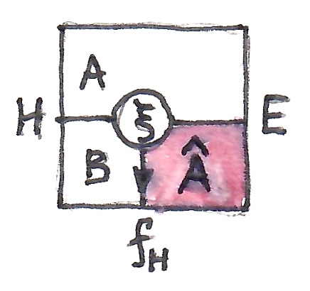
However, the universal condition for pointwise right Kan extensions is stronger. It involves an additional horizontal 1-cell $H$ . It states that any 2-cell $\phi$ of the shape below can be uniquely factorized through the counit $\epsilon$ :

Right Kan extensions in Haskell

In Haskell, the right Kan extension of a functor d along a profunctor j can be written as a data type:

newtype Ran j d a = Ran (forall x . j a x -> d x)

This is a direct translation of the categorical formula that uses an end:

$(\text{Ran}_J d) \, a = \int_x \text{Set}(J a x, d \, x)$

Compare this with the earlier implementation of the Kan extension, in which j was a functor:

newtype Ran j d a = Ran (forall x . (a -> j x) -> d x)

The counit is a 2-cell from j to the identity profunctor (->):

			
epsilon :: (Profunctor j, Functor d) => 
  Cell (Ran j d) d j (->)
epsilon jab (Ran ran) = ran jab

The 2-cell Phi goes from the profunctor composition of j and h to the identity profunctor:

type Phi s d j h  = Cell s d (Procompose j h) (->)

The factorization cell Phi' goes from h to identity:

type Phi' s d j h = Cell s (Ran j d) h (->)

For any Phi, we can find the corresponding Phi':

			
rightAdj :: (Profunctor j, Profunctor h, Functor d, Functor s) =>
        Phi s d j h -> Phi' s d j h
rightAdj phi hac sa = Ran (\ jcb -> phi (Procompose jcb hac) sa)

This function replaces the right adjoint used in the traditional definition of a Kan extension.

The result satisfies the factorization property:

			
factor :: (Profunctor j, Profunctor h, Functor d, Functor s) => 
  Phi s d j h -> Phi s d j h
factor phi = funComp . vcomp (rightAdj phi) epsilon

Here vcomp is the vertical composition of 2-cells:

			
vcomp :: (Functor f, Functor g, Functor h
         , Profunctor p, Profunctor q, Profunctor r, Profunctor s) =>
  Cell f g p r -> Cell g h q s 
  -> Cell f h (Procompose q p) (Procompose s r)
vcomp fg_pr gh_qs (Procompose qxc pax) 
    = Procompose (gh_qs qxc) (fg_pr pax)

		

and funComp is hom-functor composition:

			
funComp :: Procompose (->) (->) a b -> (a -> b)
funComp (Procompose f g) = f . g

The computational meaning of the universal construction is that, in order to define a 2-cell (natural transformation) from some functor s to Ran j d along a profunctor h, it’s enough to provide a 2-cell from s to d along a composite Procompose j h.

Left Kan extensions

We can apply similar generalization to left Kan extensions. This time we start with the unit given by the 2-cell:

The universal condition that defines the pointwise left Kan extension of a vertical 1-cell $d$ along a horizontal 1-cell $J$ is given by the following unique factorization:

Left Kan extensions in Haskell

In Haskell, we define the left Kan extension along a profunctor as an existential data type:

			
data Lan j d a where
    Lan :: j x a -> d x -> Lan j d a

This is a direct translation of the coend formula:

$(\text{Lan}_J d)\, a = \int^x ( J x a \times d \,x)$

The unit is a 2-cell:

			
eta :: (Profunctor j, Functor d) => Cell d (Lan j d) j (->)
eta jab da = Lan jab da

The universal condition states that, for any 2-cell:

type Phi s d j h  = Cell d s (Procompose h j) (->)

there is a unique 2-cell:

type Phi' s d j h = Cell (Lan j d) s h (->)

given by the mapping:

			
leftAdj :: (Profunctor j, Profunctor h, Functor d, Functor s) =>
        Phi s d j h -> Phi' s d j h
leftAdj phi hac (Lan jxa dx) = phi (Procompose hac jxa) dx

that uniquely factorizes through the unit eta:

			
factor :: (Profunctor j, Profunctor h, Functor d, Functor s) =>
    Phi s d j h -> Phi s d j h
factor phi = funComp . vcomp eta (leftAdj phi)

Again, computationally, this defines a mapping-out property of the left Kan extension.

Complete Haskell code is available here: left Kan extensions, right Kan extensions.

June 8, 2026

Kan Extensions in Haskell

Posted by Bartosz Milewski under Category Theory, Haskell, Programming | Tags: Category Theory, Haskell, Kan extensions, Universal Arrows |
1 Comment

Previously: Tabulation Tribulations.

If you think of functor composition as a form of multiplication, Kan extensions are an attempt to construct inverses of this multiplication. But unlike multiplication, composition is not symmetric, so we have extensions that attempt to undo precomposition, and lifts that do the same for postcomposition. Furthermore, there rarely is a single inverse to any form of composition, so we have the parsimonious right extensions and lifts, and the generous left extensions and lifts. We end up with four combinations that correspond to four different adjunctions:

$(- \circ j) \dashv \text{Ran}_j -$

$\text{Lan}_j - \dashv (- \circ j )$

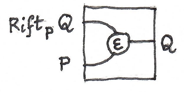
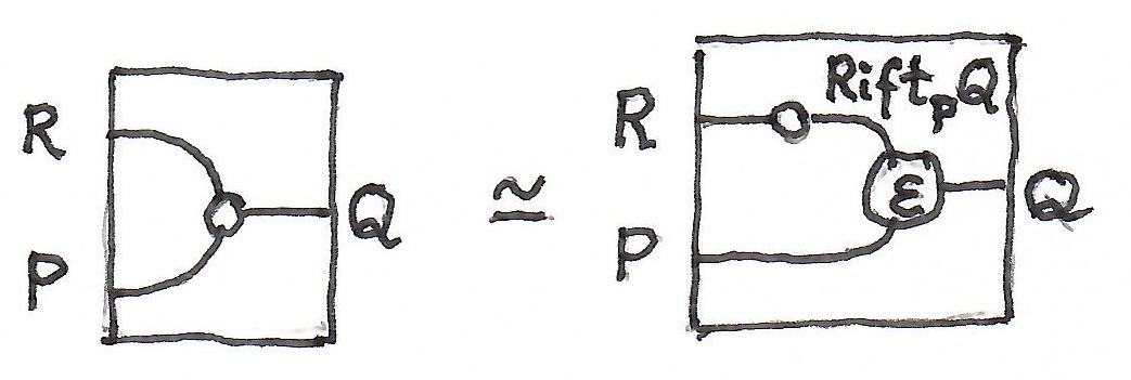
$(j \circ -) \dashv \text{Rift}_j -$

$\text{Lift}_j - \dashv (j \circ -)$

We’ll concentrate on the extensions, since we can provide explicit point-wise formulas for them in cases that are of interest to us, that is in $\mathbf{Cat}$ and in $\mathbb{P}rof$ .

Right Kan extensions

The definition of the right Kan extension relates the mapping out of the composition to the mapping into $\text{Ran}$ . In Haskell, we can define them as two types:

			
type Phi  j s d = Compose s j ~> d
type Phi' j s d = s ~> Ran j d

The wavy arrows denote natural transformations:

type f ~> g = forall x. f x -> g x

To show that there is an adjunction we can either prove the (natural) isomorphism between Phi and Phi', or implement the unit and counit of the adjunction (together with zigzag identities):

			
eta     :: (Functor j, Functor d) => d ~> Ran j (Compose d j)
epsilon :: (Functor j, Functor d) => Compose (Ran j d) j ~> d

In Haskell we can implement the right Kan extension as:

newtype Ran j d a = Ran (forall x . (a -> j x) -> d x)

This is a straightforward translation of the categorical formula that uses an end:

$(\text{Ran}_j d) \,a = \int_x \text{Set}(C(a, j \,x), d \, x)$

The adjunction can then be implemented as a pair of mappings:

			
leftAdj :: (Functor j, Functor d, Functor s) =>
   Phi j s d -> Phi' j s d
leftAdj phi sx = Ran (\x_jx -> phi (Compose (fmap x_jx sx)))
rightAdj ::  (Functor j, Functor d, Functor s) =>
   Phi' j s d -> Phi j s d
rightAdj phi' (Compose sj) = 
    let (Ran ran) = phi' sj
    in ran id

		

Or as the unit/counit pair:

			
eta :: (Functor j, Functor d) => d ~> Ran j (Compose d j)
eta dx = Ran (\x_jx -> Compose (fmap x_jx dx))
epsilon :: (Functor j, Functor d) => Compose (Ran j d) j ~> d
epsilon (Compose (Ran ran)) = ran id

Universal arrows

There is a third way, which gives a better starting point for generalizations. It can be used on an object-by-object basis, even if there is no global adjunction. It’s based on the idea of the universal arrow.

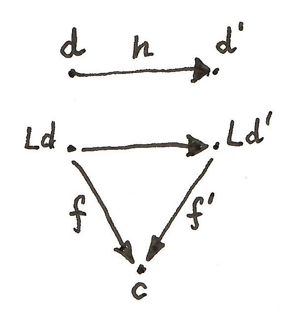
A universal arrow is a terminal object in the comma category. For a given functor $L \colon D \to C$ , the comma category $L/c$ consists of pairs $(d, f \colon L d \to c)$ . In other words, it’s a category of arrows from the image of $L$ to some fixed object $c \in C$ . Morphisms in the comma category are arrows $h: d \to d'$ in $D$ that make the corresponding triangles in $C$ commute:

A terminal object in $L/c$ is a pair $(t, \tau)$ , through which every arrow $\Phi \colon L d \to c$ factorizes uniquely. That means, there is a unique arrow $h \colon d \to t$ that makes the following triangle commute:

If there is an adjunction $L \dashv R$ , then we can easily construct the universal arrow as a pair $(R c, \epsilon_c)$ , where $\epsilon_c$ is a component of the counit of the adjunction. Indeed, every $\Phi \colon L d \to c$ factorizes through $\epsilon_c$ :

$\Phi = \epsilon_c \circ L \Phi'$

where $\Phi' = \text{leftAdj}\, \Phi$ .

The advantage of the universal arrow approach is that it’s pointwise. We can do it for each object $c$ separately.

Reversing this process, rather than building an adjuncion, we can directly construct a universal arrow. We start by defining of a component of a counit. Then we postulate that any other counit-like mapping factorizes uniquely throught that counit.

Let’s see how it works for our definition of the right Kan extension. The counit has the following signature:

epsilon :: (Functor j, Functor d) => Compose (Ran j d) j ~> d

We can illustrate it with the following string diagram:

In general, the functors go between three different categories: A, B, and M. In Haskell we have just one category and three endofunctors.

Any other mapping of this form has the signature (replacing Ran j d with an arbitrary functor s):

type Phi j s d = Compose s j ~> d

Or, as a string diagram:

We postulate that, for every Phi, there is a unique Phi' that factorizes it through epsilon. That is, we have a function:

			
leftAdj :: (Functor j, Functor d, Functor s) =>
   Phi j s d -> Phi' j s d

such that:

			
factor :: (Functor j, Functor d, Functor s) => Phi j s d -> Phi j s d
factor phi = epsilon . Compose . leftAdj phi . getCompose

Modulo newtype shenanigans, this is exactly $\epsilon \circ (L_j \Phi')$ , where $L_j s = s \circ j$ is functor precomposition. Or as a string diagram:

Notice that rightAdj doesn’t appear anywhere in this construction.

The computational interpretation of this universal construction lets us calculate a mapping into a right Kan extension. Namely, to determine a natural transformation from some functor s to Ran j d, it’s enough to provide a mapping phi from Compose s j to d.

Left Kan extensions

We can now apply the same idea to the left Kan extension. This time we start with the unit:

eta :: (Functor j, Functor d) => d ~> Compose (Lan j d) j

We postulate that for any other mapping of this form (replacing Lan j d with and arbitrary s):

type Phi j s d = d ~> Compose s j

there is a unique Phi':

type Phi' j s d = Lan j d ~> s

that factorizes it through eta:

			
factor :: (Functor j, Functor d, Functor s) => Phi j s d -> Phi j s d
factor phi = Compose . rightAdj phi . getCompose . eta

In Haskell, the left Kan extension is given by the existential data type:

			
data Lan j d a where
    Lan :: (j x -> a) -> d x -> Lan j d a

In category theory, this formula uses a coend:

$(\text{Lan}_j d) \, a = \int^x C(j \, x, a) \times d \, x$

Indeed, for any given Phi, we can obtain a Phi' by applying this function:

			
rightAdj :: (Functor j, Functor d, Functor s) =>
   Phi j s d -> Phi' j s d
rightAdj d_sj (Lan jx_a dx) = 
    let Compose sjx = d_sj dx
    in fmap jx_a sjx

		

The result factorizes Phi through eta:

			
factor :: (Functor j, Functor d, Functor s) => Phi j s d -> Phi j s d
factor phi = Compose . rightAdj phi . getCompose . eta

The computational interpretation of this universal construction let us calculate a mapping out of the left Kan extension.

See Haskell code for right and left Kan extensions.

Next, we’ll generalize these construction to a double category setting.

May 23, 2026

Tabulation Tribulations

Posted by Bartosz Milewski under Category Theory | Tags: Category Theory, Double Categories, Profunctor Equipment, Profunctors |
Leave a Comment

Previously: Bending, Yanking, and Cartesian Squares in Double Categories.

We all know what a graph of a function is: it’s a set of pairs $(a, b)$ , where $b = f a$ . Similarly, a graph of a relation is a set of pairs where $b$ is related to $a$ .

A profunctor can be viewed as a proof-relevant relation. So a graph of a profunctor is a triple, which contains two objects and a proof, or a witness, that they are related. The witness in this case is any element of the set $J \langle a, b \rangle$ . If the set is empty, it means that the objects are unrelated.

Such triples form a category, which is often called the category of elements of a profunctor.

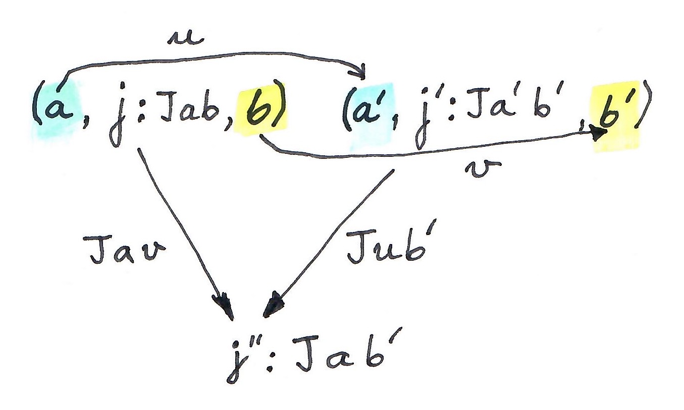
Given a profunctor $J \colon A^{op} \times B \to Set$ , an object in the category of elements is a triple $(a, j, b)$ . We interpret $j \in J \langle a, b \rangle$ as a witness that $a$ is related to $b$ .

A morphism in the category of elements between $(a, j, b)$ and $(a', j', b')$ is a pair of morphisms $(u \colon a \to a', v \colon b \to b')$ such that:

$J \langle a, v \rangle \,j = J \langle u, b' \rangle \, j'$

Here $J \langle a, v \rangle = J \langle id_a, v \rangle$ is the whiskering, or the lifting of a pair of morphisms, one of which is an identity, by the profunctor $J$ ; and similarly for $J \langle u, b' \rangle$ . We want the result, in both cases, to give us the same element of $J \langle a, b' \rangle$ — the witness that $a$ is related to $b'$ .

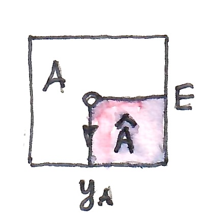
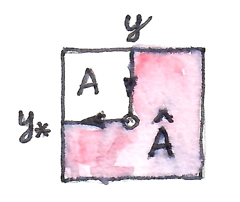
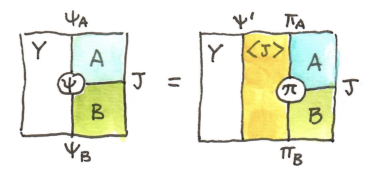
The analog of a graph of a profunctor in a double category is called a tabulation. A tabulation of a horizontal arrow $J \colon A \to B$ is a 0-cell $\langle J \rangle$ equipped with two projections. Think of these projections as extracting the two objects from the triple that we used in the definition of a graph of a profunctor. Their relation to $J$ is illustrated by the following 2-cell:

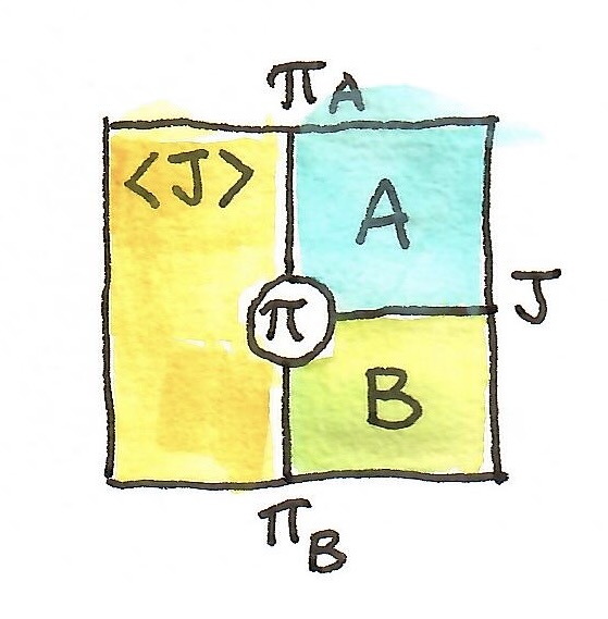
Let’s see how this works in $\mathbb{P}rof$ . Here we have a typical square that we’ve seen before, except that there is an invisible identity profunctor on the left — a hom-functor in the category $\langle J \rangle$ . The square tells us that for every morphism in $\langle J \rangle$ we can find a corresponding element of the profunctor $J$

Let’s pick two objects (triples) in $\langle J \rangle$ and a hom set between them:

$\langle J \rangle ((a, j, b), (a', j', b'))$

An element of this hom-set is a pair of morphisms $(u \colon a \to a', v \colon b \to b')$ . The 2-cell $\pi$ is a natural transformation whose components are:

$\pi_{(a, j, b)(a', j', b')} \colon \langle J \rangle ((a, j, b), (a', j', b')) \to J ( \pi_A (a, j, b), \pi_B (a', j', b'))$

Using our definitions, the argument of this mapping is a pair $(u, v)$ and the result is an element of the set $J(a, b')$ .

The mapping can be instantiated either by the lifting (whiskering) of $u$ or $v$ , both leading to the same result.

In a double category, we define a tabulation using its universal property. Just like a categorical product is universally defined by its mapping-in condition, so is a tabulation. However, since we are now working in a double category, besides the 1-dimensional mapping-in condition, we also need a 2-dimensional condition for 2-cells.

1-dimensional condition

What makes the projections projections is the mapping-in condition from some arbitrary 0-cell $X$ . We postulate that for any 0-cell $X$ that is equipped with two 1-cells $\phi_A$ and $\phi_B$ there is a unique factorization through the universal 2-cell $\pi$ :

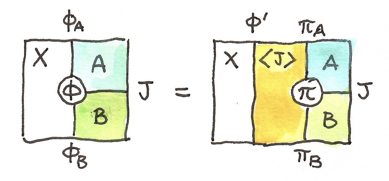
In $\mathbb{P}rof$ , these 2-cells correspond to natural transformations:

$\phi_{x, x'} \colon X(x, x') \to J(\phi_A x, \phi_B x')$

$(\pi \circ id_{\phi'})_{x, x'} \colon X(x, x') \to J (\pi_A (\phi' x), \pi_B (\phi' x'))$

We can then define $\phi'$ , on objects, as:

$\phi' x = (\phi_A x, \phi_{x, x} id_x, \phi_B x)$

and acting on a morphism $f \colon x \to x'$ , as $(\phi_A f, \phi_B f)$ .

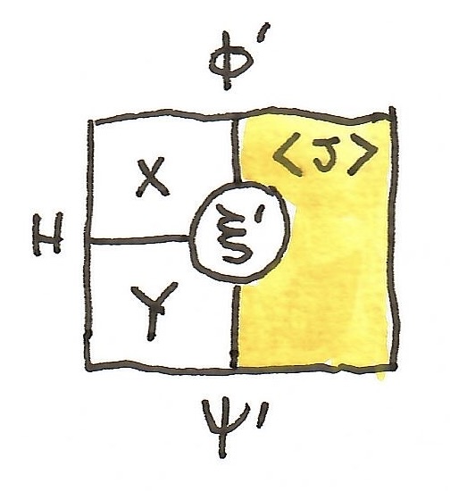
To summarize, the 1-dimensional condition lets us construct a vertical mapping $\phi' \colon X \to \langle J \rangle$ . All we have to provide is two vertical arrows and a 2-cell. But to complete the picture, we should be able to construct a 2-cell from another horizontal 1-cell, $H$ . For that we need a 2-dimensional universal condition.

2-dimensional condition

A 2-dimensional condition combines two instances of the one-dimensional condition. The second instance is another 0-cell $Y$ together with a projection $\psi$ , such that:

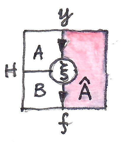
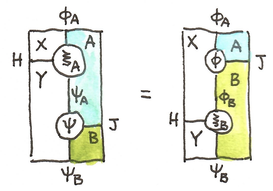
Using these two instances, we want to construct a mapping out of a horizontal 1-cell $H$ . There are two ways of combining these two instances on top of each other, and we postulate that the resulting 2-cells be equal:

In $\mathbb{P}rof$ , this corresponds to two natural transformations:

$\xi_{A\, x, y} \colon H(x, y) \to A(\phi_A x, \psi_A y)$
$\xi_{B\, x, y} \colon H(x, y) \to B(\phi_B x, \psi_B y)$

with the two composites equal:

$H(x, y) \to \int^{y'} A (\phi_A x, \psi_A y') \times J(\psi_A y', \psi_B y)$
$H(x, y) \to \int^{x'} J (\phi_A x, \phi_B x') \times B(\phi_B x', \psi_B y)$

The two-dimensional universal condition then statest that there is a unique 2-cell $\xi'$ :

such that both $\xi_A$ and $\xi_B$ factor through it. Here’s the first factorization:

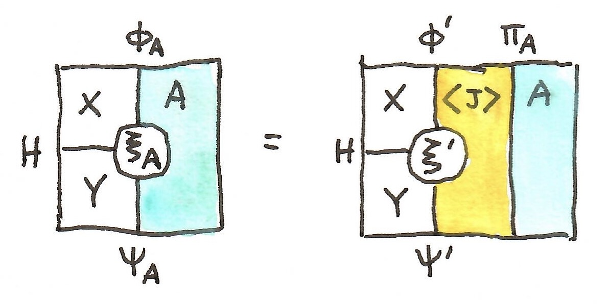
In $\mathbb{P}rof$ , $\xi'$ is a natural transformation with a component:

$\xi'_{x, y} \colon H(x, y) \to \langle J \rangle (\phi' x, \psi' y)$

Substituting our definitions of $\phi'$ and $\psi'$ , we get as the target a pair of morphisms:

$(u \colon \phi_A x \to \psi_A y, v \colon \phi_B x \to \psi_B y)$

Given $h \in H (x, y)$ , we can construct such a pair as:

$( \xi_{A\, x, y} h, \xi_{B\, x, y} h)$

When followed by $id_{\pi_A}$ this produces $\xi_{A x, y}$ thus satisfying the 2-dimensional universal condition. The constraints on $\xi_A$ and $\xi_B$ ensure that the pair of morphisms is indeed a proper morphism in $\langle J \rangle$ .

The same argument works when we replace $A$ with $B$ .

From the practical point of view, the 2-dimensional condition lets us construct a mapping (a 2-cell) $\xi'$ from a horizontal 1-cell $H$ to $\langle J \rangle$ using a pair of mappings into $A$ and $B$ satisfying coherency conditions.

The advantage of the universal construction is that it avoids talking about individual sets or, for that matter, about the category of sets. It thus works out of the box for enriched profunctors and other exotic embodiments of double categories.

May 18, 2026

Bending, Yanking, and Cartesian Squares in Double Categories

Posted by Bartosz Milewski under Category Theory | Tags: Category Theory, Double Categories, Proarrow Equipment, Profunctor Equipment, Profunctors, String Diagrams |
Leave a Comment

Previously: Profunctor Equipment in Haskell.

The major advantage of string diagrams is that they provide surprisingly natural language for complex diagram manipulations. The fact that two traditional diagrams are equal can be often described as a permission to bend, yank, or pinch strings in particular ways. They provide visual and often tactile clues to our senses. This is even more helpful in the context of double categories and equipments.

Yanking

Consider the definition of a companion from the previous installment. It’s a horizontal arrow $B(f, 1)$ that is somehow related to a vertical arrow $f \colon A \to B$ . There are two 2-cells that illustrate this relation, but it’s not clear what their meaning is or how to use them.

It’s only when you start composing these cells that the computational aspect of companions emerges. The first condition is that the horizontal composite result in the identity $\eta \epsilon = id_f$ . Diagrammatically, we have:

You can visualize this as yanking the ends of the two arrows and letting the beads fall down.

The same trick can be done with vertical composition. The equation, $\epsilon \odot \eta = id_{B(1, f)}$ , is illustrated by the following diagrams:

This time we yank the arrows horizontally.

The two equalites for the conjoint arrows have analogous graphical interpretation resulting it this general rule that is valid in any proarrow equipment:

Any zig-zag in which the arrows flow in one direction and vertical arrows point downwards can be yanked.

The Spider Lemma

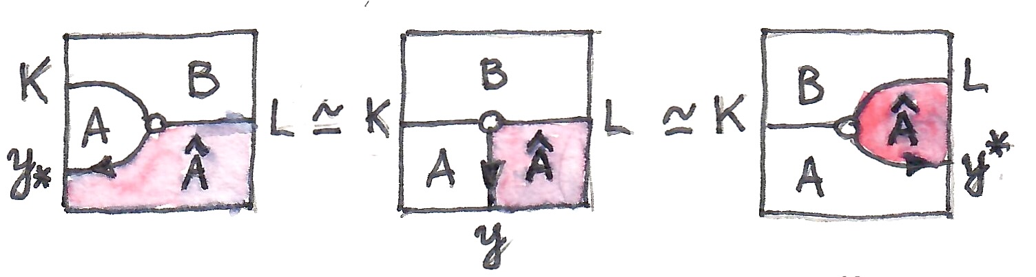
The yanking identities let us prove a very powerful lemma, which lets us bend arrows in many diagrams. The so called spider lemma states that the two diagrams below are isomorphic.

To prove it, we fist etablish two mappings: To get from the left diagram to the right one, we top it (vertically precompose) with the unit of the conjoint and the unit of the companion. This bends the arrows $f_1$ and $f_3$ and turns them into $A_1(1, f_1)$ and $A_3(f_3, 1)$ . Then we shove the two counits below it (vertically postcompose), to bend the arrows $g_1$ and $g_3$ .

To get from the right diagram to the left one, we do the analogous trick with horizontal pre/post composition. Finally, we prove that the two mappings are the inverse of each other by composing them and applying the yanking identities.

This is the spider lemma in its full glory, but we often specialize it to situations when one or more vertical arrows are identities. Then it lets us bend the remaining arrows.

Cartesian Squares

The workhorse of category theory is the universal construction. You define a new gadget by specifying its shape, and then pick the one through which all those shapes uniquely factor through. This is, for instance, how a categorical product is defined: The shape is a span with two fixed objects at its ends and a central object with arrows towards those objects. The product is the span through which all other spans factor through.

The same idea works in a double category, except that now we want to view it through string diagrams. We’ll illustrate it with the definition of a cartesian square.

Given a horizontal arrow $J$ and two vertical arrows $f$ and $g$ , a cartesian square defines a horizontal arrow $H = J(f, g)$ also called a restriction of $J$ along $f$ and $g$ . In the profunctor equipment $\mathbb{P}rof$ , this restriction is given by the hom-functor:

$\langle a, c \rangle \mapsto J(f a, g c)$

Since we want to avoid mentioning hom-sets, we’ll use a universal construction instead. Here’s the shape we are going to study:

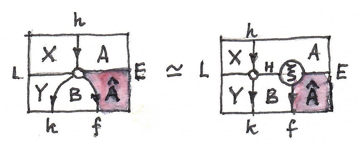
We are given four 0-cells (the four areas), two vertical 1-cells $f$ and $g$ , and one horizontal cell $J$ . We want to find the universal one of $H$ and $\alpha$ . To this end we replace $H$ with a generic horizontal arrow $L \colon X \to Y$ , together with two new vertical arrows $h$ and $k$ that, just like $H$ and $\alpha$ before, are equipped with a 2-cell $\psi$ (see the left diagram below).

The universal condition states that any such shape can be uniquely factored out through the cartesian square $\alpha$ (see the right diagram below).

Visually, we are splitting the bead representing $\psi$ into two separate beads, the right one being the universal one. Or you may interpret it, right to left, as pinching together the two beads into one.

Most universal constructions in a double category look like this. You may easily figure out the definition of the opcartesian square by extending it on the right instead of on the left.

In $\mathbb{P}rof$ , this universal condition is a tautology, but in other double categories it may have computational meaning. It can be used, for instance, to compute a 2-cell $\psi'$ from $L$ to $J(f, g)$ over a pair of 1-cells $(h, k)$ , given the corresponding cartesian square $\alpha$ . All we need is to find a suitable $\psi$ from $L$ to $J$ over the composite $(f \circ h, g \circ k)$ .

May 16, 2026

Profunctor Equipment in Haskell

Posted by Bartosz Milewski under Category Theory, Haskell, Programming | Tags: Category Theory, Haskell, Profunctor Equipment |
[2] Comments

Previously: Profunctor Equipment.

To make things more palatable for programmers, I decided to provide a toy implementation of some of the equipments in Haskell. The advantage of this encoding is that it can be verified by the compiler, and I still trust the compiler more than I trust the AI.

A more adequate implementation would require a full-blown dependently typed language, but if we restrict ourselves to just a single category and work only with endo-functors and endo-profunctors, we can get at least some intuitions. If you want to see a more elaborate version, see the proarrows library by Sjoerd Visscher.

The only 0-cell I’ll be using is the Haskell category of types and functions. For vertical 1-cells I’ll use the standard library implementation of Functor, and for horizontal ones I’ll use Profunctor.

A 2-cell in $\mathbb{P}rof$ :

is implemented as a natural transformation:

type Cell f g h j = forall a c . h a c -> j (f a) (g c)

The forall serves as a universal quantifier.

The horizontal composition of such cells is given by:

hcomp :: (Functor f, Functor f', Functor g, Functor g'
         , Profunctor h, Profunctor j, Profunctor k) =>
    Cell f g h j -> Cell f' g' j k 
                 -> Cell (Compose f' f) (Compose g' g) h k
hcomp fg_hj fg_jk hac = dimap getCompose Compose $ fg_jk (fg_hj hac)

I used the library definition of functor composition:

newtype Compose f g a = Compose { getCompose :: f (g a) }

Vertical composition of cells uses a more elaborate profunctor composition:

vcomp :: (Functor f, Functor g, Functor h
         , Profunctor p, Profunctor q, Profunctor r, Profunctor s) =>
    Cell f g p r -> Cell g h q s 
                 -> Cell f h (Procompose q p) (Procompose s r)
vcomp fg_pr gh_qs (Procompose qxc pax) 
    = Procompose (gh_qs qxc) (fg_pr pax)

Profunctor composition is defined using a coend. In Haskell, we implement a coend:

$\int^x P \langle x, c\rangle \times Q \langle d, x \rangle$

as an existential type:

data Procompose p q d c where
  Procompose :: p x c -> q d x -> Procompose p q d c

Here, x is a type that’s not in the argument list, so it’s interpreted using the existential counterpart of forall.

This is the horizontal unit cell:

type Hunit p = Cell Identity Identity p p

hUnit :: Profunctor p => Hunit p
hUnit = dimap runIdentity Identity

and here’s its vertical counterpart:

type Vunit f a b = Cell f f (->) (->)

vUnit :: Functor f => Vunit f a b
vUnit = fmap

I used the library implementation of the Identity functor, and the type constructor (->) for the hom-profunctor–the unit of profunctor composition. The unit laws are satisfied up to isomorphism.

The companion and the conjoint are synonyms of the library types Costar and Star:

newtype Star f d c   = Star   { runStar   :: d -> f c }
newtype Costar f d c = Costar { runCostar :: f d -> c }

type Companion f d c = Costar f d c
type Conjoint f d c  = Star f d c

The companion unit and counit cells:

are given by, respectively:

type CompUnit f   = Cell Identity f (->) (Costar f)

compUnit :: Functor f => CompUnit f
compUnit h = Costar (fmap (h . runIdentity))

and

type CompCoUnit f = Cell f Identity (Costar f) (->)

compCoUnit :: Functor f => CompCoUnit f 
compCoUnit (Costar h) = Identity . h

Similarly for the conjoint:

type ConjUnit f   = Cell f Identity (->) (Star f)

conjUnit :: Functor f => ConjUnit f 
conjUnit h = Star  (fmap (Identity . h))

and:

type ConjCoUnit f = Cell Identity f (Star f) (->)

conjCoUnit :: Functor f => ConjCoUnit f 
conjCoUnit (Star h) = h . runIdentity

More advanced constructions would require the definition of categories internal to Hask and the use of dependent types.

Haskell code is available here.

April 24, 2026

Profunctor Equipment

Posted by Bartosz Milewski under Category Theory | Tags: Category Theory, Companion, Conjoint, Double Category, Proarrow Equipment, Profunctors, String Diagrams |
1 Comment

The fundamental premise of category theory is that it’s possible to fully capture the nature of objects by describing their interactions with other objects of the same type. Those interactions are encoded using morphisms: arrows between objects.

What about categories themselves? We define a category by describing its internals: objects and arrows. But true to the categorical credo, we should be able to capture the essence of a category by describing its interactions with other categories. (Small) categories are objects in the category of categories $Cat$ , with functors as morphisms.

In fact $Cat$ has even more structure: functors between any two categories form a functor category, with natural transformations as morphisms. This makes $Cat$ a 2-category, with categories as 0-cells, functors as 1-cells, and natural transformations as 2-cells.

With this much structure, we can define a lot of categorical constructions. In particular, we can define adjunctions as pairs of functors equipped with the unit and counit natural transformations. We can also define monads as endofunctors equipped with the unit and multiplication natural transformations, and so on.

However, there are some categorical constructions that force us to look at the internals of categories. In particular, anything that involves representable functors cannot be defined without talking about hom-sets, which are internal to categories. In particular there are things like (weighted) limits or pointwise Kan extensions that rely on representability.

We somehow need to incorporate the information about hom-sets into the fabric of of the 2-category $Cat$ . At the minimum, we need to identify the hom-functors:

$C(-, =) \colon C^{op} \times C \to Set$

Such functors of mixed variance are called profunctors and, in general, they can go between different categories, as in $P \colon C^{op} \times D \to Set$ . In fact, profunctors can be considered arrows in the category $Prof$ . Not only that, $Prof$ is itself a bicategory, whose 0-cells are (small) categories, 1-cells are profunctors, and 2-cells are natural transformations between profunctors. Composition of profunctors is defined using the coend formula:

$(P \odot Q)\langle c, e \rangle = \int^{d \colon D} P \langle c, d \rangle \times Q \langle d, e \rangle$

What is important is that the hom-functor $C(-, =)$ is the identity profunctor with respect to this composition. It means that we have a way of talking about hom-sets and representables without peeking inside individual categories.

The usual categorical laws, associativity and identity, are only satisfied up to isomorphism (that is up to invertible 2-cells), hence $Prof$ is called a bicategory and not a 2-category, whose laws are satisfied on the nose.

These two categories, the 2-category $Cat$ and the bicategory $Prof$ can be combined into a single double category, which we’ll call $\mathbb{P}rof$ . The 0-cells are the usual categories; but now we have two kinds of arrows: the vertical ones are functors, and the horizontal ones are profunctors. What glues them together are the 2-cells.

Here’s a 2-cell that combines two (vertical) functors $f \colon A \to B$ and $g \colon C \to D$ with two (horizontal) profunctors $H \colon A \to C$ and $J \colon B \to D$ .

In our double category $\mathbb{P}rof$ , this 2-cell is implemented as a natural transformation, whose component at the pair of objects $\langle a, c \rangle$ is a function:

$\alpha_{\langle a, c \rangle} \colon H \langle a, c \rangle \to J \langle f a, g c \rangle$

It’s a member of the set of natural transformations, which can be written as an end:

$\int_{a c} Set(H \langle a, c \rangle, J \langle f a, g c \rangle)$

The profunctor $J \langle f a, g c \rangle$ is sometimes called the restriction of $J$ along $f$ and $g$ .

In an abstract double category, a 2-cell is just something that says that the particular four arrows in this configuration are related.

The same diagram can be transformed into a string diagram. Here, the 0-cells are the four areas, 1-cells form boundaries between those areas, and a 2-cell is a node connecting the four subdivisions:

We encode identity 1-cells in string diagrams by simply omitting the corresponding lines/arrows.

2-cells can be composed both horizontally and vertically by gluing them along identical edges.

In $\mathbb{P}rof$ , horizontal composition of 2-cells corresponds to the (vertical) composition of natural transformations between profunctors (we’ll write this composition as a juxtaposition, as in $\alpha \beta$ , in diagram order).

The identity 2-cell at a profunctor $P$ is just an identity natural transformation:

Vertical gluing of string diagrams results is a natural transformation between composite profunctors. For instance this diagram:

is a composition of two natural transformation:

$\alpha_{\langle a, c \rangle} \colon P \langle a, c \rangle \to R \langle f a, g c \rangle$
$\beta_{\langle c, e \rangle} \colon Q \langle c, e \rangle \to S \langle g c, h e \rangle$

whose component is a function:

$(\beta \odot \alpha)_{\langle a, e \rangle} \colon \int^c P\langle a, c \rangle \times Q \langle c, e \rangle \to \int^{c'} R \langle f a, g c' \rangle \times S \langle g c', h e \rangle$

By co-continuity of the coend, this is isomorphic to:

$\int_c \big(P\langle a, c \rangle \times Q \langle c, e \rangle \to \int^{c'} R \langle f a, g c' \rangle \times S \langle g c', h e \rangle \big)$

and is implemented by composing the product $\alpha_{\langle a, c \rangle} \times \beta_{\langle c, e \rangle}$ with the appropriate injection into the coend.

The unit of vertical composition at a functor $f$ in $\mathbb{P}rof$ is a 2-cell:

which is a natural transformation $A(a, a') \to B(f a, f a')$ implementing the functoriality of $f$ .

Companion and Conjoint

Given a functor $f \colon A \to B$ we can construct two representable profunctors, the companion and the conjoint.

The companion is denoted by $B(f, 1)$ . In $\mathbb{P}rof$ , it is the profunctor generated by the following hom-functor:

$\langle a, b \rangle \mapsto B (f a, b )$

A conjoint, which is denoted by $B(1, f)$ , is defined in $\mathbb{P}rof$ as:

$\langle b, a \rangle \mapsto B (b, f a)$

Notice that these two horizontal arrows go in opposite directions. The companion goes from $A$ to $B$ (the same as $f$ ), and the conjoint goes from $B$ to $A$ . Later we’ll see that they form an adjunction.

In these definitions we have used the hom-sets explicitly, something we were trying to avoid. We should therefore try to define the companions and the conjoints abstractly by listing their properties.

Companion

In a string diagram, the companion of a vertical arrow $f \colon A \to B$ is represented by a left-pointing horizontal arrow:

It is equipped with two 2-cells called the unit and the counit (the subscript $p$ stands for comPanion):

Indeed, using the rules for reading string diagrams in $\mathbb{P}rof$ , the unit corresponds to a natural transformation:

$\eta_{\langle a, a' \rangle} \colon A (a, a') \to B (f a, f a' )$

which just expresses the functoriality of $f$ . The (invisible) horizontal line on the left stands for the identity profunctor $A(a, a')$ .

The counit in $\mathbb{P}rof$ :

$\epsilon_{\langle a, b \rangle} \colon B (f a, b) \to B (f a, b)$

is trivially instantiated by the identity natural transformation.

There are two ways we can compose these two 2-cells. Both of them should result in some kind of identities. For instance, this is the horizontal composition:

$\eta \epsilon = id_f$

where $id_f$ is the identity at $f$ which, in $\mathbb{P}rof$ is a functorial action of $f$ on the hom-set.

Similarly, vertical composition gives us:

$\epsilon \odot \eta = id_{B(f, 1)}$

Conjoint

The conjoint of $f \colon A \to B$ is represented by the right-pointing horizontal arrow:

In $\mathbb{P}rof$ , the conjoint is the representable profunctor: $\langle b, b' \rangle \mapsto B(b, f b')$

The conjoint is related to the original functor by its unit and counit 2-cells:

(here, the subscript $j$ stands for conJoint). Their two compositions produce identity 2-cells:

$\eta \epsilon = id_f$
$\eta \odot \epsilon = id_{B(1, f)}$

Adjunction

We can also compose units with units and counits with counits by connecting the functor arrows:

These diagrams can be interpreted as the unit and counit of the adjunction $B(1, f) \dashv B(f, 1)$ :

$\eta \colon id_A \to B(f, 1) \odot B(1, f)$

$\epsilon \colon B(1, f) \odot B(f, 1) \to id_B$

In $Prof$ , the profunctor composition is given by the coend, so we get, for the unit:

$\eta \colon A(a, a') \to \int^b B(f a, b) \times B(b, f a')$

We use the Yoneda reduction to eliminate the coend:

$\int^b B(f a, b) \times B(b, f a') \cong B(f a, f a')$

The unit is then instantiated by the functoriality of $f$ .

The counit is:

$\int^a B(b, f a) \times B(fa, b') \to B(b, b')$

By co-continuity of the coend, this is isomorphic to:

$\int_a \big(B(b, f a) \times B(fa, b') \to B(b, b')\big)$

which is inhabited by the composition of hom-sets.

The Big Picture

We’ve seen how to combine the 2-category $Cat$ with the bicategory $Prof$ into one double category $\mathbb{P}rof$ . In this double category every vertical arrow has a horizontal companion and every companion has a conjoint. A double category with this kind of structure is called a proarrow equipment. It has just enough structure to define abstractly such categorical constructions as weighted limits or pointwise Kan extensions. We can then apply those constructions to other double categories, without having to repeat ourselves.

One immediate application is to enriched categories and enriched profunctors, which form a proarrow equipment $\mathbb{V}\text{-Cat}$ . Or we can consider a simpler case of the double category of sets and relations. We can also add more structure to the categories in question, for instance by considering monoidal categories; or even go meta, and study the double category of (weak) double categories $\mathbb{D}bl$ .

March 10, 2026

The Axiom of Univalence

Posted by Bartosz Milewski under Homotopy, Homotopy Type Theory | Tags: Homotopy, HoTT, mathematics |
[2] Comments

Previously: Modeling Identity Types.

On first viewing, the identity type seems odd. Does it make sense to replace the traditional yes/no equality predicate with an elaborate type of equality proofs? In fact the father or modern type theory Martin Löf had his doubts, and initially tried to reflect all identity proofs into more basic judgmental or definitional equalities. This turned out to be too restrictive for many applications.

Still, some modern theorem provers like Lean impose the uniqueness of identity proofs (UIP) condition as an axiom. This so called axiom K states that reflexivity:

$\text{refl} (a) : \text{Id}_A (a, a)$

is the only possible proof of equality. Two things are equal if they are the same thing, otherwise they’re not. This works for most common data types.

Universes

There is, however, a much more interesting use case for non-trivial identity types. This happens when we apply equality to types themselves.

Since type theory is all about types, the question naturally arises, what is a type of a type? In Haskell, we call it a kind and denote as Type (or *, in legacy code).

In type theory we say that types form a universe. In Agda, the lowest such universe, $U_0$ , is called Type l-zero (level zero), often abbreviated to Type. Of course, this begs the next question, what is the type of Type? Well, Type is a member of the next universe $U_1$ , and so on, ad infinitum.

But if Type is a type then, like all types, it must be equipped with its own identity type. In other words, we should be albe to compare types for equality. The most obvious choice would be to say that two types are equal if they are isomorphic. We define an isomorphism as a pair of functions that are the inverse of each other. This makes perfect sense for sets, but we don’t want to treat types as sets. Types have more structure: every type comes equipped with its own identity type.

Equivalences

We’ve seen before that to model identity types we may look at homotopy theory. We model types as topological spaces and equality as continuous paths between points. The notion of isomorphism is too strong for comparing such spaces. What we need is an equivalence, which is an isomorphism modulo equality.

Indeed, we don’t need the round trip to land us exactly where we started — it’s enough that we land at a point that is equal to the original point. Here, equal means: there is a path that connects these two points. And once we have loosened the definition of what an inverse is, there is no reason to insist that the right inverse be the same as the left inverse. We can as well use two different functions, $g$ and $h$ .

Thus a function $f \colon A \to B$ is called an equivalence iff:

there exists a function $g \colon B \to A$ such that the composite $f \circ g \sim id_B\;$ , that is $\forall b \colon B . \; f (g\, b) =_B b$
there exists a function $h \colon B \to A$ such that the composite $h \circ f \sim id_A$ , that is $\forall a \colon A . \; h (f \, a) =_A a$ .

If such functions exist, we say that $A$ is equivalent to $B$ , $A \simeq B$ .

Univalence

Equivalence is the only relation between types that behaves exactly like equality. Can we use it to define equality of types? This is what Vladimir Voevodsky postulated as the axiom of univalence.

For any $A$ and $B$ in a universe $U$ , we postulate that:

$(A =_U B) \simeq (A \simeq B)$

in other words, equality is equivalent to equivalence.

Equivalences are much easier to prove than equalities. However, without univalence, they don’t satisfy the rule of substitution of equals for equals. This rule formulated by Leibniz reads: “Two terms are the same if one can be substituted for the other without altering the truth of any statement.”

In Martin Löf type theory it’s impossible to define a predicate that would distinguish between equivalent types. This is why imposing the axiom of univalence to extend type theory makes perfect sense.

Mathematician often apply the substitution rule to terms that are isomorphic rather than equal, essentially leaving the proof of the validity of a substitution as an “exercise to the reader.” Univalence legitimizes this practice and leads to substantial simplification of many mathematical proofs.

However, just like with isomorphisms, there may be several equivalences between two types. In fact, a type can be equivalent to itself in more than one way. For instance, not is a non-trivial equivalence for Bool — it’s clearly different from id. By univalence, such different equivalences introduce different equalities. Uniqueness of identity proofs is thus incompatible with univalence.

Higher Inductive Types

If identity is a type like any other, then we may use it to define types that contain their own proofs of identity. Such types are called higher inductive types. The simplest example is the circle, which you may think of as a singleton $\text{base}$ plus a proof $\text{loop}$ that $\text{base}$ is equal to itself. In Agda, which is a dependently typed language, this translates to:

			
data S¹ : Type where
  base : S¹
  loop : base ≡ base

Here, base ≡ base denotes the type $\text{Id}_{S^1} (\text{base}, \text{base})$ .

This definition is somewhat similar to, say, the definition of a boolean type:

			
data Bool : Type where
  true  : Bool
  false : Bool

except that, in the definition of the circle, the type of the second component depends on the value of the first component. This definition introduces explicitly an element of the identity type, $\text{loop}$ , that is not $\text{refl}$ . It is therefore incompatible with axiom K.

Higher inductive types can be used to prove theorems in topological homotopy. Such proofs would normally involve topology, but in HoTT they are just statements about types. They can be formalized using theorem provers, like Agda.

I’m grateful to Thorsten Altenkirch for valuable comments on the draft of this post.

October 18, 2025

Modeling Identity Types

Posted by Bartosz Milewski under Category Theory, Homotopy, Homotopy Type Theory, Topology | Tags: Category Theory, Homotopy, HoTT, Identity Type, Topology |
1 Comment

Previously: Identity Types.

Let me first explain why the naive categorical model of dependent types doesn’t work very well for identity types. The problem is that, in such a model, any arrow can be considered a fibration, and therefore interpreted as a dependent type. In our definition of path induction, with an arrow $d$ that makes the outer square commute, there are no additional constraints on $\rho$ :

So we are free to substitute $\text{refl} \colon A \to \text{Id}_A$ for $\rho$ , and use the identity for $d$ :

We are guaranteed that there is a unique $J$ that makes the two triangles commute. But these commutation conditions tell us that $J$ is the inverse of $\text{refl}$ and, consequently, $\text{Id}_A$ is isomorphic to $A$ . It means that there are no paths in $\text{Id}_A$ other than those given by reflexivity.

This is not satisfactory from the point of homotopy type theory, since the existence of non-trivial paths is necessary to make sense of things like higher inductive types (HITs) or univalence. If we want to model dependent types as fibrations, we cannot allow $\text{refl}$ to be a fibration. Thus we need a more restrictive model in which not all mappings are fibrations.

The solution is to apply the lessons from topology, in particular homotopy. Recall that maps between topological spaces can be characterized as fibrations, cofibrations, and homotopy equivalences. There usually are overlaps between these three categories.

A fibration that is also an equivalence is called a trivial fibration or an acyclic fibration. Similarly, we have trivial (acyclic) cofibrations. We’ve also seen that, roughly speaking, cofibrations generalize injections. So, if we want a non-trivial model of identity types, it makes sense to model $\text{refl}$ as a cofibration. We want different values $a \colon A$ to be mapped to different “paths” $\text{refl}(a) \colon \text{Id}_A$ , and we’d also like to have some non-trivial paths left over to play with.

We know what a path is in a topological space $A$ : it’s a continuous mapping from a unit interval, $\gamma \colon I \to A$ . In a cartesian category with weak equivalences, we can use an abstract definition of the object representing the space of all paths in $A$ . A path space object $P_A$ is an object that factorizes the diagonal morphism $\Delta = \pi \circ s$ , such that $s$ is a weak equivalence.

In a category that supports a factorization system, we can tighten this definition by requiring that $\pi$ be a fibration, defining a good path object; and $s$ be a cofibration (therefore a trivial cofibration) defining a very good path object.

The intuition behind this diagram is that $\pi$ produces the start and the end of a path, and $s$ sends a point to a constant path.

Compare this with the diagram that illustrates the introduction rule for the identity type:

We want $\text{refl}$ to be a trivial cofibration, that is a cofibration that’s a weak homotopy equivalence. Weak equivalence let us shrink all paths. Imagine a path as a rubber band. We fix one end and of the path and let the other end slide all the way back until the path becomes constant. (In the compact/open topology of $P_A$ , this works also for closed loops.)

Thus the existence of very good path objects takes care of the introduction rule for identity types.

The elimination rule is harder to wrap our minds around. How is it possible that any mapping that is defined on trivial paths, which are given by $\text{refl}$ over the diagonal of $A \times A$ , can be uniquely extended to all paths?

We might take a hint from complex analysis, where we can uniquely define analytic continuations of real function.

In topology, our continuations are restricted by continuity. When you are lifting a path in $A$ , you might not have much choice as to which value of type $D(a)$ to pick next. In fact, there might be only one value available to you — the “closest one” in the direction you’re going. To choose any other value, you’d have to “jump,” which would break continuity.

You can visualize building $J(a, b, p)$ by growing it from its initial value $J(a, a, \text{refl}(a)) = d(a)$ . You gradually extend it above the path $p$ until you reach the point directly above $b$ . (In fact, this is the rough idea behind cubical type theory.)

A more abstract way of putting it is that identity types are path spaces in some factorization system, and dependent types over them are fibrations that satisfy the lifting property. Any path from $a$ to $b$ in $\text{Id}_A$ has a unique lifting $J$ in $D$ that starts at $d(a)$ .

This is exactly the property illustrated by the lifting diaram, in which paths are elements of the identity type $\text{Id}_A$ :

This time $\text{refl}$ is not a fibration.

The general framework, in which to build models of homotopy type theory is called a Quillen model category, which was originally used to model homotopies in topological spaces. It can be described as a weak factorization system, in which any morphism can be written as a trivial cofibration followed by a fibration. It must satisfy the unique lifting property for any square in which $i$ is a cofibration, $p$ is a fibration, and one of them is a weak equivalence:

The full definition of a model category has more moving parts, but this is the gist of it.

We model dependent types as fibrations in a model category. We construct path objects as factorizations of the diagonal, and this lets us define non-trivial identity types.

One of the consequences of the fact that there could be multiple identity paths between two points is that we can, in turn, compare these paths for equality. There is, for instance, an identity type of identity types $\text{Id}_{\text{Id}_A(a, b)}$ . Such iterated types correspond to higher homotopies: paths between paths, and so on, ad infinitum. The structure that arises is called a weak infinity groupoid. It’s a category in which every morphism has an inverse (just follow the same path backwards), and category laws (identity or associativity) are satisifed up to higher morphisms (higher homotopies).

Monoidal functors redux

Tambara modules

Tambara Equipment

Free Tambara and Optics

Internalizing monoidal actions

Internal monoid

Monoidal Category

Actegory

Monoidal Functors

Right Kan extensions in Haskell

Left Kan extensions

Left Kan extensions in Haskell

Right Kan extensions

Universal arrows

Left Kan extensions

1-dimensional condition

2-dimensional condition

Yanking

The Spider Lemma

Cartesian Squares

Companion and Conjoint

Companion

Conjoint

Adjunction

The Big Picture

Universes

Equivalences

Univalence

Higher Inductive Types

Top Posts

License

Blogroll

Follow Me

Archives