The series of posts about so called benign data races stirred a lot of controversy and led to numerous discussions at the startup I was working at called Corensic. Two bastions formed, one claiming that no data race was benign, and the other claiming that data races were essential for performance. Then it turned out that we couldn’t even agree on the definition of a data race. In particular, the C++11 definition seemed to deviate from the established notions.

What Is a Data Race Anyway?

First of all, let’s make sure we know what we’re talking about. In current usage a data race is synonymous with a low-level data race, as opposed to a high-level race that involves either multiple memory locations, or multiple accesses per thread. Everybody agrees on the meaning of data conflict, which is multiple threads accessing the same memory location, at least one of them through a write. But a data conflict is not necessarily a data race. In order for it to become a race, one more condition must be true: the access has to be “simultaneous.”

Unfortunately, simultaneity is not a well defined term in concurrent systems. Leslie Lamport was the first to observe that a distributed system follows the rules of Special Relativity, with no independent notion of simultaneity, rather than those of Galilean Mechanics, with its absolute time. So, really, what defines a data race is up to your notion of simultaneity.

Maybe it’s easier to define what isn’t, rather than what is, simultaneous? Indeed, if we can tell which event happened before another event, we can be sure that they weren’t simultaneous. Hence the use of the famous “happened before” relationship in defining data races. In Special Relativity this kind of relationship is established by the exchange of messages, which can travel no faster than the speed of light. The act of sending a message always happens before the act of receiving the same message. In concurrent programming this kind of connection is made using synchronizing actions. Hence an alternative definition of a data race: A memory conflict without intervening synchronization.

The simplest examples of synchronizing actions are the taking and the releasing of a lock. Imagine two threads executing this code:

  mutex.lock();
  x = x + 1;
  mutex.unlock();

In any actual execution, accesses to the shared variable x from the two threads will be separated by a synchronization. The happens-before (HB) arrow will always go from one thread releasing the lock to the other thread acquiring it. For instance in:

#	Thread 1	Thread 2
1		mutex.lock();
2		x = x + 1;
3		mutex.unlock();
4	mutex.lock();
5	x = x + 1;
6	mutex.unlock();

the HB arrow goes from 3 to 4, clearly separating the conflicting accesses in 2 and 5.

Notice the careful choice of words: “actual execution.” The following execution that contains a race can never happen, provided the mutex indeed guarantees mutual exclusion:

#	Thread 1	Thread 2
1		mutex.lock();
2	mutex.lock();
3	x = x + 1;	x = x + 1;
4		mutex.unlock();
5	mutex.unlock();

It turns out that the selection of possible executions plays an important role in the definition of a data race. In every memory model I know of, only sequentially consistent executions are tried in testing for data races. Notice that non-sequentially-consistent executions may actually happen, but they do not enter the data-race test.

In fact, most languages try to provide the so called DRF (Data Race Free) guarantee, which states that all executions of data-race-free programs are sequentially consistent. Don’t be alarmed by the apparent circularity of the argument: you start with sequentially consistent executions to prove data-race freedom and, if you don’t find any data races, you conclude that all executions are sequentially consistent. But if you do find a data race this way, then you know that non-sequentially-consistent executions are also possible.

As you can see, in order to define a data race you have to precisely define what you mean by “simultaneous,” or by “synchronization,” and you have to specify to which executions your definition may be applied.

The Java Memory Model

In Java, besides traditional mutexes that are accessed through “synchronized” methods, there is another synchronization device called a volatile variable. Any access to a volatile variable is considered a synchronization action. You can draw happens-before arrows not only between consecutive unlocks and locks of the same object, but also between consecutive accesses to a volatile variable. With this extension in mind, Java offers the the traditional DRF guarantee. The semantics of data-race free programs is well defined in terms of sequential consistency thus making every Java programmer happy.

But Java didn’t stop there, it also attempted to provide at least some modicum of semantics for programs with data races. The idea is noble–as long as programmers are human, they will write buggy programs. It’s easy to proclaim that any program with data races exhibits undefined behavior, but if this undefined behavior results in serious security loopholes, people get really nervous. So what the Java memory model guarantees on top of DRF is that the undefined behavior resulting from data races cannot lead to out-of-thin-air values appearing in your program (for instance, security credentials for an intruder).

It is now widely recognized that this attempt to define the semantics of data races has failed, and the Java memory model is broken (I’m citing Hans Boehm here).

The C++ Memory Model

Why is it so important to have a good definition of a data race? Is it because of the DRF guarantee? That seems to be the motivation behind the Java memory model. The absence of data races defines a subset of programs that are sequentially consistent and therefore have well-defined semantics. But these two properties: being sequentially consistent and having well-defined semantics are not necessarily the same. After all, Java tried (albeit unsuccessfully) to define semantics for non sequentially consistent programs.

So C++ chose a slightly different approach. The C++ memory model is based on partitioning all programs into three categories:

1. Sequentially consistent,
2. Non-sequentially consistent, but with defined semantics, and
3. Incorrect programs with undefined semantics

The first category is very similar to race-free Java programs. The place of Java volatile is taken by C++11 default atomic. The word “default” is crucial here, as we’ll see in a moment. Just like in Java, the DRF guarantee holds for those programs.

It’s the second category that’s causing all the controversy. It was introduced not so much for security as for performance reasons. Sequential consistency is expensive on most multiprocessors. This is why many C++ programmers currently resort to “benign” data races, even at the risk of undefined behavior. Hans Boehm’s paper, How to miscompile programs with “benign” data races, delivered a death blow to such approaches. He showed, example by example, how legitimate compiler optimizations may wreak havoc on programs with “benign” data races.

Fortunately, C++11 lets you relax sequential consistency in a controlled way, which combines high performance with the safety of well-defined (if complex) semantics. So the second category of C++ programs use atomic variables with relaxed memory ordering semantics. Here’s some typical syntax taken from my previous blog post:

std::atomic<int> owner = 0
...
owner.load(memory_order_relaxed);

And here’s the controversial part: According to the C++ memory model, relaxed memory operations, like the above load, don’t contribute to data races, even though they are not considered synchronization actions. Remember one of the versions of the definition of a data race: Conflicting actions without intervening synchronization? That definition doesn’t work any more.

The C++ Standard decided that only conflicts for which there is no defined semantics are called data races.

Notice that some forms of relaxed atomics may introduce synchronization. For instance, a write access with memory_order_release “happens before” another access with memory_order_acquire, if the latter follows the former in a particular execution (but not if they are reversed!).

Conclusion

What does it all mean for the C++11 programmer? It means that there no longer is an excuse for data races. If you need benign data races for performance, rewrite your code using weak atomics. Weak atomics give you the same kind of performance as benign data races but they have well defined semantics. Traditional “benign” races are likely to be broken by optimizing compilers or on tricky architectures. But if you use weak atomics, the compiler will apply whatever means necessary to enforce the correct semantics, and your program will always execute correctly. It will even naturally align atomic variables to avoid torn reads and writes.

What’s more, since C++11 has well defined memory semantics, compiler writers are no longer forced to be conservative with their optimizations. If the programmer doesn’t specifically mark shared variables as atomic, the compiler is free to optimize code as if it were single-threaded. So all those clever tricks with benign data races are no longer guaranteed to work, even on relatively simple architectures, like the x86. For instance, compiler is free to use your lossy counter or a binary flag for its own temporary storage, as long as it restores it back later. If other threads access those variables through racy code, they might see arbitrary values as part of the “undefined behavior.” You have been warned!
Follow @BartoszMilewski

This post is based on the talk I gave in Moscow, Russia, in February 2015 to an audience of C++ programmers.

Let’s agree on some preliminaries.

C++ is a low level programming language. It’s very close to the machine. C++ is engineering at its grittiest.

Category theory is the most abstract branch of mathematics. It’s very very high in the layers of abstraction. Category theory is mathematics at its highest.

So why have I decided to speak about category theory to C++ programmers? There are many reasons.

The main reason is that category theory captures the essence of programming. We can program at many levels, and if I ask somebody “What is programming?” most C++ programmers will probably say that it’s about telling the computer what to do. How to move bytes from memory to the processor, how to manipulate them, and so on.

But there is another view of programming and it’s related to the human side of programming. We are humans writing programs. We decide what to tell the computer to do.

We are solving problems. We are finding solutions to problems and translating them in the language that is understandable to the computer.

But what is problem solving? How do we, humans, approach problem solving? It was only a recent development in our evolution that we have acquired these fantastic brains of ours. For hundreds of millions of years not much was happening under the hood, and suddenly we got this brain, and we used this brain to help us chase animals, shoot arrows, find mates, organize hunting parties, and so on. It’s been going on for a few hundred thousand years. And suddenly the same brain is supposed to solve problems in software engineering.

So how do we approach problem solving? There is one general approach that we humans have developed for problem solving. We had to develop it because of the limitations of our brain, not because of the limitations of computers or our tools. Our brains have this relatively small cache memory, so when we’re dealing with a huge problem, we have to split it into smaller parts. We have to decompose bigger problems into smaller problems. And this is very human. This is what we do. We decompose, and then we attack each problem separately, find the solution; and once we have solutions to all the smaller problems, we recompose them.

So the essence of programming is composition.

If we want to be good programmers, we have to understand composition. And who knows more about composing than musicians? They are the original composers!

So let me show you an example. This is a piece by Johann Sebastian Bach. I’ll show you two versions of this composition. One is low level, and one is high level.

The low level is just sampled sound. These are bytes that approximate the waveform of the sound.

And this is the same piece in typical music notation.

Which one is easier to manipulate? Which one is easier to reason about? Obviously, the high level one!

Notice that, in the high level language, we use a lot of different abstractions that can be processed separately. We split the problem into smaller parts. We know that there are things called notes, and they can be reproduced, in this particular case, using violins. There are also some letters like E, A, B⁷: these are chords. They describe harmony. There is melody, there is harmony, there is the bass line.

Musicians, when they compose music, use higher level abstractions. These higher level abstractions are easier to manipulate, reason about, and modify when necessary.

And this is probably what Bach was hearing in his head.
 

 
And he chose to represent it using the high level language of musical notation.

Now, if you’re a rap musician, you work with samples, and you learn how to manipulate the low level description of music. It’s a very different process. It’s much closer to low-level C++ programming. We often do copy and paste, just like rap musicians. There’s nothing wrong with that, but sometimes we would like to be more like Bach.

So how do we approach this problem as programmers and not as musicians. We cannot use musical notation to lift ourselves to higher levels of abstraction. We have to use mathematics. And there is one particular branch of mathematics, category theory, that is exactly about composition. If programming is about composition, then this is what we should be looking at.

Category theory, in general, is not easy to learn, but the basic concepts of category theory are embarrassingly simple. So I will talk about some of those embarrassingly simple concepts from category theory, and then explain how to use them in programming in some weird ways that would probably not have occurred to you when you’re programming.

Categories

So what is this concept of a category? Two things: object and arrows between objects.

In category theory you don’t ask what these objects are. You call them objects, you give them names like A, B, C, D, etc., but you don’t ask what they are or what’s inside them. And then you have arrows that connect objects. Every arrow starts at some object and ends at some object. You can have many arrows going between two objects, or none whatsoever. Again, you don’t ask what these arrows are. You just give them names like f, g, h, etc.

And that’s it—that’s how you visualize a category: a bunch of objects and a bunch of arrows between them.

There are some operations on arrows and some laws that they have to obey, and they are also very simple.

Since composition is the essence of category theory (and of programming), we have to define composition in a category.

Whenever you have an arrow f going from object A to object B, here represented by two little piggies, and another arrow g going from object B to object C, there is an arrow called their composition, g ∘ f, that goes directly from object A to object C. We pronounce this “g after f.”

Composition is part of the definition of a category. Again, since we don’t know what these arrows are, we don’t ask what composition is. We just know that for any two composable arrows — such that the end of one coincides with the start of the other — there exists another arrow that’s their composition.

And this is exactly what we do when we solve problems. We find an arrow from A to B — that’s our subproblem. We find an arrow from B to C, that’s another subproblem. And then we compose them to get an arrow from A to C, and that’s a solution to our bigger problem. We can repeat this process, building larger and larger solutions by solving smaller problems and composing the solutions.

Notice that when we have three arrows to compose, there are two ways of doing that, depending on which pair we compose first. We don’t want composition to have history. We want to be able to say: This arrow is a composition of these three arrows: f after g after h, without having to use parentheses for grouping. That’s called associativity:

 (f ∘ g) ∘ h = f ∘ (g ∘ h)

Composition in a category must be associative.

And finally, every object has to have an identity arrow. It’s an arrow that goes from the object back to itself. You can have many arrows that loop back to the same object. But there is always one such loop for every object that is the identity with respect to composition.

It has the property that if you compose it with any other arrow that’s composable with it — meaning it either starts or ends at this object — you get that arrow back. It acts like multiplication by one. It’s an identity — it doesn’t change anything.

Monoid

I can immediately give you an example of a very simple category that I’m sure you know very well and have used all your adult life. It’s called a monoid. It’s another embarrassingly simple concept. It’s a category that has only one object. It may have lots of arrows, but all these arrows have to start at this object and end at this object, so they are all composable. You can compose any two arrows in this category to get another arrow. And there is one arrow that’s the identity. When composed with any other arrow it will give you back the same arrow.

There are some very simple examples of monoids. We have natural numbers with addition and zero. An arrow corresponds to adding a number. For instance, you will have an arrow that corresponds to adding 5. You compose it with an arrow that corresponds to adding 3, and you get an arrow that corresponds to adding 8. Identity arrow corresponds to adding zero.

Multiplication forms a monoid too. The identity arrow corresponds to multiplying by 1. The composition rule for these arrows is just a multiplication table.

Strings form another interesting monoid. An arrow corresponds to appending a particular string. Unit arrow appends an empty string. What’s interesting about this monoid is that it has no additional structure. In particular, it doesn’t have an inverse for any of its arrows. There are no “negative” strings. There is no anti-“world” string that, when appended to “Hello world”, would result in the string “Hello“.

In each of these monoids, you can think of the one object as being a set: a set of all numbers, or a set of all strings. But that’s just an aid to imagination. All information about the monoid is in the composition rules — the multiplication table for arrows.

In programming we encounter monoids all over the place. We just normally don’t call them that. But every time you have something like logging, gathering data, or auditing, you are using a monoid structure. You’re basically adding some information to a log, appending, or concatenating, so that’s a monoidal operation. And there is an identity log entry that you may use when you have nothing interesting to add.

Types and Functions

So monoid is one example, but there is something closer to our hearts as programmers, and that’s the category of types and functions. And the funny thing is that this category of types and functions is actually almost enough to do programming, and in functional languages that’s what people do. In C++ there is a little bit more noise, so it’s harder to abstract this part of programming, but we do have types — it’s a strongly typed language, modulo implicit conversions. And we do have functions. So let’s see why this is a category and how it’s used in programming.

This category is actually called Set — a category of sets — because, to the lowest approximation, types are just sets of values. The type bool is a set of two values, true and false. The type int is a set of integers from something like negative two billion to two billion (on a 32-bit machine). All types are sets: whether it’s numbers, enums, structs, or objects of a class. There could be an infinite set of possible values, but it’s okay — a set may be infinite. And functions are just mappings between these sets. I’m talking about the simplest functions, ones that take just one value of some type and return another value of another type. So these are arrows from one type to another.

Can we compose these functions? Of course we can. We do it all the time. We call one function, it returns some value, and with this value we call another function. That’s function composition. In fact this is the basis of procedural decomposition, the first serious approach to formalizing problem solving in programming.

Here’s a piece of C++ code that composes two functions f and g.

C g_after_f(A x) {
    B y = f(x);
    return g(y);
}

In modern C++ you can make this code generic — a higher order function that accepts two functions and returns a third function that’s the composition of the two.

Can you compose any two functions? Yes — if they are composable. The output type of one must match the input type of another. That’s the essence of strong typing in C++ (modulo implicit conversions).

Is there an identity function? Well, in C++ we don’t have an identity function in the library, which is too bad. That’s because there’s a complex issue of how you pass things: is it by value, by reference, by const reference, by move, and so on. But in functional languages there is just one function called identity. It takes an argument and returns it back. But even in C++, if you limit yourself to functions that take arguments by value and return values, then it’s very easy to define a generic identity function.

Notice that the functions I’m talking about are actually special kind of functions called pure functions. They can’t have any side effects. Mathematically, a function is just a mapping from one set to another set, so it can’t have side effects. Also, a pure function must return the same value when called with the same arguments. This is called referential transparency.

A pure function doesn’t have any memory or state. It doesn’t have static variables, and doesn’t use globals. A pure function is an ideal we strive towards in programming, especially when writing reusable components and libraries. We don’t like having global variables, and we don’t like state hidden in static variables.

Moreover, if a function is pure, you can memoize it. If a function takes a long time to evaluate, maybe you’ll want to cache the value, so it can be retrieved quickly next time you call it with the same arguments.

Another property of pure functions is that all dependencies in your code only come through composition. If the result of one function is used as an argument to another then obviously you can’t run them in parallel or reverse the order of execution. You have to call them in that particular order. You have to sequence their execution. The dependencies between functions are fully explicit. This is not true for functions that have side effects. They may look like independent functions, but they have to be executed in sequence, or their side effects will be different.

We know that compiler optimizers will try to rearrange our code, but it’s very hard to do it in C++ because of hidden dependencies. If you have two functions that are not composed, they just calculate different things, and you try to call them in a different order, you might get a completely different result. It’s because of the order of side effects, which are invisible to the compiler. You would have to go deep into the implementation of the functions; you would have to analyse everything they are doing, and the functions they are calling, and so on, in order to find out what these side effects are; and only then you could decide: Oh, I can swap these two functions.

In functional programming, where you only deal with pure functions, you can swap any two functions that are not explicitly composed, and composition is immediately visible.

At this point I would expect half of the audience to leave and say: “You can’t program with pure functions, Programming is all about side effects.” And it’s true. So in order to keep you here I will have to explain how to deal with side effects. But it’s important that you start with something that is easy to understand, something you can reason about, like pure functions, and then build side effects on top of these things, so you can build up abstractions on top of other abstractions.

You start with pure functions and then you talk about side effects, not the other way around.

Auditing

Instead of explaining the general theory of side effects in category theory, I’ll give you an example from programming. Let’s solve this simple problem that, in all likelihood, most C++ programmers would solve using side effects. It’s about auditing.

You start with a sequence of functions that you want to compose. For instance, you have a function getKey. You give it a password and it returns a key. And you have another function, withdraw. You give it a key and gives you back money. You want to compose these two functions, so you start with a password and you get money. Excellent!

But now you have a new requirement: you want to have an audit trail. Every time one of these functions is called, you want to log something in the audit trail, so that you’ll know what things have happened and in what order. That’s a side effect, right?

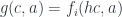
How do we solve this problem? Well, how about creating a global variable to store the audit trail? That’s the simplest solution that comes to mind. And it’s exactly the same method that’s used for standard output in C++, with the global object std::cout. The functions that access a global variable are obviously not pure functions, we are talking about side effects.

string audit;

int logIn(string passwd){
  audit += passwd;
  return 42;
}

double withdraw(int key){
   audit += “withdrawing ”;
   return 100.0;
}

So we have a string, audit, it’s a global variable, and in each of these functions we access this global variable and append something to it. For simplicity, I’m just returning some fake numbers, not to complicate things.

This is not a good solution, for many reasons. It doesn’t scale very well. It’s difficult to maintain. If you want to change the name of the variable, you’d have to go through all this code and modify it. And if, at some point, you decide you want to log more information, not just a string but maybe a timestamp as well, then you have to go through all this code again and modify everything. And I’m not even mentioning concurrency. So this is not the best solution.

But there is another solution that’s really pure. It’s based on the idea that whatever you’re accessing in a function, you should pass explicitly to it, and then return it, with modifications, from the function. That’s pure. So here’s the next solution.

pair<int, string> 
logIn(string passwd, string audit){
  return make_pair(42, audit + passwd);
}

pair<double, string> 
withdraw(int key, string audit){
  return make_pair(100.0
                 , audit + “withdrawing ”);
}

You modify all the functions so that they take an additional argument, the audit string. And the return type is also changed. When we had an int before, it’s now a pair of int and string. When we had a double before, it’s now a pair of double and string. These function now call make_pair before they return, and they put in whatever they were returning before, plus they do this concatenation of a new message at the end of the old audit string. This is a better solution because it uses pure functions. They only depend on their arguments. They don’t have any state, they don’t access any global variables. Every time you call them with the same arguments, they produce the same result.

The problem though is that they don’t memoize that well. Look at the function logIn: you normally get the same key for the same password. But if you want to memoize it when it takes two arguments, you suddenly have to memoize it for all possible histories. Even if you call it with the same password, but the audit string is different, you can’t just access the cache, you have to cache a new pair of values. Your cache explodes with all possible histories.

An even bigger problem is security. Each of these functions has access to the complete log, including the passwords.

Also, each of these functions has to care about things that maybe it shouldn’t be bothered with. It knows about how to concatenate strings. It knows the details of the implementation of the log: that the log is a string. It must know how to accumulate the log.

Now I want to show you a solution that maybe is not that obvious, maybe a little outside of what we would normally think of.

pair<int, string> 
logIn(string passwd){
  return make_pair(42, passwd);
}

pair<double, string> 
withdraw(int key){
  return make_pair(100.0
                  ,“withdrawing ”);
}

We use modified functions, but they don’t take the audit string any more. They just return a pair of whatever they were returning before, plus a string. But each of them only creates a message about what it considers important. It doesn’t have access to any log and it doesn’t know how to work with an audit trail. It’s just doing its local thing. It’s only responsible for its local data. It’s not responsible for concatenation.

It still creates a pair and it has a modified return type.

We have one problem though: we don’t know how to compose these functions. We can’t pass a pair of key and string from logIn to withdraw, because withdraw expects an int. Of course we could extract the int and drop the string, but that would defeat the goal of auditing the code.

Let’s go back a little bit and see how we can abstract this thing. We have functions that used to return some types, and now they return pairs of the original type and a string. This should in principle work with any original type, not just an int or a double. In functional programming we call this “lifting.” Here we lift some type A to a new type, which is a pair of A and a string. Or we can say that we are “embellishing” the return type of a function by pairing it with a string.

I’ll create an alias for this new parameterised type and call it Writer.

template<class A>
using Writer = pair<A, string>;

My functions now return Writers: logIn returns a writer of int, and withdraw returns a writer of double. They return “embellished” types.

Writer<int> logIn(string passwd){
    return make_pair(42, passwd);
}

Writer<double> withdraw(int key){
    return make_pair(100.0, “withdrawing ”);
}

So how do we compose these embellished functions?

In this case we want to compose logIn with withdraw to create a new function called transact. This new function transact will take a password, log the user in, withdraw money, and return the money plus the audit trail. But it will return the audit trail only from those two functions.

Writer<double> transact(string passwd){
  auto p1 logIn(passwd);
  auto p2 withdraw(p1.first);
  return make_pair(p2.first
          , p1.second + p2.second);
}

How is it done? It’s very simple. I call the first function, logIn, with the password. It returns a pair of key and string. Then I call the second function, passing it the first component of the pair — the key. I get a new pair with the money and a string. And then I perform the composition. I take the money, which is the first component of the second pair, and I pair it with the concatenation of the two string that were the second components of the pairs returned by logIn and withdraw.

So the accumulation of the log is done “in between” the calls (think of composition as happening between calls). I have these two functions, and I’m composing them in this funny way that involves the concatenation of strings. The accumulation of the log does not happen inside these two functions, as it happened before. It happens outside. And I can pull out this code and abstract the composition. It doesn’t really matter what functions I’m calling. I can do it for any two functions that return embellished results. I can write generic code that does it and I can call it “compose”.

template<class A, class B, class C>
function<Writer<C>(A)> compose(function<Writer<B>(A)> f
                              ,function<Writer<C>(B)> g)
{
    return [f, g](A x) {
        auto p1 = f(x);
        auto p2 = g(p1.first);
        return make_pair(p2.first
                  , p1.second + p2.second);
    };
}

What does compose do? It takes two functions. The first function takes A and returns a Writer of B. The second function takes a B and return a Writer of C. When I compose them, I get a function that takes an A and returns a Writer of C.

This higher order function just does the composition. It has no idea that there are functions like logIn or withdraw, or any other functions that I may come up with later. It takes two embellished functions and glues them together.

We’re lucky that in modern C++ we can work with higher order functions that take functions as arguments and return other functions.

This is how I would implement the transact function using compose.

Writer<double> transact(string passwd){
  return compose<string, int, double>
           (logIn, withdraw)(passwd);
}

The transact function is nothing but the composition of logIn and withdraw. It doesn’t contain any other logic. I’m using this special composition because I want to create an audit trail. And the audit trail is accumulated “between” the calls — it’s in the glue that glues these two functions together.

This particular implementation of compose requires explicit type annotations, which is kind of ugly. We would like the types to be inferred. And you can do it in C++14 using generalised lambdas with return type deduction. This code was contributed by Eric Niebler.

auto const compose = [](auto f, auto g) {
    return [f, g](auto x) {
        auto p1 = f(x);
        auto p2 = g(p1.first);
        return make_pair(p2.first
                    , p1.second + p2.second);
    };
};

Writer<double> transact(string passwd){
  return compose(logIn, withdraw)(passwd);
}

Back to Categories

Now that we’ve done this example, let’s go back to where we started. In category theory we have functions and we have composition of functions. Here we also have functions and composition, but it’s a funny composition. We have functions that take simple types, but they return embellished types. The types don’t match.

Let me remind you what we had before. We had a category of types and pure functions with the obvious composition.

• Objects: types,
• Arrows: pure functions,
• Composition: pass the result of one function as the argument to another.

What we have created just now is a different category. Slightly different. It’s a category of embellished functions. Objects are still types: Types A, B, C, like integers, doubles, strings, etc. But an arrow from A to B is not a function from type A to type B. It’s a function from type A to the embellishment of the type B. The embellished type depends on the type B — in our case it was a pair type that combined B and a string — the Writer of B.

Now we have to say how to compose these arrows. It’s not as trivial as it was before. We have one arrow that takes A into a pair of B and string, and we have another arrow that takes B into a pair of C and string, and the composition should take an A and return a pair of C and string. And I have just defined this composition. I wrote code that does this:

auto const compose = [](auto f, auto g) {
    return [f, g](auto x) {
        auto p1 = f(x);
        auto p2 = g(p1.first);
        return make_pair(p2.first
                    , p1.second + p2.second);
    };
};

So do we have a category here? A category that’s different from the original category? Yes, we do! It has composition and it has identity.

What’s its identity? It has to be an arrow from the object to itself, from A to A. But an arrow from A to A is a function from A to a pair of A and string — to a Writer of A. Can we implement something like this? Yes, easily. We will return a pair that contains the original value and the empty string. The empty string will not contribute to our audit trail.

template<class A>
Writer<A> identity(A x) {
    return make_pair(x, "");
}

Is this composition associative? Yes, it is, because the underlying composition is associative, and the concatenation of strings is associative.

We have a new category. We have incorporated side effects by modifying the original category. We are still only using pure functions and yet we are able to accumulate an audit trail as a side effect. And we moved the side effects to the definition of composition.

It’s a funny new way of looking at programming. We usually see the functions, and the data being passed between functions, and here suddenly we see a new dimension to programming that is orthogonal to this, and we can manipulate it. We change the way we compose functions. We have this new power to change composition. We have a new way of solving problems by moving to these embellished functions and defining a new way of composing them. We can define new combinators to compose functions, and we’ll let the combinators do some work that we don’t want these functions to do. We can factor these things out and make them orthogonal.

Does this approach generalize?

One easy generalisation is to observe that the Writer structure works for any monoid. It doesn’t have to be just strings. Look at how composition and identity are defined in our new cateogory. The only properties of the log we are using are concatenation and unit. Concatenation must be associative for the composition to be associative. And we need a unit of concatenation so that we can define identity in our category. We don’t need anything else. This construction will work with any monoid.

And that’s great because you have one more dimension in which you can modify your code without touching the rest. You can change the format of the log, and all you need to modify in your code is compose and identity. You don’t have to go through all your functions and modify the code. They will still work because all the concatenation of logs is done inside compose.

Kleisli Categories

This was just a little taste of what is possible with category theory. The thing I called embellishment is called a functor in category theory. You can implement categorical functors in C++. There are all kinds of embellishments/functors that you can use here. And now I can tell you the secret: this funny composition of functions with the funny identity is really a monad in disguise. A monad is just a funny way of composing embellished functions so that they form a category. A category based on a monad is called a Kleisli category.

Are there any other interesting monads that I can use this construction with? Yes, lots! I’ll give you one example. Functions that return futures. That’s our new embellishment. Give me any type A and I will embellish it by making it into a future. This embellishment also produces a Kleisli category. The composition of functions that return futures is done through the combinator “then”. You call one function returning a future and compose it with another function returning a future by passing it to “then.” You can compose these function into chains without ever having to block for a thread to finish. And there is an identity, which is a function that returns a trivial future that’s always ready. It’s called make_ready_future. It’s an arrow that takes A and returns a future of A.

Now you understand what’s really happening. We are creating this new category based on future being a monad. We have new words to describe what we are doing. We are reusing an idea from category theory to solve a completely different problem.

Resumable Functions

There is one little invonvenience with this approach. It requires writing a lot of so called “boilerplate” code. Repetitive code that obscures the simple logic. Here it’s the glue code, the “compose” and the “then.” What you’d like to do is to write your code directly in terms of embellished function, and the composition to be implicit. People noticed this and came up with solutions. In case of futures, the practical solution is called resumable functions.

Resumable functions are designed to hide the composition of functions that return futures. Here’s an example.

int cnt = 0;
do
{
   cnt = await streamR.read(512, buf);
   if ( cnt == 0 ) break;
   cnt = await streamW.write(cnt, buf);
} while (cnt > 0);

This code copies a file using a buffer, but it does it asynchronously. We call a function read that’s asynchronous. It doesn’t immediately fill the buffer, it returns a future instead. Then we call the function write that’s also asynchronous. We do it in a loop.

This code looks almost like sequential code, except that it has these await keywords. These are the points of insertion of our composition. These are the places where the code is chopped into pieces and composed using then.

I won’t go into details of the implementation. The point is that the composition of these embellished functions is almost entirely hidden. It doesn’t look like composition in a Kleisli category, but it really is.

This solution is usually described at a very low level, in terms of coroutines implemented as state machines with static variables and gotos. And what is being lost in all this engineering talk is how general this idea is — the idea of overloading composition to build a category of embellished functions.

Just to drive this home, here’s an example of different code that does completely different stuff. It calculates Fibonacci numbers on demand. It’s a generator of Fibonacci numbers.

generator<int> fib() 
{
    int a = 0; 
    int b = 1; 
    for (;;) { 
        __yield_value a; 
        auto next = a + b; 
        a = b; 
        b = next; 
    } 
}

Instead of await it has __yield_value. But it’s the same idea of resumable functions, only with a different monad. This monad is called a list monad. And this kind of code in combination with Eric Niebler’s proposed range library could lead to very powerful programming idioms.

Conclusion

Why do we have to separate the two notions: that of resumable functions and that of generators, if they are based on the same abstraction? Why do we have to reinvent the wheel?

There’s this great opportunity for C++, and I’m afraid it will be missed like so many other opportunities for great generalisations that were missed in the past. It’s the opportunity to introduce one general solution based on monads, rather than keep creating ad-hoc solutions, one problem at a time. The same very general pattern can be used to control all kinds of side effects. It can be used for auditing, exceptions, ranges, futures, I/O, continuations, and all kinds of user-defined monads.

This amazing power could be ours if we start thinking in more abstract terms, if we reach into category theory.

The main idea of functional programming is to treat functions like any other data types. In particular, we want to be able to pass functions as arguments to other functions, return them as values, and store them in data structures. But what kind of data type is a function? It’s a type that, when paired with another piece of data called the argument, can be passed to a function called apply to produce the result.

apply :: (a -> d, a) -> d

In practice, function application is implicit in the syntax of the language. But, as we will see, even if your language doesn’t support higher-order functions, all you need is to roll out your own apply.

But where do these function objects, arguments to apply, come from; and how does the built-in apply know what to do with them?

When you’re implementing a function, you are, in a sense, telling apply what to do with it–what code to execute. You’re implementing individual chunks of apply. These chunks are usually scattered all over your program, sometimes anonymously in the form of lambdas.

We’ll talk about program transformations that introduce more functions, replace anonymous functions with named ones, or turn some functions into data types, without changing program semantics. The main advantage of such transformations is that they may improve performance, sometimes drastically so; or support distributed computing.

Function Objects

As usual, we look to category theory to provide theoretical foundation for defining function objects. It turns out that we are able to do functional programming because the category of types and functions is cartesian closed. The first part, cartesian, means that we can define product types. In Haskell, we have the pair type (a, b) built into the language. Categorically, we would write it as . Product is functorial in both arguments so, in particular, we can define a functor

   

It’s really a family of functors that it parameterized by .

The right adjoint to this functor

   

defines the function type (a.k.a., the exponential object ). The existence of this adjunction is what makes a category closed. You may recognize these two functors as, respectively, the writer and the reader functor. When the parameter is restricted to monoids, the writer functor becomes a monad (the reader is already a monad).

An adjunction is defined as a (natural) isomorphism of hom-sets:

   

or, in our case of two endofunctors, for some fixed ,

   

In Haskell, this is just the definition of currying:

curry   :: ((c, a) -> d)   -> (c -> (a -> d))
uncurry :: (c -> (a -> d)) -> ((c, a) -> d)

You may recognize the counit of this adjunction

   

as our apply function

   

Adjoint Functor Theorem

In my previous blog post I discussed the Freyd’s Adjoint Functor theorem from the categorical perspective. Here, I’m going to try to give it a programming interpretation. Also, the original theorem was formulated in terms of finding the left adjoint to a given functor. Here, we are interested in finding the right adjoint to the product functor. This is not a problem, since every construction in category theory can be dualized by reversing the arrows. So instead of considering the comma category , we’ll work with the comma category . Its objects are pairs , in which is a morphism

    .

This is the general picture but, in our case, we are dealing with a single category, and is an endofunctor. We can implement the objects of our comma category in Haskell

data Comma a d c = Comma c ((c, a) -> d)

The type a is just a parameter, it parameterizes the (left) functor

   

and d is the target object of the comma category.

We are trying to construct a function object representing functions a->d, so what role does c play in all of this? To understand that, you have to take into account that a function object can be used to describe closures: functions that capture values from their environment. The type c represents those captured values. We’ll see this more explicitly later, when we talk about defunctionalizing closures.

Our comma category is a category of all closures that go from to while capturing all possible environments. The function object we are constructing is essentially a sum of all these closures, except that some of them are counted multiple times, so we need to perform some identifications. That’s what morphisms are for.

The morphisms of the comma category are morphisms in that make the following triangles in commute.

Unfortunately, commuting diagrams cannot be expressed in Haskell. The closest we can get is to say that a morphism from

c1 :: Comma a d c

to

c2 :: Comma a d c'

is a function h :: c -> c' such that, if

c1 = Comma c f
f :: (c, a) -> d
c2 = Comma c' g
g :: (c', a) -> d

then

f = g . bimap h id

Here, bimap h id is the lifting of h to the functor . More explicitly

f (c, x) = g (h c, x)

As we are interpreting c as the environment in which the closure is defined, the question is: does f use all of the information encoded in c or just a part of it? If it’s just a part, then we can factor it out. For instance, consider a lambda that captures an integer, but it’s only interested in whether the integer is even or odd. We can replace this lambda with one that captures a Boolean, and use the function even to transform the environment.

The next step in the construction is to define the projection functor from the comma category back to that forgets the part and just keeps the object

   

We use this functor to define a diagram in . Now, instead of taking its limit, as we did in the previous installment, we’ll take the colimit of this diagram. We’ll use this colimit to define the action of the right adjoint functor on .

   

In our case, the forgetful functor discards the function part of Comma a d c, keeping only the environment . This means that, as long as d is not Void, we are dealing with a gigantic diagram that encompasses all objects in our category of types. The colimit of this diagram is a gigantic coproduct of everything, modulo identifications introduced by morphisms of the comma category. But these identifications are crucial in pruning out redundant closures. Every lambda that uses only part of the information from the captured environment can be identified with a simpler lambda that uses a simplified environment.

For illustration, consider a somewhat extreme case of constructing the function object , or ( to the power of the terminal object). This object should be isomorphic to . Let’s see how this works: The terminal object is the unit of the product, so

   

so the comma category is just the slice category of arrows to . It so happens that this category has the terminal object . The colimit of a diagram that has a terminal object is that terminal object. So, indeed, in this case, our construction produces a function object that is isomorphic to .

   

Intuitively, given a lambda that captures a value of type from the environment and returns a , we can trivially factor it out, using this lambda to transform the environment for to and then apply the identity on . The latter corresponds to the comma category object , and the forgetful functor maps it to .

It’s instructive to run a few more examples to get the hang of it. For instance, the function object Bool->d can be constructed by considering closures of the type

f :: (c, Bool) -> d

Any such closure can be factorized by the following transformation of the environment

h :: c -> (d, d)
h c = (f (c, True), f (c, False))

followed by

g :: ((d, d), Bool) -> d
g ((d1, d2), b) = if b then d1 else d2

Indeed:

f (c, b) = g (h c, b)

In other words
   
where corresponds to the Bool type.

Counit

We are particularly interested in the counit of the adjunction. Its component at is a morphism

   

It also happens to be an object in the comma category, namely

    .

In fact, it is the terminal object in that category. You can see that because for any other object there is a morphism that makes the following triangle commute:

This morphisms is a leg in the terminal cocone that defines . We know for sure that is in the base of that cocone, because it’s the projection of .

To get some insight into the construction of the function object, imagine that you can enumerate the set of all possible environments . The comma category would then consist of pairs . The coproduct of all those environments is a good candidate for the function object . Indeed, let’s try to define a counit for it:

   

I used the distributive law:

   

and the fact that the mapping out of a sum is the product of mappings. The right hand side can be constructed from the morphisms of the comma category.

So the object satisfies at least one requirement of the function object: there is an implementation of apply for it. It is highly redundant, though. This is why, instead of the coproduct, we used the colimit in our construction of the function object. Also, we ignored the size issues.

Size Issues

As we discussed before, this construction doesn’t work in general because of size issues: the comma category is not necessarily small, and the colimit might not exist.

To address this problems, we have previously defined small solution sets. In the case of the right adjoint, a solution set is a family of objects that is weakly terminal in . These are pairs that, among themselves, can factor out any

   

It means that we can always find an index and a morphism to satisfy that equation. Every might require a different and to factor through but, for any , we are guaranteed to always find a pair.

Once we have a complete solution set, the right adjoint is constructed by first forming a coproduct of all the and then using a coequalizer to construct one terminal object.

What is really interesting is that, in some cases, we can just use the coproduct of the solution set, to approximate the adjoint (thus skipping the equalizer part).

The idea is that, in a particular program, we don’t need to represent all possible function types, just a (small) subset of those. We are also not particularly worried about uniqueness: it’s no problem if the same function ends up with multiple syntactic representations.

Let’s reformulate Freyd’s construction of the function object in programming terms. The solution set is the set of types and functions

such that, for any function

that is of interest in our program (for instance, used as an argument to another function) there exists an and a function

such that can be rewritten as

In other words, every function of interest can be replaced by one of the solution-set functions. The environment for this standard function can be always extracted from the environment of the more general function.

CPS Transformation

A particular application of higher order functions shows up in the context of continuation passing transformation. Let’s look at a simple example. We are going to implement a function that traverses a binary tree containing strings, and concatenates them all into one string. Here’s the tree

data Tree = Leaf String 
          | Node Tree String Tree

Recursive traversal is pretty straightforward

show1 :: Tree -> String
show1 (Leaf s) = s
show1 (Node l s r) =
  show1 l ++  s ++ show1 r

We can test it on a small tree:

tree :: Tree
tree = Node (Node (Leaf "1 ") "2 " (Leaf "3 "))
            "4 " 
            (Leaf "5 ")

test = show1 tree

There is just one problem: recursion consumes the runtime stack, which is usually a limited resource. Your program may run out of stack space resulting in the “stack overflow” runtime error. This is why the compiler will turn recursion into iteration, whenever possible. And it is always possible if the function is tail recursive, that is, the recursive call is the last call in the function. No operation on the result of the recursive call is permitted in a tail recursive function.

This is clearly not happening in our implementation of show1: After the recursive call is made to traverse the left subtree, we still have to make another call to traverse the right tree, and the two results must be concatenated with the contents of the node.

Notice that this is not just a functional programming problem. In an imperative language, where iteration is the rule, tree traversal is still implemented using recursion. That’s because the data structure itself is recursive. It used to be a common interview question to implement non-recursive tree traversal, but the solution is always to explicitly implement your own stack (we’ll see how it’s done at the end of this post).

There is a standard procedure to make functions tail recursive using continuation passing style (CPS). The idea is simple: if there is stuff to do with the result of a function call, let the function we’re calling do it instead. This “stuff to do” is called a continuation. The function we are calling takes the continuation as an argument and, when it finishes its job, it calls it with the result. A continuation is a function, so CPS-transformed functions have to be higher-order: they must accept functions as arguments. Often, the continuations are defined on the spot using lambdas.

Here’s the CPS transformed tree traversal. Instead of returning a string, it accepts a continuation k, a function that takes a string and produces the final result of type a.

show2 :: Tree -> (String -> a) -> a
show2 (Leaf s) k = k s
show2 (Node lft s rgt) k =
  show2 lft (\ls -> 
    show2 rgt (\rs -> 
      k (ls ++ s ++ rs)))

If the tree is just a leaf, show2 calls the continuation with the string that’s stored in the leaf.

If the tree is a node, show2 calls itself recursively to convert the left child lft. This is a tail call, nothing more is done with its result. Instead, the rest of the work is packaged into a lambda and passed as a continuation to show2. This is the lambda

\ls -> 
    show2 rgt (\rs -> 
      k (ls ++ s ++ rs))

This lambda will be called with the result of traversing the left child. It will then call show2 with the right child and another lambda

\rs -> 
      k (ls ++ s ++ rs)

Again, this is a tail call. This lambda expects the string that is the result of traversing the right child. It concatenates the left string, the string from the current node, and the right string, and calls the original continuation k with it.

Finally, to convert the whole tree t, we call show2 with a trivial continuation that accepts the final result and immediately returns it.

show t = show2 t (\x -> x)

There is nothing special about lambdas as continuations. It’s possible to replace them with named functions. The difference is that a lambda can implicitly capture values from its environment. A named function must capture them explicitly. The three lambdas we used in our CPS-transformed traversal can be replaced with three named functions, each taking an additional argument representing the values captured from the environment:

done s = s
next (s, rgt, k) ls = show3 rgt (conc (ls, s, k))
conc (ls, s, k) rs = k (ls ++ s ++ rs)

The first function done is an identity function, it forces the generic type a to be narrowed down to String.

Here’s the modified traversal using named functions and explicit captures.

show3 :: Tree -> (String -> a) -> a
show3 (Leaf s) k = k s
show3 (Node lft s rgt) k =
  show3 lft (next (s, rgt, k))

show t = show3 t done

We can now start making the connection with the earlier discussion of the adjoint theorem. The three functions we have just defined, done, next, and conc, form the family

    .

They are functions of two arguments, or a pair of arguments. The first argument represents the object , part of the solution set. It corresponds to the environment captured by the closure. The three are, respectively

()
(String, Tree, String -> String)
(String, String, String->String)

(Notice the empty environment of done, here represented as the unit type ().)

The second argument of all three functions is of the type String, and the return type is also String so, according to Freyd’s theorem, we are in the process of defining the function object , where is String and is String.

Defunctionalization

Here’s the interesting part: instead of defining the general function type String->String, we can approximate it with the coproduct of the elements of the solution set. Here, the three components of the sum type correspond to the environments captured by our three functions.

data Kont = Done 
          | Next String Tree   Kont 
          | Conc String String Kont

The counit of the adjunction is approximated by a function from this sum type paired with a String, returning a String

apply :: Kont -> String -> String
apply Done s = s
apply (Next s rgt k) ls = show4 rgt (Conc ls s k)
apply (Conc ls s k) rs  = apply k (ls ++ s ++ rs)

Rather than passing one of the three functions to our higher-order CPS traversal, we can pass this sum type

show4 :: Tree -> Kont -> String
show4 (Leaf s) k = apply k s
show4 (Node lft s rgt) k = 
  show4 lft (Next s rgt k)

This is how we execute it

show t = show4 t Done

We have gotten rid of all higher-order functions by replacing their function arguments with a data type equipped with the apply function. There are several situations when this is advantageous. In procedural languages, defunctionalization may be used to replace recursion with loops. In fact, the Kont data structure can be seen as a user-defined stack, especially if it’s rewritten as a list.

type Kont = [(String, Either Tree String)]

Here, Done was replaced with an empty list and Next and Conc together correspond to pushing a value on the stack.

In Haskell, the compiler performs tail recursion optimization, but defunctionalization may still be useful in implementing distributed systems, or web servers. Any time we need to pass a function between a client and a server, we can replace it by a data type that can be easily serialized.

Bibliography

1. John C. Reynolds, Definitional Interpreters for Higher-Order Programming Languages
2. James Koppel, The Best Refactoring You’ve Never Heard Of.