In my last blog post I talked about a universal construction of a product in an arbitrary category. This kind of construction might seem very abstract to you and me, but not to a mathematician. Every step in that construction may be analyzed under a microscope and further generalized.

Let’s start with the selection of two objects whose product we are defining. What does it mean to select two objects in a category C? In any other branch of mathematics that would be a stupid question, but not in category theory. You select two objects by providing a functor from a two-object category to C.

You might be used to thinking of categories as those big hulking things, like the category of sets or monoids. But there are also dwarf categories that consist of one or two objects and just a handful of arrows between them. They don’t represent anything other than simple graphs. In particular, the simplest non-trivial category, called 1, is just a single object with one identity morphism looping back on itself. We can define a functor from that category to any other category. It will map the single object to a particular object in the target category. (It will also map the only morphism into the identity morphism for that target object.) This functor is the essence of picking an object in a category. Instead of saying “Pick an object in the category C,” you may say “Give me a functor from the singleton category to C.”

The next simplest category is a two-object category, {1, 2}. We have two objects and two identity morphisms acting on them. Assume there are no morphisms between the two objects (so it’s a “discrete” category). A functor F from this category to C is the essence of picking two objects in C.

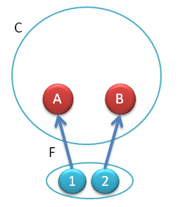
Fig 1. Functor F from {1,2} to C

Actually, there is an even simpler functor from {1, 2} to C, a degenerate functor that picks just one object in C — it maps both object to the same object in C. We’ll call this functor Δ_X, where X is the target object in C.

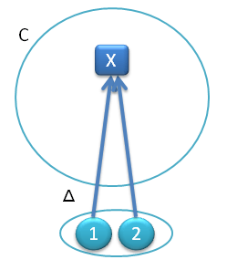
Fig 2. Const functor from {1, 2} to C

When there are two functors, there may be a natural transformation between them. Let’s try to define such a transformation between Δ_X and F. The first functor, Δ_X, maps both objects 1 and 2 to X. The second, F, maps 1 to A and 2 to B. A natural transformation between these two functors has two components: the first is a morphism p1 from X to A, and the second is a morphism p2 from X to B.

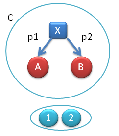
Fig 3. Components of the natural transformation from the constant functor Δ to F

But that’s exactly one of the triples (X, p1, p2) that I used in the definition of a product in my previous post. The product was defined as the universal triple with a unique mapping from any other triple to it.

We no longer have to talk about selecting objects and constructing triples. Instead we can talk about natural transformations between the constant functor and a functor from the category {1, 2} to C.

This might not sound like a great simplification, but it’s an essential step toward the next generalization. We are going to replace the simple category {1, 2} with an arbitrary category J (sometimes called an index category). Again, we have the constant functor Δ_X from J to C, which maps all objects in J to a single object X. It also maps all morphisms in J to a single identity morphism i_X. We also have the functor F that embeds J in C, but it will now map morphisms as well as objects. It’s helpful to think of J as a graph with vertices and arrows. F embeds this graph into C. As before, a natural transformation from Δ_X to F has as its components morphisms going from X to the vertices of the diagram defined by F. Because of its conical shape, this natural transformation is called a cone.

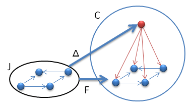
Fig 5. A cone

But a natural transformation not only acts between objects but also between morphisms. In fact “naturality” is defined in terms of morphisms.

Fig 6 illustrates the general case. We have two functors F and G. These functors map objects X and Y, respectively, to FX, FY, and GX, GY.

A morphism f from X to Y is mapped by F to Ff and by G to Gf.

On top of that, we have the natural transformation Φ from F to G, whose components are Φ_X and Φ_Y. For Φ to be natural these four arrows must form a commutative diagram. In other words:

Gf . ΦX = ΦY . Ff

Fig 6. Naturality square

Replace F with Δ_X and you’ll see that the naturality condition for our cone translates into the commutativity of all the triangles with the vertex X. We didn’t see this condition in the product example, because there the base of the cone had no arrows. So let’s find a better example.

Equilizer

A lot of practical math problems boil down to solving an equation or two. An equation usually has the form: A function of some variable is equal to zero. The set of solutions is called a kernel. But this definition assumes that there is a zero, and that’s too specific. A more general formulation talks about two functions being equal. A set of values on which two functions are equal is called the equilizer. So the equilizer is the generalization of the kernel of the difference of two functions. It will work even if we don’t know what zero is or how to subtract values.

Let’s dissect this definition further. We have two functions, f and g, from A to B. The equilizer is the subset of A on which f and g are equal. How can we generalize this definition so that we don’t have to think about elements of A and B? We have two problems: how to define a subset and how to define the equality of elements.

Let’s start with the subset. We can look at a subset as an embedding of one set inside another. Every function, in a matter of speaking, defines an embedding of its domain into its co-domain. For instance, a function from real numbers to 3-d points can be viewed as an embedding of a line in space.

Let’s see how far we can get with this idea for the purpose of defining the equilizer of f and g. We need another set X and a function p from X to A. The image of X in A will serve as our definition of a subset of A. Now let’s apply the function f after p. We get a composite function f . p from X to B. Similarly, we can apply g after p to get g . p. In general, these two composite functions will be different, except when the image of p falls inside the equilizer of f and g. Notice that we can talk about equality of functions without resorting to equality of elements if we look at them as morphisms in a category.

You see where this is heading? The set X with a function p, while not exactly defining the equilizer, provides some sort of a candidate for it. This candidate can be fully described in categorical terms as an object and a morphism, without recourse to sets or their elements. And the equality

f . p = g . p

is just the condition for the following diagram to commute:

Fig 7. The equilizer cone

But this is a cone for a two-object-two-arrow category! The objects A and B and the morphisms f and g can be seen as the image of this category under some functor F. Likewise, the object X is the image of this category under the constant functor Δ_X. The two orange arrows are the components of the natural transformation from Δ_X to F, and the commutativity of this diagram is nothing but its naturality condition.

Of course, there may be many pairs (X, p) that satisfy our conditions. We are looking for the universal one, with the property that any other pair (Y, q) can be mapped into it.

Fig 8. X is the equilizer if its cone is universal

Just like in the product case, we have to demand that q factorizes through h, or that the appropriate triangles commute — in particular q = p . h. This universal cone is the equilizer.

The Moment of Zen

You might ask yourself the question: Why should I care whether some diagrams commute or not? In particular, why are natural transformations better than the “unnatural” ones? Why is it important that naturality diagrams commute? There must be something incredibly deep behind this idea of commutativity to make it pop up in so many diverse branches of mathematics unified by category theory.

Indeed, the very definition of category contains the mother of all commuting diagrams: The condition that, if there is a morphism from A to B and another from B to C, then there is a shortcut morphism from A to C, and it doesn’t matter which way you go. This is the essence of composability: you decompose the path from A to C into its components.

Every programmer is familiar with the idea of functional decomposition, but this pattern goes much deeper than just programming. It’s the essence of our knowledge, of our understanding. We don’t understand anything unless we are able to split it into smaller steps and then put these steps back together — compose them. Without composition we can’t deal with complexity.

The other foundation of understanding is the ability to create models. We create simple models of complex phenomena all the time. By understanding how models work, we gain insight into how complex phenomena work. But for that we need to establish the correspondence, the mapping, between the domain of the model and the domain of the phenomenon that we’re studying. And what’s the most important property of that mapping? Well, our understanding of the model is built on our understanding of its parts and of the ways they compose. So the mapping must preserve composability! Mappings that preserve composability are called functors.

We’ve used some very simple categories as our models. The {1, 2} category modeled the selection of two objects. We used a functor to embed this model into a bigger category C. In that particular case, there wasn’t much structure for the functor to preserve. The model for the equilizer, on the other hand, was a bit more involved. Besides the two objects, it also had two parallel arrows. The functor that embedded this model had to map those arrows as well.

If functors are used for modeling, what are natural transformations? They relate different phenomena described by the same model.

A stick figure is a model for a human being. It can be mapped into Alice, or it can be mapped into Bob. A natural transformation would map Alice into Bob in such a way as to preserve the stick-figure structure. So if the circle is mapped into Alice’s head by one functor, and into Bob’s head by another, a natural transformation would map Alice’s head into Bob’s head.

The model tells us that there is a neck between the head and the torso. So we could use Alice’s neck to go from her head to her torso, and then map her torso to Bob’s torso using the natural transformation. But we could also map Alice’s head to Bob’s head using the natural transformation, and then use Bob’s neck to get to his torso. Naturality tells us that it doesn’t matter which way we go, the result is the same.

We also have the constant functor, which maps the model into a single blob. A natural transformation then maps this blob into Bob; again, with the condition that it doesn’t matter whether we reach Bob’s torso from the blob through his right hand and arm or through his left hand and arm.

Now take into account that, although the stick figure is just made of points and lines, it is mapped into real human beings and real blobs. So a morphism from a blob to Bob’s hand is not trivial, and there may be many different ones. Similarly, the arm that connects the hand to the torso contains veins, arteries, nerves, etc. So naturality is a non-trivial condition, especially if the blob itself is complex.

So what is special about the universal blob? It has to have some interesting internal structure because it not only maps into every part of Bob, but it maps better than any other blob. Any other blob that maps naturally into Bob also maps into the universal blob. And it maps in such a way that it doesn’t matter if you go directly from the said blob to Bob, or if you go through the universal blob. The universal blob contains the stick-figure essence of Bob, and no other blob (that is not isomorphic to it) can take its place.

Universality tells us something about the structure of an object not by dissecting it but by describing its relationship to other objects that model a certain relationship.

Limits

Having defined a cone as a natural transformation from Δ_X to F — two functors that map the category J to category C — we can now define the limit of F as the universal cone. For that, we need a way to compare cones that differ only by their top vertex. If there is a universal cone with the top vertex U, then any other cone with the top vertex V can be uniquely mapped onto it. It must be a mapping that preserves the structure of the cone, so if h maps V into U, h must factorize all the arrows that form the V cone into the arrows that form the U cone. For instance, in Fig 9, we must have q = p . h, etc.

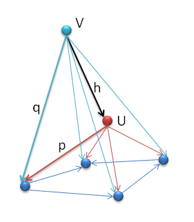
Fig 9. The limit U is the vertex of the universal cone

But there’s a better way of looking at it. Notice that, in the definition of a limit, we establish a one to one correspondence between a cone with the vertex V and a morphism h from V to U. The definition talks about there being a unique h for every cone, but the other way around works as well. Given an h we can construct the cone at V by composing the morphisms — as in q = p . h.

A cone is a natural transformation, a member of Nat(Δ_V, F), the set of natural transformation between two functors, Δ_V and F. A morphism h is a member of the home set Hom(V, U), the set of morphisms between two objects. So we can say that if U is a limit of F then there is an isomorphism between those two sets:

Nat(ΔV, F) ~ Hom(V, U)

In fact, if we insist that this isomorphism be natural, we’ll get all the commuting triangles for free. Remember? Naturality condition is just the commutability of certain diagrams. So if there is a natural isomorphism between these two sets, then U is a limit of F. In fact, we can use this isomorphism as the definition of the limit.

But what does it mean that the isomorphism is natural? What are the two functors that are mapped by it? One functor maps V into Hom(V, U), and the other maps V into Nat(Δ_V, F). Both Hom(V, U) and Nat(Δ_V, F) are sets in the category of sets. So these are functors from C to Set. You might recognize the first one from the Yoneda lemma.

The second one is a bit more tricky. To understand it, you have to realize that functors themselves form a category. If functors are object in the functor category than natural transformations between these functors are morphisms. Natural transformations compose (and their composition is associative), and there always is a unit natural transformation for each functor. So this is a legitimate category. A hom set in that category is a set of all natural transformations between two functors. Nat(Δ_V, F) is one such hom set.

Whenever you see a natural isomorphism of hom sets, chances are there is an adjunction between two functors. A functor F is said to be left adjoint to the functor G (or G right adjoint to F) if the following two hom sets are naturally isomorphic:

Hom(FX, Y) ~ Hom(X, GY)

If you compare this with our definition of a limit, you’ll see that the functor that maps F to its limit U is right adjoint to the const functor Δ_V. Of course this is only true if the said functor exists, which is not always true — not all diagrams of shape J must have limits in C.

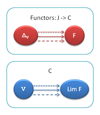
The adjunction between Δ_V and Lim F (limit of F) is the natural isomorphism between the corresponding hom sets (arrows).

I hope to talk more about adjoint functors in the future.

Videography

Hopefully this blog post will prepare you to watch this excellent series of videos by Catsters on YouTube:

1. Cones and limits: Definitions.
2. Examples of limits: Terminal object, product, pullback, equalizer.
3. Cones as natural transformations.
4. Formal definition of limit as natural isomorphism.
5. Limits and adjunctions.
6. Colimits.