Category Theory


Categories for Programmers. Previously Products and Coproducts. See the Table of Contents.

We’ve seen two basic ways of combining types: using a product and a coproduct. It turns out that a lot of data structures in everyday programming can be built using just these two mechanisms. This fact has important practical consequences. Many properties of data structures are composable. For instance, if you know how to compare values of basic types for equality, and you know how to generalize these comparisons to product and coproduct types, you can automate the derivation of equality operators for composite types. In Haskell you can automatically derive equality, comparison, conversion to and from string, and more, for a large subset of composite types.

Let’s have a closer look at product and sum types as they appear in programming.

Product Types

The canonical implementation of a product of two types in a programming language is a pair. In Haskell, a pair is a primitive type constructor; in C++ it’s a relatively complex template defined in the Standard Library.

Pair

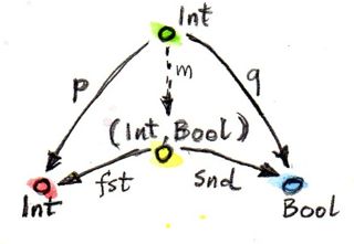
Pairs are not strictly commutative: a pair (Int, Bool) cannot be substituted for a pair (Bool, Int), even though they carry the same information. They are, however, commutative up to isomorphism — the isomorphism being given by the swap function (which is its own inverse):

swap :: (a, b) -> (b, a)
swap (x, y) = (y, x)

You can think of the two pairs as simply using a different format for storing the same data. It’s just like big endian vs. little endian.

You can combine an arbitrary number of types into a product by nesting pairs inside pairs, but there is an easier way: nested pairs are equivalent to tuples. It’s the consequence of the fact that different ways of nesting pairs are isomorphic. If you want to combine three types in a product, a, b, and c, in this order, you can do it in two ways:

((a, b), c)

or

(a, (b, c))

These types are different — you can’t pass one to a function that expects the other — but their elements are in one-to-one correspondence. There is a function that maps one to another:

alpha :: ((a, b), c) -> (a, (b, c))
alpha ((x, y), z) = (x, (y, z))

and this function is invertible:

alpha_inv :: (a, (b, c)) -> ((a, b), c)
alpha_inv  (x, (y, z)) = ((x, y), z)

so it’s an isomorphism. These are just different ways of repackaging the same data.

You can interpret the creation of a product type as a binary operation on types. From that perspective, the above isomorphism looks very much like the associativity law we’ve seen in monoids:

(a * b) * c = a * (b * c)

Except that, in the monoid case, the two ways of composing products were equal, whereas here they are only equal “up to isomorphism.”

If we can live with isomorphisms, and don’t insist on strict equality, we can go even further and show that the unit type, (), is the unit of the product the same way 1 is the unit of multiplication. Indeed, the pairing of a value of some type a with a unit doesn’t add any information. The type:

(a, ())

is isomorphic to a. Here’s the isomorphism:

rho :: (a, ()) -> a
rho (x, ()) = x
rho_inv :: a -> (a, ())
rho_inv x = (x, ())

These observations can be formalized by saying that Set (the category of sets) is a monoidal category. It’s a category that’s also a monoid, in the sense that you can multiply objects (here, take their cartesian product). I’ll talk more about monoidal categories, and give the full definition in the future.

There is a more general way of defining product types in Haskell — especially, as we’ll see soon, when they are combined with sum types. It uses named constructors with multiple arguments. A pair, for instance, can be defined alternatively as:

data Pair a b = P a b

Here, Pair a b is the name of the type paremeterized by two other types, a and b; and P is the name of the data constructor. You define a pair type by passing two types to the Pair type constructor. You construct a pair value by passing two values of appropriate types to the constructor P. For instance, let’s define a value stmt as a pair of String and Bool:

stmt :: Pair String Bool
stmt = P "This statements is" False

The first line is the type declaration. It uses the type constructor Pair, with String and Bool replacing a and the b in the generic definition of Pair. The second line defines the actual value by passing a concrete string and a concrete Boolean to the data constructor P. Type constructors are used to construct types; data constructors, to construct values.

Since the name spaces for type and data constructors are separate in Haskell, you will often see the same name used for both, as in:

data Pair a b = Pair a b

And if you squint hard enough, you may even view the built-in pair type as a variation on this kind of declaration, where the name Pair is replaced with the binary operator (,). In fact you can use (,) just like any other named constructor and create pairs using prefix notation:

stmt = (,) "This statement is" False

Similarly, you can use (,,) to create triples, and so on.

Instead of using generic pairs or tuples, you can also define specific named product types, as in:

data Stmt = Stmt String Bool

which is just a product of String and Bool, but it’s given its own name and constructor. The advantage of this style of declaration is that you may define many types that have the same content but different meaning and functionality, and which cannot be substituted for each other.

Programming with tuples and multi-argument constructors can get messy and error prone — keeping track of which component represents what. It’s often preferable to give names to components. A product type with named fields is called a record in Haskell, and a struct in C.

Records

Let’s have a look at a simple example. We want to describe chemical elements by combining two strings, name and symbol; and an integer, the atomic number; into one data structure. We can use a tuple (String, String, Int) and remember which component represents what. We would extract components by pattern matching, as in this function that checks if the symbol of the element is the prefix of its name (as in He being the prefix of Helium):

startsWithSymbol :: (String, String, Int) -> Bool
startsWithSymbol (name, symbol, _) = isPrefixOf symbol name

This code is error prone, and is hard to read and maintain. It’s much better to define a record:

data Element = Element { name         :: String
                       , symbol       :: String
                       , atomicNumber :: Int }

The two representations are isomorphic, as witnessed by these two conversion functions, which are the inverse of each other:

tupleToElem :: (String, String, Int) -> Element
tupleToElem (n, s, a) = Element { name = n
                                , symbol = s
                                , atomicNumber = a }
elemToTuple :: Element -> (String, String, Int)
elemToTuple e = (name e, symbol e, atomicNumber e)

Notice that the names of record fields also serve as functions to access these fields. For instance, atomicNumber e retrieves the atomicNumber field from e. We use atomicNumber as a function of the type:

atomicNumber :: Element -> Int

With the record syntax for Element, our function startsWithSymbol becomes more readable:

startsWithSymbol :: Element -> Bool
startsWithSymbol e = isPrefixOf (symbol e) (name e)

We could even use the Haskell trick of turning the function isPrefixOf into an infix operator by surrounding it with backquotes, and make it read almost like a sentence:

startsWithSymbol e = symbol e `isPrefixOf` name e

The parentheses could be omitted in this case, because an infix operator has lower precedence than a function call.

Sum Types

Just as the product in the category of sets gives rise to product types, the coproduct gives rise to sum types. The canonical implementation of a sum type in Haskell is:

data Either a b = Left a | Right b

And like pairs, Eithers are commutative (up to isomorphism), can be nested, and the nesting order is irrelevant (up to isomorphism). So we can, for instance, define a sum equivalent of a triple:

data OneOfThree a b c = Sinistral a | Medial b | Dextral c

and so on.

It turns out that Set is also a (symmetric) monoidal category with respect to coproduct. The role of the binary operation is played by the disjoint sum, and the role of the unit element is played by the initial object. In terms of types, we have Either as the monoidal operator and Void, the uninhabited type, as its neutral element. You can think of Either as plus, and Void as zero. Indeed, adding Void to a sum type doesn’t change its content. For instance:

Either a Void

is isomorphic to a. That’s because there is no way to construct a Right version of this type — there isn’t a value of type Void. The only inhabitants of Either a Void are constructed using the Left constructors and they simply encapsulate a value of type a. So, symbolically, a + 0 = a.

Sum types are pretty common in Haskell, but their C++ equivalents, unions or variants, are much less common. There are several reasons for that.

First of all, the simplest sum types are just enumerations and are implemented using enum in C++. The equivalent of the Haskell sum type:

data Color = Red | Green | Blue

is the C++:

enum { Red, Green, Blue };

An even simpler sum type:

data Bool = True | False

is the primitive bool in C++.

Simple sum types that encode the presence or absence of a value are variously implemented in C++ using special tricks and “impossible” values, like empty strings, negative numbers, null pointers, etc. This kind of optionality, if deliberate, is expressed in Haskell using the Maybe type:

data Maybe a = Nothing | Just a

The Maybe type is a sum of two types. You can see this if you separate the two constructors into individual types. The first one would look like this:

data NothingType = Nothing

It’s an enumeration with one value called Nothing. In other words, it’s a singleton, which is equivalent to the unit type (). The second part:

data JustType a = Just a

is just an encapsulation of the type a. We could have encoded Maybe as:

type Maybe a = Either () a

More complex sum types are often faked in C++ using pointers. A pointer can be either null, or point to a value of specific type. For instance, a Haskell list type, which can be defined as a (recursive) sum type:

List a = Nil | Cons a (List a)

can be translated to C++ using the null pointer trick to implement the empty list:

template<class A> 
class List {
    Node<A> * _head;
public:
    List() : _head(nullptr) {}  // Nil
    List(A a, List<A> l)        // Cons
      : _head(new Node<A>(a, l))
    {}
};

Notice that the two Haskell constructors Nil and Cons are translated into two overloaded List constructors with analogous arguments (none, for Nil; and a value and a list for Cons). The List class doesn’t need a tag to distinguish between the two components of the sum type. Instead it uses the special nullptr value for _head to encode Nil.

The main difference, though, between Haskell and C++ types is that Haskell data structures are immutable. If you create an object using one particular constructor, the object will forever remember which constructor was used and what arguments were passed to it. So a Maybe object that was created as Just "energy" will never turn into Nothing. Similarly, an empty list will forever be empty, and a list of three elements will always have the same three elements.

It’s this immutability that makes construction reversible. Given an object, you can always disassemble it down to parts that were used in its construction. This deconstruction is done with pattern matching and it reuses constructors as patterns. Constructor arguments, if any, are replaced with variables (or other patterns).

The List data type has two constructors, so the deconstruction of an arbitrary List uses two patterns corresponding to those constructors. One matches the empty Nil list, and the other a Cons-constructed list. For instance, here’s the definition of a simple function on Lists:

maybeTail :: List a -> Maybe (List a)
maybeTail Nil = Nothing
maybeTail (Cons _ t) = Just t

The first part of the definition of maybeTail uses the Nil constructor as pattern and returns Nothing. The second part uses the Cons constructor as pattern. It replaces the first constructor argument with a wildcard, because we are not interested in it. The second argument to Cons is bound to the variable t (I will call these things variables even though, strictly speaking, they never vary: once bound to an expression, a variable never changes). The return value is Just t. Now, depending on how your List was created, it will match one of the clauses. If it was created using Cons, the two arguments that were passed to it will be retrieved (and the first discarded).

Even more elaborate sum types are implemented in C++ using polymorphic class hierarchies. A family of classes with a common ancestor may be understood as one variant type, in which the vtable serves as a hidden tag. What in Haskell would be done by pattern matching on the constructor, and by calling specialized code, in C++ is accomplished by dispatching a call to a virtual function based on the vtable pointer.

You will rarely see union used as a sum type in C++ because of severe limitations on what can go into a union. You can’t even put a std::string into a union because it has a copy constructor.

Algebra of Types

Taken separately, product and sum types can be used to define a variety of useful data structures, but the real strength comes from combining the two. Once again we are invoking the power of composition.

Let’s summarize what we’ve discovered so far. We’ve seen two commutative monoidal structures underlying the type system: We have the sum types with Void as the neutral element, and the product types with the unit type, (), as the neutral element. We’d like to think of them as analogous to addition and multiplication. In this analogy, Void would correspond to zero, and unit, (), to one.

Let’s see how far we can stretch this analogy. For instance, does multiplication by zero give zero? In other words, is a product type with one component being Void isomorphic to Void? For example, is it possible to create a pair of, say Int and Void?

To create a pair you need two values. Although you can easily come up with an integer, there is no value of type Void. Therefore, for any type a, the type (a, Void) is uninhabited — has no values — and is therefore equivalent to Void. In other words, a*0 = 0.

Another thing that links addition and multiplication is the distributive property:

a * (b + c) = a * b + a * c

Does it also hold for product and sum types? Yes, it does — up to isomorphisms, as usual. The left hand side corresponds to the type:

(a, Either b c)

and the right hand side corresponds to the type:

Either (a, b) (a, c)

Here’s the function that converts them one way:

prodToSum :: (a, Either b c) -> Either (a, b) (a, c)
prodToSum (x, e) = 
    case e of
      Left  y -> Left  (x, y)
      Right z -> Right (x, z)

and here’s one that goes the other way:

sumToProd :: Either (a, b) (a, c) -> (a, Either b c)
sumToProd e = 
    case e of
      Left  (x, y) -> (x, Left  y)
      Right (x, z) -> (x, Right z)

The case of statement is used for pattern matching inside functions. Each pattern is followed by an arrow and the expression to be evaluated when the pattern matches. For instance, if you call prodToSum with the value:

prod1 :: (Int, Either String Float)
prod1 = (2, Left "Hi!")

the e in case e of will be equal to Left "Hi!". It will match the pattern Left y, substituting "Hi!" for y. Since the x has already been matched to 2, the result of the case of clause, and the whole function, will be Left (2, "Hi!"), as expected.

I’m not going to prove that these two functions are the inverse of each other, but if you think about it, they must be! They are just trivially re-packing the contents of the two data structures. It’s the same data, only different format.

Mathematicians have a name for such two intertwined monoids: it’s called a semiring. It’s not a full ring, because we can’t define subtraction of types. That’s why a semiring is sometimes called a rig, which is a pun on “ring without an n” (negative). But barring that, we can get a lot of mileage from translating statements about, say, natural numbers, which form a rig, to statements about types. Here’s a translation table with some entries of interest:

Numbers Types
0 Void
1 ()
a + b Either a b = Left a | Right b
a * b (a, b) or Pair a b = Pair a b
2 = 1 + 1 data Bool = True | False
1 + a data Maybe = Nothing | Just a

The list type is quite interesting, because it’s defined as a solution to an equation. The type we are defining appears on both sides of the equation:

List a = Nil | Cons a (List a)

If we do our usual substitutions, and also replace List a with x, we get the equation:

x = 1 + a * x

We can’t solve it using traditional algebraic methods because we can’t subtract or divide types. But we can try a series of substitutions, where we keep replacing x on the right hand side with (1 + a*x), and use the distributive property. This leads to the following series:

x = 1 + a*x
x = 1 + a*(1 + a*x) = 1 + a + a*a*x
x = 1 + a + a*a*(1 + a*x) = 1 + a + a*a + a*a*a*x
...
x = 1 + a + a*a + a*a*a + a*a*a*a...

We end up with an infinite sum of products (tuples), which can be interpreted as: A list is either empty, 1; or a singleton, a; or a pair, a*a; or a triple, a*a*a; etc… Well, that’s exactly what a list is — a string of as!

There’s much more to lists than that, and we’ll come back to them and other recursive data structures after we learn about functors and fixed points.

Solving equations with symbolic variables — that’s algebra! It’s what gives these types their name: algebraic data types.

Finally, I should mention one very important interpretation of the algebra of types. Notice that a product of two types a and b must contain both a value of type a and a value of type b, which means both types must be inhabited. A sum of two types, on the other hand, contains either a value of type a or a value of type b, so it’s enough if one of them is inhabited. Logical and and or also form a semiring, and it too can be mapped into type theory:

Logic Types
false Void
true ()
a || b Either a b = Left a | Right b
a && b (a, b)

This analogy goes deeper, and is the basis of the Curry-Howard isomorphism between logic and type theory. We’ll come back to it when we talk about function types.

Challenges

  1. Show the isomorphism between Maybe a and Either () a.
  2. Here’s a sum type defined in Haskell:
    data Shape = Circle Float
               | Rect Float Float

    When we want to define a function like area that acts on a Shape, we do it by pattern matching on the two constructors:

    area :: Shape -> Float
    area (Circle r) = pi * r * r
    area (Rect d h) = d * h

    Implement Shape in C++ or Java as an interface and create two classes: Circle and Rect. Implement area as a virtual function.

  3. Continuing with the previous example: We can easily add a new function circ that calculates the circumference of a Shape. We can do it without touching the definition of Shape:
    circ :: Shape -> Float
    circ (Circle r) = 2.0 * pi * r
    circ (Rect d h) = 2.0 * (d + h)

    Add circ to your C++ or Java implementation. What parts of the original code did you have to touch?

  4. Continuing further: Add a new shape, Square, to Shape and make all the necessary updates. What code did you have to touch in Haskell vs. C++ or Java? (Even if you’re not a Haskell programmer, the modifications should be pretty obvious.)
  5. Show that a + a = 2 * a holds for types (up to isomorphism). Remember that 2 corresponds to Bool, according to our translation table.

Next: Functors.

Acknowledments

Thanks go to Gershom Bazerman for reviewing this post and helpful comments.


Categories for Programmers. In the previous installment we discussed how to add logging to pure functions. See the Table of Contents.

Follow the Arrows

The Ancient Greek playwright Euripides once said: “Every man is like the company he is wont to keep.” We are defined by our relationships. Nowhere is this more true than in category theory. If we want to single out a particular object in a category, we can only do this by describing its pattern of relationships with other objects (and itself). These relationships are defined by morphisms.

There is a common construction in category theory called the universal construction for defining objects in terms of their relationships. One way of doing this is to pick a pattern, a particular shape constructed from objects and morphisms, and look for all its occurrences in the category. If it’s a common enough pattern, and the category is large, chances are you’ll have lots and lots of hits. The trick is to establish some kind of ranking among those hits, and pick what could be considered the best fit.

This process is reminiscent of the way we do web searches. A query is like a pattern. A very general query will give you large recall: lots of hits. Some may be relevant, others not. To eliminate irrelevant hits, you refine your query. That increases its precision. Finally, the search engine will rank the hits and, hopefully, the one result that you’re interested in will be at the top of the list.

Initial Object

The simplest shape is a single object. Obviously, there are as many instances of this shape as there are objects in a given category. That’s a lot to choose from. We need to establish some kind of ranking and try to find the object that tops this hierarchy. The only means at our disposal are morphisms. If you think of morphisms as arrows, then it’s possible that there is an overall net flow of arrows from one end of the category to another. This is true in ordered categories, for instance in partial orders. We could generalize that notion of object precedence by saying that object a is “more initial” than object b if there is an arrow (a morphism) going from a to b. We would then define the initial object as one that has arrows going to all other objects. Obviously there is no guarantee that such an object exists, and that’s okay. A bigger problem is that there may be too many such objects: The recall is good, but precision is lacking. The solution is to take a hint from ordered categories — they allow at most one arrow between any two objects: there is only one way of being less-than or equal-to another object. Which leads us to this definition of the initial object:

The initial object is the object that has one and only one morphism going to any object in the category.

Initial

However, even that doesn’t guarantee the uniqueness of the initial object (if one exists). But it guarantees the next best thing: uniqueness up to isomorphism. Isomorphisms are very important in category theory, so I’ll talk about them shortly. For now, let’s just agree that uniqueness up to isomorphism justifies the use of “the” in the definition of the initial object.

Here are some examples: The initial object in a partially ordered set (often called a poset) is its least element. Some posets don’t have an initial object — like the set of all integers, positive and negative, with less-than-or-equal relation for morphisms.

In the category of sets and functions, the initial object is the empty set. Remember, an empty set corresponds to the Haskell type Void (there is no corresponding type in C++) and the unique polymorphic function from Void to any other type is called absurd:

absurd :: Void -> a

It’s this family of morphisms that makes Void the initial object in the category of types.

Terminal Object

Let’s continue with the single-object pattern, but let’s change the way we rank the objects. We’ll say that object a is “more terminal” than object b if there is a morphism going from b to a (notice the reversal of direction). We’ll be looking for an object that’s more terminal than any other object in the category. Again, we will insist on uniqueness:

The terminal object is the object with one and only one morphism coming to it from any object in the category.

Final

And again, the terminal object is unique, up to isomorphism, which I will show shortly. But first let’s look at some examples. In a poset, the terminal object, if it exists, is the biggest object. In the category of sets, the terminal object is a singleton. We’ve already talked about singletons — they correspond to the void type in C++ and the unit type () in Haskell. It’s a type that has only one value — implicit in C++ and explicit in Haskell, denoted by (). We’ve also established that there is one and only one pure function from any type to the unit type:

unit :: a -> ()
unit _ = ()

so all the conditions for the terminal object are satisfied.

Notice that in this example the uniqueness condition is crucial, because there are other sets (actually, all of them, except for the empty set) that have incoming morphisms from every set. For instance, there is a Boolean-valued function (a predicate) defined for every type:

yes :: a -> Bool
yes _ = True

But Bool is not a terminal object. There is at least one more Bool-valued function from every type:

no :: a -> Bool
no _ = False

Insisting on uniqueness gives us just the right precision to narrow down the definition of the terminal object to just one type.

Duality

You can’t help but to notice the symmetry between the way we defined the initial object and the terminal object. The only difference between the two was the direction of morphisms. It turns out that for any category C we can define the opposite category Cop just by reversing all the arrows. The opposite category automatically satisfies all the requirements of a category, as long as we simultaneously redefine composition. If original morphisms f::a->b and g::b->c composed to h::a->c with h=g∘f, then the reversed morphisms fop::b->a and gop::c->b will compose to hop::c->a with hop=fop∘gop. And reversing the identity arrows is a (pun alert!) no-op.

Duality is a very important property of categories because it doubles the productivity of every mathematician working in category theory. For every construction you come up with, there is its opposite; and for every theorem you prove, you get one for free. The constructions in the opposite category are often prefixed with “co”, so you have products and coproducts, monads and comonads, cones and cocones, limits and colimits, and so on. There are no cocomonads though, because reversing the arrows twice gets us back to the original state.

It follows then that a terminal object is the initial object in the opposite category.

Isomorphisms

As programmers, we are well aware that defining equality is a nontrivial task. What does it mean for two objects to be equal? Do they have to occupy the same location in memory (pointer equality)? Or is it enough that the values of all their components are equal? Are two complex numbers equal if one is expressed as the real and imaginary part, and the other as modulus and angle? You’d think that mathematicians would have figured out the meaning of equality, but they haven’t. They have the same problem of multiple competing definitions for equality. There is the propositional equality, intensional equality, extensional equality, and equality as a path in homotopy type theory. And then there are the weaker notions of isomorphism, and even weaker of equivalence.

The intuition is that isomorphic objects look the same — they have the same shape. It means that every part of one object corresponds to some part of another object in a one-to-one mapping. As far as our instruments can tell, the two objects are a perfect copy of each other. Mathematically it means that there is a mapping from object a to object b, and there is a mapping from object b back to object a, and they are the inverse of each other. In category theory we replace mappings with morphisms. An isomorphism is an invertible morphism; or a pair of morphisms, one being the inverse of the other.

We understand the inverse in terms of composition and identity: Morphism g is the inverse of morphism f if their composition is the identity morphism. These are actually two equations because there are two ways of composing two morphisms:

f . g = id
g . f = id

When I said that the initial (terminal) object was unique up to isomorphism, I meant that any two initial (terminal) objects are isomorphic. That’s actually easy to see. Let’s suppose that we have two initial objects i1 and i2. Since i1 is initial, there is a unique morphism f from i1 to i2. By the same token, since i2 is initial, there is a unique morphism g from i2 to i1. What’s the composition of these two morphisms?

All morphisms in this diagram are unique

All morphisms in this diagram are unique

The composition g∘f must be a morphism from i1 to i1. But i1 is initial so there can only be one morphism going from i1 to i1. Since we are in a category, we know that there is an identity morphism from i1 to i1, and since there is room for only one, that must be it. Therefore g∘f is equal to identity. Similarly, f∘g must be equal to identity, because there can be only one morphism from i2 back to i2. This proves that f and g must be the inverse of each other. Therefore any two initial objects are isomorphic.

Notice that in this proof we used the uniqueness of the morphism from the initial object to itself. Without that we couldn’t prove the “up to isomorphism” part. But why do we need the uniqueness of f and g? Because not only is the initial object unique up to isomorphism, it is unique up to unique isomorphism. In principle, there could be more than one isomorphism between two objects, but that’s not the case here. This “uniqueness up to unique isomorphism” is the important property of all universal constructions.

Products

The next universal construction is that of a product. We know what a cartesian product of two sets is: it’s a set of pairs. But what’s the pattern that connects the product set with its constituent sets? If we can figure that out, we’ll be able to generalize it to other categories.

All we can say is that there are two functions, the projections, from the product to each of the constituents. In Haskell, these two functions are called fst and snd and they pick, respectively, the first and the second component of a pair:

fst :: (a, b) -> a
fst (x, y) = x
snd :: (a, b) -> b
snd (x, y) = y

Here, the functions are defined by pattern matching their arguments: the pattern that matches any pair is (x, y), and it extracts its components into variables x and y.

These definitions can be simplified even further with the use of wildcards:

fst (x, _) = x
snd (_, y) = y

In C++, we would use template functions, for instance:

template<class A, class B>
A fst(pair<A, B> const & p) {
    return p.first;
}

Equipped with this seemingly very limited knowledge, let’s try to define a pattern of objects and morphisms in the category of sets that will lead us to the construction of a product of two sets, a and b. This pattern consists of an object c and two morphisms p and q connecting it to a and b, respectively:

p :: c -> a
q :: c -> b

ProductPattern

All cs that fit this pattern will be considered candidates for the product. There may be lots of them.

ProductCandidates

For instance, let’s pick, as our constituents, two Haskell types, Int and Bool, and get a sampling of candidates for their product.

Here’s one: Int. Can Int be considered a candidate for the product of Int and Bool? Yes, it can — and here are its projections:

p :: Int -> Int
p x = x

q :: Int -> Bool
q _ = True

That’s pretty lame, but it matches the criteria.

Here’s another one: (Int, Int, Bool). It’s a tuple of three elements, or a triple. Here are two morphisms that make it a legitimate candidate (we are using pattern matching on triples):

p :: (Int, Int, Bool) -> Int
p (x, _, _) = x

q :: (Int, Int, Bool) -> Bool
q (_, _, b) = b

You may have noticed that while our first candidate was too small — it only covered the Int dimension of the product; the second was too big — it spuriously duplicated the Int dimension.

But we haven’t explored yet the other part of the universal construction: the ranking. We want to be able to compare two instances of our pattern. We want to compare one candidate object c and its two projections p and q with another candidate object c’ and its two projections p’ and q’. We would like to say that c is “better” than c’ if there is a morphism m from c’ to c — but that’s too weak. We also want its projections to be “better,” or “more universal,” than the projections of c’. What it means is that the projections p’ and q’ can be reconstructed from p and q using m:

p’ = p . m
q’ = q . m

ProductRanking

Another way of looking at these equation is that m factorizes p’ and q’. Just pretend that these equations are in natural numbers, and the dot is multiplication: m is a common factor shared by p’ and q’.

Just to build some intuitions, let me show you that the pair (Int, Bool) with the two canonical projections, fst and snd is indeed better than the two candidates I presented before.

Not a product

The mapping m for the first candidate is:

m :: Int -> (Int, Bool)
m x = (x, True)

Indeed, the two projections, p and q can be reconstructed as:

p x = fst (m x) = x
q x = snd (m x) = True

The m for the second example is similarly uniquely determined:

m (x, _, b) = (x, b)

We were able to show that (Int, Bool) is better than either of the two candidates. Let’s see why the opposite is not true. Could we find some m' that would help us reconstruct fst and snd from p and q?

fst = p . m’
snd = q . m’

In our first example, q always returned True and we know that there are pairs whose second component is False. We can’t reconstruct snd from q.

The second example is different: we retain enough information after running either p or q, but there is more than one way to factorize fst and snd. Because both p and q ignore the second component of the triple, our m’ can put anything in it. We can have:

m’ (x, b) = (x, x, b)

or

m’ (x, b) = (x, 42, b)

and so on.

Putting it all together, given any type c with two projections p and q, there is a unique m from c to the cartesian product (a, b) that factorizes them. In fact, it just combines p and q into a pair.

m :: c -> (a, b)
m x = (p x, q x)

That makes the cartesian product (a, b) our best match, which means that this universal construction works in the category of sets. It picks the product of any two sets.

Now let’s forget about sets and define a product of two objects in any category using the same universal construction. Such product doesn’t always exist, but when it does, it is unique up to a unique isomorphism.

A product of two objects a and b is the object c equipped with two projections such that for any other object c’ equipped with two projections there is a unique morphism m from c’ to c that factorizes those projections.

A (higher order) function that produces the factorizing function m from two candidates is sometimes called the factorizer. In our case, it would be the function:

factorizer :: (c -> a) -> (c -> b) -> (c -> (a, b))
factorizer p q = \x -> (p x, q x)

Coproduct

Like every construction in category theory, the product has a dual, which is called the coproduct. When we reverse the arrows in the product pattern, we end up with an object c equipped with two injections, i and j: morphisms from a and b to c.

i :: a -> c
j :: b -> c

CoproductPattern

The ranking is also inverted: object c is “better” than object c’ that is equipped with the injections i’ and j’ if there is a morphism m from c to c’ that factorizes the injections:

i' = m . i
j' = m . j

CoproductRanking

The “best” such object, one with a unique morphism connecting it to any other pattern, is called a coproduct and, if it exists, is unique up to unique isomorphism.

A coproduct of two objects a and b is the object c equipped with two injections such that for any other object c’ equipped with two injections there is a unique morphism m from c to c’ that factorizes those injections.

In the category of sets, the coproduct is the disjoint union of two sets. An element of the disjoint union of a and b is either an element of a or an element of b. If the two sets overlap, the disjoint union contains two copies of the common part. You can think of an element of a disjoint union as being tagged with an identifier that specifies its origin.

For a programmer, it’s easier to understand a coproduct in terms of types: it’s a tagged union of two types. C++ supports unions, but they are not tagged. It means that in your program you have to somehow keep track which member of the union is valid. To create a tagged union, you have to define a tag — an enumeration — and combine it with the union. For instance, a tagged union of an int and a char const * could be implemented as:

struct Contact {
    enum { isPhone, isEmail } tag;
    union { int phoneNum; char const * emailAddr; };
};

The two injections can either be implemented as constructors or as functions. For instance, here’s the first injection as a function PhoneNum:

Contact PhoneNum(int n) {
    Contact c;
    c.tag = isPhone;
    c.phoneNum = n;
    return c;
}

It injects an integer into Contact.

A tagged union is also called a variant, and there is a very general implementation of a variant in the boost library, boost::variant.

In Haskell, you can combine any data types into a tagged union by separating data constructors with a vertical bar. The Contact example translates into the declaration:

data Contact = PhoneNum Int | EmailAddr String

Here, PhoneNum and EmailAddr serve both as constructors (injections), and as tags for pattern matching (more about this later). For instance, this is how you would construct a contact using a phone number:

helpdesk :: Contact;
helpdesk = PhoneNum 2222222

Unlike the canonical implementation of the product that is built into Haskell as the primitive pair, the canonical implementation of the coproduct is a data type called Either, which is defined in the standard Prelude as:

Either a b = Left a | Right b

It is parameterized by two types, a and b and has two constructors: Left that takes a value of type a, and Right that takes a value of type b.

Just as we’ve defined the factorizer for a product, we can define one for the coproduct. Given a candidate type c and two candidate injections i and j, the factorizer for Either produces the factoring function:

factorizer :: (a -> c) -> (b -> c) -> Either a b -> c
factorizer i j (Left a)  = i a
factorizer i j (Right b) = j b

Asymmetry

We’ve seen two set of dual definitions: The definition of a terminal object can be obtained from the definition of the initial object by reversing the direction of arrows; in a similar way, the definition of the coproduct can be obtained from that of the product. Yet in the category of sets the initial object is very different from the final object, and coproduct is very different from product. We’ll see later that product behaves like multiplication, with the terminal object playing the role of one; whereas coproduct behaves more like the sum, with the initial object playing the role of zero. In particular, for finite sets, the size of the product is the product of the sizes of individual sets, and the size of the coproduct is the sum of the sizes.

This shows that the category of sets is not symmetric with respect to the inversion of arrows.

Notice that while the empty set has a unique morphism to any set (the absurd function), it has no morphisms coming back. The singleton set has a unique morphism coming to it from any set, but it also has outgoing morphisms to every set (except for the empty one). As we’ve seen before, these outgoing morphisms from the terminal object play a very important role of picking elements of other sets (the empty set has no elements, so there’s nothing to pick).

It’s the relationship of the singleton set to the product that sets it apart from the coproduct. Consider using the singleton set, represented by the unit type (), as yet another — vastly inferior — candidate for the product pattern. Equip it with two projections p and q: functions from the singleton to each of the constituent sets. Each selects a concrete element from either set. Because the product is universal, there is also a (unique) morphism m from our candidate, the singleton, to the product. This morphism selects an element from the product set — it selects a concrete pair. It also factorizes the two projections:

p = fst . m
q = snd . m

When acting on the singleton value (), the only element of the singleton set, these two equations become:

p () = fst (m ())
q () = snd (m ())

Since m () is the element of the product picked by m, these equations tell us that the element picked by p from the first set, p (), is the first component of the pair picked by m. Similarly, q () is equal to the second component. This is in total agreement with our understanding that elements of the product are pairs of elements from the constituent sets.

There is no such simple interpretation of the coproduct. We could try the singleton set as a candidate for a coproduct, in an attempt to extract the elements from it, but there we would have two injections going into it rather than two projections coming out of it. They’d tell us nothing about their sources (in fact, we’ve seen that they ignore the input parameter). Neither would the unique morphism from the coproduct to our singleton. The category of sets just looks very different when seen from the direction of the initial object than it does when seen from the terminal end.

This is not an intrinsic property of sets, it’s a property of functions, which we use as morphisms in Set. Functions are, in general, asymmetric. Let me explain.

A function must be defined for every element of its domain set (in programming, we call it a total function), but it doesn’t have to cover the whole codomain. We’ve seen some extreme cases of it: functions from a singleton set — functions that select just a single element in the codomain. (Actually, functions from an empty set are the real extremes.) When the size of the domain is much smaller than the size of the codomain, we often think of such functions as embedding the domain in the codomain. For instance, we can think of a function from a singleton set as embedding its single element in the codomain. I call them embedding functions, but mathematicians prefer to give a name to the opposite: functions that tightly fill their codomains are called surjective or onto.

The other source of asymmetry is that functions are allowed to map many elements of the domain set into one element of the codomain. They can collapse them. The extreme case are functions that map whole sets into a singleton. You’ve seen the polymorphic unit function that does just that. The collapsing can only be compounded by composition. A composition of two collapsing functions is even more collapsing than the individual functions. Mathematicians have a name for non-collapsing functions: they call them injective or one-to-one

Of course there are some functions that are neither embedding nor collapsing. They are called bijections and they are truly symmetric, because they are invertible. In the category of sets, an isomorphism is the same as a bijection.

Challenges

  1. Show that the terminal object is unique up to unique isomorphism.
  2. What is a product of two objects in a poset? Hint: Use the universal construction.
  3. What is a coproduct of two objects in a poset?
  4. Implement the equivalent of Haskell Either as a generic type in your favorite language (other than Haskell).
  5. Show that Either is a “better” coproduct than int equipped with two injections:
    int i(int n) { return n; }
    int j(bool b) { return b? 0: 1; }

    Hint: Define a function

    int m(Either const & e);

    that factorizes i and j.

  6. Continuing the previous problem: How would you argue that int with the two injections i and j cannot be “better” than Either?
  7. Still continuing: What about these injections?
    int i(int n) { 
        if (n < 0) return n; 
        return n + 2;
    }
    int j(bool b) { return b? 0: 1; }
  8. Come up with an inferior candidate for a coproduct of int and bool that cannot be better than Either because it allows multiple acceptable morphisms from it to Either.

Next: Simple Algebraic Data Types.

Bibliography

  1. The Catsters, Products and Coproducts video.

Acknowledments

I’m grateful to Gershom Bazerman for reviewing this post before publication and for stimulating discussions.


In the previous installment of Categories for Programmers, Categories Great and Small, I gave a few examples of simple categories. In this installment we’ll work through a more advanced example. If you’re new to the series, here’s the Table of Contents.

Composition of Logs

You’ve seen how to model types and pure functions as a category. I also mentioned that there is a way to model side effects, or non-pure functions, in category theory. Let’s have a look at one such example: functions that log or trace their execution. Something that, in an imperative language, would likely be implemented by mutating some global state, as in:

string logger;

bool negate(bool b) {
     logger += "Not so! ";
     return !b;
}

You know that this is not a pure function, because its memoized version would fail to produce a log. This function has side effects.

In modern programming, we try to stay away from global mutable state as much as possible — if only because of the complications of concurrency. And you would never put code like this in a library.

Fortunately for us, it’s possible to make this function pure. You just have to pass the log explicitly, in and out. Let’s do that by adding a string argument, and pairing regular output with a string that contains the updated log:

pair<bool, string> negate(bool b, string logger) {
     return make_pair(!b, logger + "Not so! ");
}

This function is pure, it has no side effects, it returns the same pair every time it’s called with the same arguments, and it can be memoized if necessary. However, considering the cumulative nature of the log, you’d have to memoize all possible histories that can lead to a given call. There would be a separate memo entry for:

negate(true, "It was the best of times. ");

and

negate(true, "It was the worst of times. ");

and so on.

It’s also not a very good interface for a library function. The callers are free to ignore the string in the return type, so that’s not a huge burden; but they are forced to pass a string as input, which might be inconvenient.

Is there a way to do the same thing less intrusively? Is there a way to separate concerns? In this simple example, the main purpose of the function negate is to turn one Boolean into another. The logging is secondary. Granted, the message that is logged is specific to the function, but the task of aggregating the messages into one continuous log is a separate concern. We still want the function to produce a string, but we’d like to unburden it from producing a log. So here’s the compromise solution:

pair<bool, string> negate(bool b) {
     return make_pair(!b, "Not so! ");
}

The idea is that the log will be aggregated between function calls.

To see how this can be done, let’s switch to a slightly more realistic example. We have one function from string to string that turns lower case characters to upper case:

string toUpper(string s) {
    string result;
    int (*toupperp)(int) = &toupper; // toupper is overloaded
    transform(begin(s), end(s), back_inserter(result), toupperp);
    return result;
}

and another that splits a string into a vector of strings, breaking it on whitespace boundaries:

vector<string> toWords(string s) {
    return words(s);
}

The actual work is done in the auxiliary function words:

vector<string> words(string s) {
    vector<string> result{""};
    for (auto i = begin(s); i != end(s); ++i)
    {
        if (isspace(*i))
            result.push_back("");
        else
            result.back() += *i;
    }
    return result;
}

PiggyBack

We want to modify the functions toUpper and toWords so that they piggyback a message string on top of their regular return values.

We will “embellish” the return values of these functions. Let’s do it in a generic way by defining a template Writer that encapsulates a pair whose first component is a value of arbitrary type A and the second component is a string:

template<class A>
using Writer = pair<A, string>;

Here are the embellished functions:

Writer<string> toUpper(string s) {
    string result;
    int (*toupperp)(int) = &toupper;
    transform(begin(s), end(s), back_inserter(result), toupperp);
    return make_pair(result, "toUpper ");
}

Writer<vector<string>> toWords(string s) {
    return make_pair(words(s), "toWords ");
}

We want to compose these two functions into another embellished function that uppercases a string and splits it into words, all the while producing a log of those actions. Here’s how we may do it:

Writer<vector<string>> process(string s) {
    auto p1 = toUpper(s);
    auto p2 = toWords(p1.first);
    return make_pair(p2.first, p1.second + p2.second);
}

We have accomplished our goal: The aggregation of the log is no longer the concern of the individual functions. They produce their own messages, which are then, externally, concatenated into a larger log.

Now imagine a whole program written in this style. It’s a nightmare of repetitive, error-prone code. But we are programmers. We know how to deal with repetitive code: we abstract it! This is, however, not your run of the mill abstraction — we have to abstract function composition itself. But composition is the essence of category theory, so before we write more code, let’s analyze the problem from the categorical point of view.

The Writer Category

The idea of embellishing the return types of a bunch of functions in order to piggyback some additional functionality turns out to be very fruitful. We’ll see many more examples of it. The starting point is our regular category of types and functions. We’ll leave the types as objects, but redefine our morphisms to be the embellished functions.

For instance, suppose that we want to embellish the function isEven that goes from int to bool. We turn it into a morphism that is represented by an embellished function. The important point is that this morphism is still considered an arrow between the objects int and bool, even though the embellished function returns a pair:

pair<bool, string> isEven(int n) {
     return make_pair(n % 2 == 0, "isEven ");
}

By the laws of a category, we should be able to compose this morphism with another morphism that goes from the object bool to whatever. In particular, we should be able to compose it with our earlier negate:

pair<bool, string> negate(bool b) {
     return make_pair(!b, "Not so! ");
}

Obviously, we cannot compose these two morphisms the same way we compose regular functions, because of the input/output mismatch. Their composition should look more like this:

pair<bool, string> isOdd(int n) {
    pair<bool, string> p1 = isEven(n);
    pair<bool, string> p2 = negate(p1.first);
    return make_pair(p2.first, p1.second + p2.second);
}

So here’s the recipe for the composition of two morphisms in this new category we are constructing:

  1. Execute the embellished function corresponding to the first morphism
  2. Extract the first component of the result pair and pass it to the embellished function corresponding to the second morphism
  3. Concatenate the second component (the string) of of the first result and the second component (the string) of the second result
  4. Return a new pair combining the first component of the final result with the concatenated string.

If we want to abstract this composition as a higher order function in C++, we have to use a template parameterized by three types corresponding to three objects in our category. It should take two embellished functions that are composable according to our rules, and return a third embellished function:

template<class A, class B, class C>
function<Writer<C>(A)> compose(function<Writer<B>(A)> m1, 
                               function<Writer<C>(B)> m2)
{
    return [m1, m2](A x) {
        auto p1 = m1(x);
        auto p2 = m2(p1.first);
        return make_pair(p2.first, p1.second + p2.second);
    };
}

Now we can go back to our earlier example and implement the composition of toUpper and toWords using this new template:

Writer<vector<string>> process(string s) {
   return compose<string, string, vector<string>>(toUpper, toWords)(s);
}

There is still a lot of noise with the passing of types to the compose template. This can be avoided as long as you have a C++14-compliant compiler that supports generalized lambda functions with return type deduction (credit for this code goes to Eric Niebler):

auto const compose = [](auto m1, auto m2) {
    return [m1, m2](auto x) {
        auto p1 = m1(x);
        auto p2 = m2(p1.first);
        return make_pair(p2.first, p1.second + p2.second);
    };
};

In this new definition, the implementation of process simplifies to:

Writer<vector<string>> process(string s){
   return compose(toUpper, toWords)(s);
}

But we are not finished yet. We have defined composition in our new category, but what are the identity morphisms? These are not our regular identity functions! They have to be morphisms from type A back to type A, which means they are embellished functions of the form:

Writer<A> identity(A);

They have to behave like units with respect to composition. If you look at our definition of composition, you’ll see that an identity morphism should pass its argument without change, and only contribute an empty string to the log:

template<class A>
Writer<A> identity(A x) {
    return make_pair(x, "");
}

You can easily convince yourself that the category we have just defined is indeed a legitimate category. In particular, our composition is trivially associative. If you follow what’s happening with the first component of each pair, it’s just a regular function composition, which is associative. The second components are being concatenated, and concatenation is also associative.

An astute reader may notice that it would be easy to generalize this construction to any monoid, not just the string monoid. We would use mappend inside compose and mempty inside identity (in place of + and ""). There really is no reason to limit ourselves to logging just strings. A good library writer should be able to identify the bare minimum of constraints that make the library work — here the logging library’s only requirement is that the log have monoidal properties.

Writer in Haskell

The same thing in Haskell is a little more terse, and we also get a lot more help from the compiler. Let’s start by defining the Writer type:

type Writer a = (a, String)

Here I’m just defining a type alias, an equivalent of a typedef (or using) in C++. The type Writer is parameterized by a type variable a and is equivalent to a pair of a and String. The syntax for pairs is minimal: just two items in parentheses, separated by a comma.

Our morphisms are functions from an arbitrary type to some Writer type:

a -> Writer b

We’ll declare the composition as a funny infix operator, sometimes called the “fish”:

(>=>) :: (a -> Writer b) -> (b -> Writer c) -> (a -> Writer c)

It’s a function of two arguments, each being a function on its own, and returning a function. The first argument is of the type (a->Writer b), the second is (b->Writer c), and the result is (a->Writer c).

Here’s the definition of this infix operator — the two arguments m1 and m2 appearing on either side of the fishy symbol:

m1 >=> m2 = \x -> 
    let (y, s1) = m1 x
        (z, s2) = m2 y
    in (z, s1 ++ s2)

The result is a lambda function of one argument x. The lambda is written as a backslash — think of it as the Greek letter λ with an amputated leg.

The let expression lets you declare auxiliary variables. Here the result of the call to m1 is pattern matched to a pair of variables (y, s1); and the result of the call to m2, with the argument y from the first pattern, is matched to (z, s2).

It is common in Haskell to pattern match pairs, rather than use accessors, as we did in C++. Other than that there is a pretty straightforward correspondence between the two implementations.

The overall value of the let expression is specified in its in clause: here it’s a pair whose first component is z and the second component is the concatenation of two strings, s1++s2.

I will also define the identity morphism for our category, but for reasons that will become clear much later, I will call it return.

return :: a -> Writer a
return x = (x, "")

For completeness, let’s have the Haskell versions of the embellished functions upCase and toWords:

upCase :: String -> Writer String
upCase s = (map toUpper s, "upCase ")
toWords :: String -> Writer [String]
toWords s = (words s, "toWords ")

The function map corresponds to the C++ transform. It applies the character function toUpper to the string s. The auxiliary function words is defined in the standard Prelude library.

Finally, the composition of the two functions is accomplished with the help of the fish operator:

process :: String -> Writer [String]
process = upCase >=> toWords

Kleisli Categories

You might have guessed that I haven’t invented this category on the spot. It’s an example of the so called Kleisli category — a category based on a monad. We are not ready to discuss monads yet, but I wanted to give you a taste of what they can do. For our limited purposes, a Kleisli category has, as objects, the types of the underlying programming language. Morphisms from type A to type B are functions that go from A to a type derived from B using the particular embellishment. Each Kleisli category defines its own way of composing such morphisms, as well as the identity morphisms with respect to that composition. (Later we’ll see that the imprecise term “embellishment” corresponds to the notion of an endofunctor in a category.)

The particular monad that I used as the basis of the category in this post is called the writer monad and it’s used for logging or tracing the execution of functions. It’s also an example of a more general mechanism for embedding effects in pure computations. You’ve seen previously that we could model programming-language types and functions in the category of sets (disregarding bottoms, as usual). Here we have extended this model to a slightly different category, a category where morphisms are represented by embellished functions, and their composition does more than just pass the output of one function to the input of another. We have one more degree of freedom to play with: the composition itself. It turns out that this is exactly the degree of freedom which makes it possible to give simple denotational semantics to programs that in imperative languages are traditionally implemented using side effects.

Challenge

A function that is not defined for all possible values of its argument is called a partial function. It’s not really a function in the mathematical sense, so it doesn’t fit the standard categorical mold. It can, however, be represented by a function that returns an embellished type optional:

template<class A> class optional {
    bool _isValid;
    A    _value;
public:
    optional()    : _isValid(false) {}
    optional(A v) : _isValid(true), _value(v) {}
    bool isValid() const { return _isValid; }
    A value() const { return _value; }
};

As an example, here’s the implementation of the embellished function safe_root:

optional<double> safe_root(double x) {
    if (x >= 0) return optional<double>{sqrt(x)};
    else return optional<double>{};
}

Here’s the challenge:

  1. Construct the Kleisli category for partial functions (define composition and identity).
  2. Implement the embellished function safe_reciprocal that returns a valid reciprocal of its argument, if it’s different from zero.
  3. Compose safe_root and safe_reciprocal to implement safe_root_reciprocal that calculates sqrt(1/x) whenever possible.

Acknowledgments

I’m grateful to Eric Niebler for reading the draft and providing the clever implementation of compose that uses advanced features of C++14 to drive type inference. I was able to cut the whole section of old fashioned template magic that did the same thing using type traits. Good riddance! I’m also grateful to Gershom Bazerman for useful comments that helped me clarify some important points.

Next: Products and Coproducts.


In the previous instalment of Category Theory for Programmers we talked about the category of types and functions. If you’re new to the series, here’s the Table of Contents.

You can get real appreciation for categories by studying a variety of examples. Categories come in all shapes and sizes and often pop up in unexpected places. We’ll start with something really simple.

No Objects

The most trivial category is one with zero objects and, consequently, zero morphisms. It’s a very sad category by itself, but it may be important in the context of other categories, for instance, in the category of all categories (yes, there is one). If you think that an empty set makes sense, then why not an empty category?

Simple Graphs

You can build categories just by connecting objects with arrows. You can imagine starting with any directed graph and making it into a category by simply adding more arrows. First, add an identity arrow at each node. Then, for any two arrows such that the end of one coincides with the beginning of the other (in other words, any two composable arrows), add a new arrow to serve as their composition. Every time you add a new arrow, you have to also consider its composition with any other arrow (except for the identity arrows) and itself. You usually end up with infinitely many arrows, but that’s okay.

Another way of looking at this process is that you’re creating a category, which has an object for every node in the graph, and all possible chains of composable graph edges as morphisms. (You may even consider identity morphisms as special cases of chains of length zero.)

Such a category is called a free category generated by a given graph. It’s an example of a free construction, a process of completing a given structure by extending it with a minimum number of items to satisfy its laws (here, the laws of a category). We’ll see more examples of it in the future.

Orders

And now for something completely different! A category where a morphism is a relation between objects: the relation of being less than or equal. Let’s check if it indeed is a category. Do we have identity morphisms? Every object is less than or equal to itself: check! Do we have composition? If a <= b and b <= c then a <= c: check! Is composition associative? Check! A set with a relation like this is called a preorder, so a preorder is indeed a category.

You can also have a stronger relation, that satisfies an additional condition that, if a <= b and b <= a then a must be the same as b. That’s called a partial order.

Finally, you can impose the condition that any two objects are in a relation with each other, one way or another; and that gives you a linear order or total order.

Let’s characterize these ordered sets as categories. A preorder is a category where there is at most one morphism going from any object a to any object b. Another name for such a category is “thin.” A preorder is a thin category.

A set of morphisms from object a to object b in a category C is called a hom-set and is written as C(a, b) (or, sometimes, HomC(a, b)). So every hom-set in a preorder is either empty or a singleton. That includes the hom-set C(a, a), the set of morphisms from a to a, which must be a singleton, containing only the identity, in any preorder. You may, however, have cycles in a preorder. Cycles are forbidden in a partial order.

It’s very important to be able to recognize preorders, partial orders, and total orders because of sorting. Sorting algorithms, such as quicksort, bubble sort, merge sort, etc., can only work correctly on total orders. Partial orders can be sorted using topological sort.

Monoid as Set

Monoid is an embarrassingly simple but amazingly powerful concept. It’s the concept behind basic arithmetics: Both addition and multiplication form a monoid. Monoids are ubiquitous in programming. They show up as strings, lists, foldable data structures, futures in concurrent programming, events in functional reactive programming, and so on.

Traditionally, a monoid is defined as a set with a binary operation. All that’s required from this operation is that it’s associative, and that there is one special element that behaves like a unit with respect to it.

For instance, natural numbers with zero form a monoid under addition. Associativity means that:

(a + b) + c = a + (b + c)

(In other words, we can skip parentheses when adding numbers.)

The neutral element is zero, because:

0 + a = a

and

a + 0 = a

The second equation is redundant, because addition is commutative (a + b = b + a), but commutativity is not part of the definition of a monoid. For instance, string concatenation is not commutative and yet it forms a monoid. The neutral element for string concatenation, by the way, is an empty string, which can be attached to either side of a string without changing it.

In Haskell we can define a type class for monoids — a type for which there is a neutral element called mempty and a binary operation called mappend:

class Monoid m where
    mempty  :: m
    mappend :: m -> m -> m

The type signature for a two-argument function, m->m->m, might look strange at first, but it will make perfect sense after we talk about currying. You may interpret a signature with multiple arrows in two basic ways: as a function of multiple arguments, with the rightmost type being the return type; or as a function of one argument (the leftmost one), returning a function. The latter interpretation may be emphasized by adding parentheses (which are redundant, because the arrow is right-associative), as in: m->(m->m). We’ll come back to this interpretation in a moment.

Notice that, in Haskell, there is no way to express the monoidal properties of mempty and mappend (i.e., the fact that mempty is neutral and that mappend is associative). It’s the responsibility of the programmer to make sure they are satisfied.

Haskell classes are not as intrusive as C++ classes. When you’re defining a new type, you don’t have to specify its class up front. You are free to procrastinate and declare a given type to be an instance of some class much later. As an example, let’s declare String to be a monoid by providing the implementation of mempty and mappend (this is, in fact, done for you in the standard Prelude):

instance Monoid String where
    mempty = ""
    mappend = (++)

Here, we have reused the list concatenation operator (++), because a String is just a list of characters.

A word about Haskell syntax: Any infix operator can be turned into a two-argument function by surrounding it with parentheses. Given two strings, you can concatenate them by inserting ++ between them:

"Hello " ++ "world!"

or by passing them as two arguments to the parenthesized (++):

(++) "Hello " "world!"

Notice that arguments to a function are not separated by commas or surrounded by parentheses. (This is probably the hardest thing to get used to when learning Haskell.)

It’s worth emphasizing that Haskell lets you express equality of functions, as in:

mappend = (++)

Conceptually, this is different than expressing the equality of values produced by functions, as in:

mappend s1 s2 = (++) s1 s2

The former translates into equality of morphisms in the category Hask (or Set, if we ignore bottoms, which is the name for never-ending calculations). Such equations are not only more succinct, but can often be generalized to other categories. The latter is called extensional equality, and states the fact that for any two input strings, the outputs of mappend and (++) are the same. Since the values of arguments are sometimes called points (as in: the value of f at point x), this is called point-wise equality. Function equality without specifying the arguments is described as point-free. (Incidentally, point-free equations often involve composition of functions, which is symbolized by a point, so this might be a little confusing to the beginner.)

The closest one can get to declaring a monoid in C++ would be to use the (proposed) syntax for concepts.

template<class T>
  T mempty = delete;

template<class T>
  T mappend(T, T) = delete;

template<class M>
  concept bool Monoid = requires (M m) {
    { mempty<M> } -> M;
    { mappend(m, m); } -> M;
  };

The first definition uses a value template (also proposed). A polymorphic value is a family of values — a different value for every type.

The keyword delete means that there is no default value defined: It will have to be specified on a case-by-case basis. Similarly, there is no default for mappend.

The concept Monoid is a predicate (hence the bool type) that tests whether there exist appropriate definitions of mempty and mappend for a given type M.

An instantiation of the Monoid concept can be accomplished by providing appropriate specializations and overloads:

template<>
std::string mempty<std::string> = {""};

std::string mappend(std::string s1, std::string s2) {
    return s1 + s2;
}

Monoid as Category

That was the “familiar” definition of the monoid in terms of elements of a set. But as you know, in category theory we try to get away from sets and their elements, and instead talk about objects and morphisms. So let’s change our perspective a bit and think of the application of the binary operator as “moving” or “shifting” things around the set.

For instance, there is the operation of adding 5 to every natural number. It maps 0 to 5, 1 to 6, 2 to 7, and so on. That’s a function defined on the set of natural numbers. That’s good: we have a function and a set. In general, for any number n there is a function of adding n — the “adder” of n.

How do adders compose? The composition of the function that adds 5 with the function that adds 7 is a function that adds 12. So the composition of adders can be made equivalent to the rules of addition. That’s good too: we can replace addition with function composition.

But wait, there’s more: There is also the adder for the neutral element, zero. Adding zero doesn’t move things around, so it’s the identity function in the set of natural numbers.

Instead of giving you the traditional rules of addition, I could as well give you the rules of composing adders, without any loss of information. Notice that the composition of adders is associative, because the composition of functions is associative; and we have the zero adder corresponding to the identity function.

An astute reader might have noticed that the mapping from integers to adders follows from the second interpretation of the type signature of mappend as m->(m->m). It tells us that mappend maps an element of a monoid set to a function acting on that set.

Now I want you to forget that you are dealing with the set of natural numbers and just think of it as a single object, a blob with a bunch of morphisms — the adders. A monoid is a single object category. In fact the name monoid comes from Greek mono, which means single. Every monoid can be described as a single object category with a set of morphisms that follow appropriate rules of composition.

Monoid

String concatenation is an interesting case, because we have a choice of defining right appenders and left appenders (or prependers, if you will). The composition tables of the two models are a mirror reverse of each other. You can easily convince yourself that appending “bar” after “foo” corresponds to prepending “foo” after prepending “bar”.

You might ask the question whether every categorical monoid — a one-object category — defines a unique set-with-binary-operator monoid. It turns out that we can always extract a set from a single-object category. This set is the set of morphisms — the adders in our example. In other words, we have the hom-set M(m, m) of the single object m in the category M. We can easily define a binary operator in this set: The monoidal product of two set-elements is the element corresponding to the composition of the corresponding morphisms. If you give me two elements of M(m, m) corresponding to f and g, their product will correspond to the composition g∘f. The composition always exists, because the source and the target for these morphisms are the same object. And it’s associative by the rules of category. The identity morphism is the neutral element of this product. So we can always recover a set monoid from a category monoid. For all intents and purposes they are one and the same.

Monoid hom-set seen as morphisms and as points in a set

Monoid hom-set seen as morphisms and as points in a set

There is just one little nit for mathematicians to pick: morphisms don’t have to form a set. In the world of categories there are things larger than sets. A category in which morphisms between any two objects form a set is called locally small. As promised, I will be mostly ignoring such subtleties, but I thought I should mention them for the record.

A lot of interesting phenomena in category theory have their root in the fact that elements of a hom-set can be seen both as morphisms, which follow the rules of composition, and as points in a set. Here, composition of morphisms in M translates into monoidal product in the set M(m, m).

Acknowledgments

I’d like to thank Andrew Sutton for rewriting my C++ monoid concept code according to his and Bjarne Stroustrup’s latest proposal.

Challenges

  1. Generate a free category from:
    1. A graph with one node and no edges
    2. A graph with one node and one (directed) edge (hint: this edge can be composed with itself)
    3. A graph with two nodes and a single arrow between them
    4. A graph with a single node and 26 arrows marked with the letters of the alphabet: a, b, c … z.
  2. What kind of order is this?
    1. A set of sets with the inclusion relation: A is included in B if every element of A is also an element of B.
    2. C++ types with the following subtyping relation: T1 is a subtype of T2 if a pointer to T1 can be passed to a function that expects a pointer to T2 without triggering a compilation error.
  3. Considering that Bool is a set of two values True and False, show that it forms two (set-theoretical) monoids with respect to, respectively, operator && (AND) and || (OR).
  4. Represent the Bool monoid with the AND operator as a category: List the morphisms and their rules of composition.
  5. Represent addition modulo 3 as a monoid category.

Next: A programming example of pure functions that do logging using Kleisli categories.


This is part of the book Category Theory for Programmers. The previous instalment was Category: The Essence of Composition. See the Table of Contents.

The category of types and functions plays an important role in programming, so let’s talk about what types are and why we need them.

Who Needs Types?

There seems to be some controversy about the advantages of static vs. dynamic and strong vs. weak typing. Let me illustrate these choices with a thought experiment. Imagine millions of monkeys at computer keyboards happily hitting random keys, producing programs, compiling, and running them.

IMG_1329

With machine language, any combination of bytes produced by monkeys would be accepted and run. But with higher level languages, we do appreciate the fact that a compiler is able to detect lexical and grammatical errors. Lots of monkeys will go without bananas, but the remaining programs will have a better chance of being useful. Type checking provides yet another barrier against nonsensical programs. Moreover, whereas in a dynamically typed language, type mismatches would be discovered at runtime, in strongly typed statically checked languages type mismatches are discovered at compile time, eliminating lots of incorrect programs before they have a chance to run.

So the question is, do we want to make monkeys happy, or do we want to produce correct programs?

The usual goal in the typing monkeys thought experiment is the production of the complete works of Shakespeare. Having a spell checker and a grammar checker in the loop would drastically increase the odds. The analog of a type checker would go even further by making sure that, once Romeo is declared a human being, he doesn’t sprout leaves or trap photons in his powerful gravitational field.

Types Are About Composability

Category theory is about composing arrows. But not any two arrows can be composed. The target object of one arrow must be the same as the source object of the next arrow. In programming we pass the results on one function to another. The program will not work if the target function is not able to correctly interpret the data produced by the source function. The two ends must fit for the composition to work. The stronger the type system of the language, the better this match can be described and mechanically verified.

The only serious argument I hear against strong static type checking is that it might eliminate some programs that are semantically correct. In practice, this happens extremely rarely and, in any case, every language provides some kind of a backdoor to bypass the type system when that’s really necessary. Even Haskell has unsafeCoerce. But such devices should be used judiciously. Franz Kafka’s character, Gregor Samsa, breaks the type system when he metamorphoses into a giant bug, and we all know how it ends.

Another argument I hear a lot is that dealing with types imposes too much burden on the programmer. I could sympathize with this sentiment after having to write a few declarations of iterators in C++ myself, except that there is a technology called type inference that lets the compiler deduce most of the types from the context in which they are used. In C++, you can now declare a variable auto and let the compiler figure out its type.

In Haskell, except on rare occasions, type annotations are purely optional. Programmers tend to use them anyway, because they can tell a lot about the semantics of code, and they make compilation errors easier to understand. It’s a common practice in Haskell to start a project by designing the types. Later, type annotations drive the implementation and become compiler-enforced comments.

Strong static typing is often used as an excuse for not testing the code. You may sometimes hear Haskell programmers saying, “If it compiles, it must be correct.” Of course, there is no guarantee that a type-correct program is correct in the sense of producing the right output. The result of this cavalier attitude is that in several studies Haskell didn’t come as strongly ahead of the pack in code quality as one would expect. It seems that, in the commercial setting, the pressure to fix bugs is applied only up to a certain quality level, which has everything to do with the economics of software development and the tolerance of the end user, and very little to do with the programming language or methodology. A better criterion would be to measure how many projects fall behind schedule or are delivered with drastically reduced functionality.

As for the argument that unit testing can replace strong typing, consider the common refactoring practice in strongly typed languages: changing the type of an argument of a particular function. In a strongly typed language, it’s enough to modify the declaration of that function and then fix all the build breaks. In a weakly typed language, the fact that a function now expects different data cannot be propagated to call sites. Unit testing may catch some of the mismatches, but testing is almost always a probabilistic rather than a deterministic process. Testing is a poor substitute for proof.

What Are Types?

The simplest intuition for types is that they are sets of values. The type Bool (remember, concrete types start with a capital letter in Haskell) is a two-element set of True and False. Type Char is a set of all Unicode characters like 'a' or 'ą'.

Sets can be finite or infinite. The type of String, which is a synonym for a list of Char, is an example of an infinite set.

When we declare x to be an Integer:

x :: Integer

we are saying that it’s an element of the set of integers. Integer in Haskell is an infinite set, and it can be used to do arbitrary precision arithmetic. There is also a finite-set Int that corresponds to machine type, just like the C++ int.

There are some subtleties that make this identification of types and sets tricky. There are problems with polymorphic functions that involve circular definitions, and with the fact that you can’t have a set of all sets; but as I promised, I won’t be a stickler for math. The great thing is that there is a category of sets, which is called Set, and we’ll just work with it. In Set, objects are sets and morphisms (arrows) are functions.

Set is a very special category, because we can actually peek inside its objects and get a lot of intuitions from doing that. For instance, we know that an empty set has no elements. We know that there are special one-element sets. We know that functions map elements of one set to elements of another set. They can map two elements to one, but not one element to two. We know that an identity function maps each element of a set to itself, and so on. The plan is to gradually forget all this information and instead express all those notions in purely categorical terms, that is in terms of objects and arrows.

In the ideal world we would just say that Haskell types are sets and Haskell functions are mathematical functions between sets. There is just one little problem: A mathematical function does not execute any code — it just knows the answer. A Haskell function has to calculate the answer. It’s not a problem if the answer can be obtained in a finite number of steps — however big that number might be. But there are some calculations that involve recursion, and those might never terminate. We can’t just ban non-terminating functions from Haskell because distinguishing between terminating and non-terminating functions is undecidable — the famous halting problem. That’s why computer scientists came up with a brilliant idea, or a major hack, depending on your point of view, to extend every type by one more special value called the bottom and denoted by _|_, or Unicode ⊥. This “value” corresponds to a non-terminating computation. So a function declared as:

f :: Bool -> Bool

may return True, False, or _|_; the latter meaning that it would never terminate.

Interestingly, once you accept the bottom as part of the type system, it is convenient to treat every runtime error as a bottom, and even allow functions to return the bottom explicitly. The latter is usually done using the expression undefined, as in:

f :: Bool -> Bool
f x = undefined

This definition type checks because undefined evaluates to bottom, which is a member of any type, including Bool. You can even write:

f :: Bool -> Bool
f = undefined

(without the x) because the bottom is also a member of the type Bool->Bool.

Functions that may return bottom are called partial, as opposed to total functions, which return valid results for every possible argument.

Because of the bottom, you’ll see the category of Haskell types and functions referred to as Hask rather than Set. From the theoretical point of view, this is the source of never-ending complications, so at this point I will use my butcher’s knife and terminate this line of reasoning. From the pragmatic point of view, it’s okay to ignore non-terminating functions and bottoms, and treat Hask as bona fide Set (see Bibliography at the end).

Why Do We Need a Mathematical Model?

As a programmer you are intimately familiar with the syntax and grammar of your programming language. These aspects of the language are usually described using formal notation at the very beginning of the language spec. But the meaning, or semantics, of the language is much harder to describe; it takes many more pages, is rarely formal enough, and almost never complete. Hence the never ending discussions among language lawyers, and a whole cottage industry of books dedicated to the exegesis of the finer points of language standards.

There are formal tools for describing the semantics of a language but, because of their complexity, they are mostly used with simplified academic languages, not real-life programming behemoths. One such tool called operational semantics describes the mechanics of program execution. It defines a formalized idealized interpreter. The semantics of industrial languages, such as C++, is usually described using informal operational reasoning, often in terms of an “abstract machine.”

The problem is that it’s very hard to prove things about programs using operational semantics. To show a property of a program you essentially have to “run it” through the idealized interpreter.

It doesn’t matter that programmers never perform formal proofs of correctness. We always “think” that we write correct programs. Nobody sits at the keyboard saying, “Oh, I’ll just throw a few lines of code and see what happens.” We think that the code we write will perform certain actions that will produce desired results. We are usually quite surprised when it doesn’t. That means we do reason about programs we write, and we usually do it by running an interpreter in our heads. It’s just really hard to keep track of all the variables. Computers are good at running programs — humans are not! If we were, we wouldn’t need computers.

But there is an alternative. It’s called denotational semantics and it’s based on math. In denotational semantics every programing construct is given its mathematical interpretation. With that, if you want to prove a property of a program, you just prove a mathematical theorem. You might think that theorem proving is hard, but the fact is that we humans have been building up mathematical methods for thousands of years, so there is a wealth of accumulated knowledge to tap into. Also, as compared to the kind of theorems that professional mathematicians prove, the problems that we encounter in programming are usually quite simple, if not trivial.

Consider the definition of a factorial function in Haskell, which is a language quite amenable to denotational semantics:

fact n = product [1..n]

The expression [1..n] is a list of integers from 1 to n. The function product multiplies all elements of a list. That’s just like a definition of factorial taken from a math text. Compare this with C:

int fact(int n) {
    int i;
    int result = 1;
    for (i = 2; i <= n; ++i)
        result *= i;
    return result;
}

Need I say more?

Okay, I’ll be the first to admit that this was a cheap shot! A factorial function has an obvious mathematical denotation. An astute reader might ask: What’s the mathematical model for reading a character from the keyboard or sending a packet across the network? For the longest time that would have been an awkward question leading to a rather convoluted explanation. It seemed like denotational semantics wasn’t the best fit for a considerable number of important tasks that were essential for writing useful programs, and which could be easily tackled by operational semantics. The breakthrough came from category theory. Eugenio Moggi discovered that computational effect can be mapped to monads. This turned out to be an important observation that not only gave denotational semantics a new lease on life and made pure functional programs more usable, but also shed new light on traditional programming. I’ll talk about monads later, when we develop more categorical tools.

One of the important advantages of having a mathematical model for programming is that it’s possible to perform formal proofs of correctness of software. This might not seem so important when you’re writing consumer software, but there are areas of programming where the price of failure may be exorbitant, or where human life is at stake. But even when writing web applications for the health system, you may appreciate the thought that functions and algorithms from the Haskell standard library come with proofs of correctness.

Pure and Dirty Functions

The things we call functions in C++ or any other imperative language, are not the same things mathematicians call functions. A mathematical function is just a mapping of values to values.

We can implement a mathematical function in a programming language: Such a function, given an input value will calculate the output value. A function to produce a square of a number will probably multiply the input value by itself. It will do it every time it’s called, and it’s guaranteed to produce the same output every time it’s called with the same input. The square of a number doesn’t change with the phases of the Moon.

Also, calculating the square of a number should not have a side effect of dispensing a tasty treat for your dog. A “function” that does that cannot be easily modelled as a mathematical function.

In programming languages, functions that always produce the same result given the same input and have no side effects are called pure functions. In a pure functional language like Haskell all functions are pure. Because of that, it’s easier to give these languages denotational semantics and model them using category theory. As for other languages, it’s always possible to restrict yourself to a pure subset, or reason about side effects separately. Later we’ll see how monads let us model all kinds of effects using only pure functions. So we really don’t lose anything by restricting ourselves to mathematical functions.

Examples of Types

Once you realize that types are sets, you can think of some rather exotic types. For instance, what’s the type corresponding to an empty set? No, it’s not C++ void, although this type is called Void in Haskell. It’s a type that’s not inhabited by any values. You can define a function that takes Void, but you can never call it. To call it, you would have to provide a value of the type Void, and there just aren’t any. As for what this function can return, there are no restrictions whatsoever. It can return any type (although it never will, because it can’t be called). In other words it’s a function that’s polymorphic in the return type. Haskellers have a name for it:

absurd :: Void -> a

(Remember, a is a type variable that can stand for any type.) The name is not coincidental. There is deeper interpretation of types and functions in terms of logic called the Curry-Howard isomorphism. The type Void represents falsity, and the type of the function absurd corresponds to the statement that from falsity follows anything, as in the Latin adage “ex falso sequitur quodlibet.”

Next is the type that corresponds to a singleton set. It’s a type that has only one possible value. This value just “is.” You might not immediately recognise it as such, but that is the C++ void. Think of functions from and to this type. A function from void can always be called. If it’s a pure function, it will always return the same result. Here’s an example of such a function:

int f44() { return 44; }

You might think of this function as taking “nothing”, but as we’ve just seen, a function that takes “nothing” can never be called because there is no value representing “nothing.” So what does this function take? Conceptually, it takes a dummy value of which there is only one instance ever, so we don’t have to mention it explicitly. In Haskell, however, there is a symbol for this value: an empty pair of parentheses, (). So, by a funny coincidence (or is it a coincidence?), the call to a function of void looks the same in C++ and in Haskell. Also, because of the Haskell’s love of terseness, the same symbol () is used for the type, the constructor, and the only value corresponding to a singleton set. So here’s this function in Haskell:

f44 :: () -> Integer
f44 () = 44

The first line declares that f44 takes the type (), pronounced “unit,” into the type Integer. The second line defines f44 by pattern matching the only constructor for unit, namely (), and producing the number 44. You call this function by providing the unit value ():

f44 ()

Notice that every function of unit is equivalent to picking a single element from the target type (here, picking the Integer 44). In fact you could think of f44 as a different representation for the number 44. This is an example of how we can replace explicit mention of elements of a set by talking about functions (arrows) instead. Functions from unit to any type A are in one-to-one correspondence with the elements of that set A.

What about functions with the void return type, or, in Haskell, with the unit return type? In C++ such functions are used for side effects, but we know that these are not real functions in the mathematical sense of the word. A pure function that returns unit does nothing: it discards its argument.

Mathematically, a function from a set A to a singleton set maps every element of A to the single element of that singleton set. For every A there is exactly one such function. Here’s this function for Integer:

fInt :: Integer -> ()
fInt x = ()

You give it any integer, and it gives you back a unit. In the spirit of terseness, Haskell lets you use the wildcard pattern, the underscore, for an argument that is discarded. This way you don’t have to invent a name for it. So the above can be rewritten as:

fInt :: Integer -> ()
fInt _ = ()

Notice that the implementation of this function not only doesn’t depend on the value passed to it, but it doesn’t even depend on the type of the argument.

Functions that can be implemented with the same formula for any type are called parametrically polymorphic. You can implement a whole family of such functions with one equation using a type parameter instead of a concrete type. What should we call a polymorphic function from any type to unit type? Of course we’ll call it unit:

unit :: a -> ()
unit _ = ()

In C++ you would write this function as:

template<class T>
void unit(T) {}

Next in the typology of types is a two-element set. In C++ it’s called bool and in Haskell, predictably, Bool. The difference is that in C++ bool is a built-in type, whereas in Haskell it can be defined as follows:

data Bool = True | False

(The way to read this definition is that Bool is either True or False.) In principle, one should also be able to define a Boolean type in C++ as an enumeration:

enum bool {
    true,
    false
};

but C++ enum is secretly an integer. The C++11 “enum class” could have been used instead, but then you would have to qualify its values with the class name, as in bool::true and bool::false, not to mention having to include the appropriate header in every file that uses it.

Pure functions from Bool just pick two values from the target type, one corresponding to True and another to False.

Functions to Bool are called predicates. For instance, the Haskell library Data.Char is full of predicates like isAlpha or isDigit. In C++ there is a similar library that defines, among others, isalpha and isdigit, but these return an int rather than a Boolean. The actual predicates are defined in std::ctype and have the form ctype::is(alpha, c), ctype::is(digit, c), etc.

Challenges

  1. Define a higher-order function (or a function object) memoize in your favorite language. This function takes a pure function f as an argument and returns a function that behaves almost exactly like f, except that it only calls the original function once for every argument, stores the result internally, and subsequently returns this stored result every time it’s called with the same argument. You can tell the memoized function from the original by watching its performance. For instance, try to memoize a function that takes a long time to evaluate. You’ll have to wait for the result the first time you call it, but on subsequent calls, with the same argument, you should get the result immediately.
  2. Try to memoize a function from your standard library that you normally use to produce random numbers. Does it work?
  3. Most random number generators can be initialized with a seed. Implement a function that takes a seed, calls the random number generator with that seed, and returns the result. Memoize that function. Does it work?
  4. Which of these C++ functions are pure? Try to memoize them and observe what happens when you call them multiple times: memoized and not.
    1. The factorial function from the example in the text.
    2. std::getchar()
    3. bool f() { 
          std::cout << "Hello!" << std::endl;
          return true; 
      }
    4. int f(int x)
      {
          static int y = 0;
          y += x;
          return y;
      }
  5. How many different functions are there from Bool to Bool? Can you implement them all?
  6. Draw a picture of a category whose only objects are the types Void, () (unit), and Bool; with arrows corresponding to all possible functions between these types. Label the arrows with the names of the functions.

Bibliography

  1. Nils Anders Danielsson, John Hughes, Patrik Jansson, Jeremy Gibbons, Fast and Loose Reasoning is Morally Correct. This paper provides justification for ignoring bottoms in most contexts.

Next: Categories Great and Small


I was overwhelmed by the positive response to my previous post, the Preface to Category Theory for Programmers. At the same time, it scared the heck out of me because I realized what high expectations people were placing in me. I’m afraid that no matter what I’ll write, a lot of readers will be disappointed. Some readers would like the book to be more practical, others more abstract. Some hate C++ and would like all examples in Haskell, others hate Haskell and demand examples in Java. And I know that the pace of exposition will be too slow for some and too fast for others. This will not be the perfect book. It will be a compromise. All I can hope is that I’ll be able to share some of my aha! moments with my readers. Let’s start with the basics.

A category is an embarrassingly simple concept. A category consists of objects and arrows that go between them. That’s why categories are so easy to represent pictorially. An object can be drawn as a circle or a point, and an arrow… is an arrow. (Just for variety, I will occasionally draw objects as piggies and arrows as fireworks.) But the essence of a category is composition. Or, if you prefer, the essence of composition is a category. Arrows compose, so if you have an arrow from object A to object B, and another arrow from object B to object C, then there must be an arrow — their composition — that goes from A to C.

IMG_1330

In a category, if there is an arrow going from A to B and an arrow going from B to C then there must also be a direct arrow from A to C that is their composition. This diagram is not a full category because it’s missing identity morphisms (see later).


Arrows as Functions

Is this already too much abstract nonsense? Do not despair. Let’s talk concretes. Think of arrows, which are also called morphisms, as functions. You have a function f that takes an argument of type A and returns a B. You have another function g that takes a B and returns a C. You can compose them by passing the result of f to g. You have just defined a new function that takes an A and returns a C.

In math, such composition is denoted by a small circle between functions: g∘f. Notice the right to left order of composition. For some people this is confusing. You may be familiar with the pipe notation in Unix, as in:

lsof | grep Chrome

or the chevron >> in F#, which both go from left to right. But in mathematics and in Haskell functions compose right to left. It helps if you read g∘f as “g after f.”

Let’s make this even more explicit by writing some C code. We have one function f that takes an argument of type A and returns a value of type B:

B f(A a);

and another:

C g(B b);

Their composition is:

C g_after_f(A a)
{
    return g(f(a));
}

Here, again, you see right-to-left composition: g(f(a)); this time in C.

I wish I could tell you that there is a template in the C++ Standard Library that takes two functions and returns their composition, but there isn’t one. So let’s try some Haskell for a change. Here’s the declaration of a function from A to B:

f :: A -> B

Similarly:

g :: B -> C

Their composition is:

g . f

Once you see how simple things are in Haskell, the inability to express straightforward functional concepts in C++ is a little embarrassing. In fact, Haskell will let you use Unicode characters so you can write composition as:

g ∘ f

You can even use Unicode double colons and arrows:

f ∷ A → B

So here’s the first Haskell lesson: Double colon means “has the type of…” A function type is created by inserting an arrow between two types. You compose two functions by inserting a period between them (or a Unicode circle).

Properties of Composition

There are two extremely important properties that the composition in any category must satisfy.

1. Composition is associative. If you have three morphisms, f, g, and h, that can be composed (that is, their objects match end-to-end), you don’t need parentheses to compose them. In math notation this is expressed as:

h∘(g∘f) = (h∘g)∘f = h∘g∘f

In (pseudo) Haskell:

f :: A -> B
g :: B -> C
h :: C -> D
h . (g . f) == (h . g) . f == h . g . f

(I said “pseudo,” because equality is not defined for functions.)

Associativity is pretty obvious when dealing with functions, but it may be not as obvious in other categories.

2. For every object A there is an arrow which is a unit of composition. This arrow loops from the object to itself. Being a unit of composition means that, when composed with any arrow that either starts at A or ends at A, respectively, it gives back the same arrow. The unit arrow for object A is called idA (identity on A). In math notation, if f goes from A to B then

f∘idA = f

and

idB∘f = f

When dealing with functions, the identity arrow is implemented as the identity function that just returns back its argument. The implementation is the same for every type, which means this function is universally polymorphic. In C++ we could define it as a template:

template<class T> T id(T x) { return x; }

Of course, in C++ nothing is that simple, because you have to take into account not only what you’re passing but also how (that is, by value, by reference, by const reference, by move, and so on).

In Haskell, the identity function is part of the standard library (called Prelude). Here’s its declaration and definition:

id :: a -> a
id x = x

As you can see, polymorphic functions in Haskell are a piece of cake. In the declaration, you just replace the type with a type variable. Here’s the trick: names of concrete types always start with a capital letter, names of type variables start with a lowercase letter. So here a stands for all types.

Haskell function definitions consist of the name of the function followed by formal parameters — here just one, x. The body of the function follows the equal sign. This terseness is often shocking to newcomers but you will quickly see that it makes perfect sense. Function definition and function call are the bread and butter of functional programming so their syntax is reduced to the bare minimum. Not only are there no parentheses around the argument list but there are no commas between arguments (you’ll see that later, when we define functions of multiple arguments).

The body of a function is always an expression — there are no statements in functions. The result of a function is this expression — here, just x.

This concludes our second Haskell lesson.

The identity conditions can be written (again, in pseudo-Haskell) as:

f . id == f
id . f == f

You might be asking yourself the question: Why would anyone bother with the identity function — a function that does nothing? Then again, why do we bother with the number zero? Zero is a symbol for nothing. Ancient Romans had a number system without a zero and they were able to build excellent roads and aqueducts, some of which survive to this day.

Neutral values like zero or id are extremely useful when working with symbolic variables. That’s why Romans were not very good at algebra, whereas the Arabs and the Persians, who were familiar with the concept of zero, were. So the identity function becomes very handy as an argument to, or a return from, a higher-order function. Higher order functions are what make symbolic manipulation of functions possible. They are the algebra of functions.

To summarize: A category consists of objects and arrows (morphisms). Arrows can be composed, and the composition is associative. Every object has an identity arrow that serves as a unit under composition.

Composition is the Essence of Programming

Functional programmers have a peculiar way of approaching problems. They start by asking very Zen-like questions. For instance, when designing an interactive program, they would ask: What is interaction? When implementing Conway’s Game of Life, they would probably ponder about the meaning of life. In this spirit, I’m going to ask: What is programming? At the most basic level, programming is about telling the computer what to do. “Take the contents of memory address x and add it to the contents of the register EAX.” But even when we program in assembly, the instructions we give the computer are an expression of something more meaningful. We are solving a non-trivial problem (if it were trivial, we wouldn’t need the help of the computer). And how do we solve problems? We decompose bigger problems into smaller problems. If the smaller problems are still too big, we decompose them further, and so on. Finally, we write code that solves all the small problems. And then comes the essence of programming: we compose those pieces of code to create solutions to larger problems. Decomposition wouldn’t make sense if we weren’t able to put the pieces back together.

This process of hierarchical decomposition and recomposition is not imposed on us by computers. It reflects the limitations of the human mind. Our brains can only deal with a small number of concepts at a time. One of the most cited papers in psychology, The Magical Number Seven, Plus or Minus Two, postulated that we can only keep 7 ± 2 “chunks” of information in our minds. The details of our understanding of the human short-term memory might be changing, but we know for sure that it’s limited. The bottom line is that we are unable to deal with the soup of objects or the spaghetti of code. We need structure not because well-structured programs are pleasant to look at, but because otherwise our brains can’t process them efficiently. We often describe some piece of code as elegant or beautiful, but what we really mean is that it’s easy to process by our limited human minds. Elegant code creates chunks that are just the right size and come in just the right number for our mental digestive system to assimilate them.

So what are the right chunks for the composition of programs? Their surface area has to increase slower than their volume. (I like this analogy because of the intuition that the surface area of a geometric object grows with the square of its size — slower than the volume, which grows with the cube of its size.) The surface area is the information we need in order to compose chunks. The volume is the information we need in order to implement them. The idea is that, once a chunk is implemented, we can forget about the details of its implementation and concentrate on how it interacts with other chunks. In object-oriented programming, the surface is the class declaration of the object, or its abstract interface. In functional programming, it’s the declaration of a function. (I’m simplifying things a bit, but that’s the gist of it.)

Category theory is extreme in the sense that it actively discourages us from looking inside the objects. An object in category theory is an abstract nebulous entity. All you can ever know about it is how it relates to other object — how it connects with them using arrows. This is how internet search engines rank web sites by analyzing incoming and outgoing links (except when they cheat). In object-oriented programming, an idealized object is only visible through its abstract interface (pure surface, no volume), with methods playing the role of arrows. The moment you have to dig into the implementation of the object in order to understand how to compose it with other objects, you’ve lost the advantages of your programming paradigm.

Challenges

  1. Implement, as best as you can, the identity function in your favorite language (or the second favorite, if your favorite language happens to be Haskell).
  2. Implement the composition function in your favorite language. It takes two functions as arguments and returns a function that is their composition.
  3. Write a program that tries to test that your composition function respects identity.
  4. Is the world-wide web a category in any sense? Are links morphisms?
  5. Is Facebook a category, with people as objects and friendships as morphisms?
  6. When is a directed graph a category?

Next: Types and Functions.


Table of Contents

Part One

  1. Category: The Essence of Composition
  2. Types and Functions
  3. Categories Great and Small
  4. Kleisli Categories
  5. Products and Coproducts
  6. Simple Algebraic Data Types
  7. Functors
  8. Functoriality
  9. Function Types
  10. Natural Transformations

Part Two

  1. Declarative Programming
  2. Limits and Colimits
  3. Free Monoids
  4. Representable Functors
  5. The Yoneda Lemma
  6. Yoneda Embedding

Part Three

  1. It’s All About Morphisms
  2. Adjunctions
  3. Free/Forgetful Adjunctions
  4. Monads: Programmer’s Definition
  5. Monads and Effects
  6. Monads Categorically
  7. Comonads
  8. F-Algebras
  9. Algebras for Monads
  10. Ends and Coends
  11. Kan Extensions
  12. Enriched Categories
  13. Topoi
  14. Lawvere Theories
  15. Monads, Monoids, and Categories

There is a free pdf version of this book with nicer typesetting available for download. You may order a hard-cover version with color illustrations at Blurb. Or you may watch me teaching this material to a live audience.

Preface

For some time now I’ve been floating the idea of writing a book about category theory that would be targeted at programmers. Mind you, not computer scientists but programmers — engineers rather than scientists. I know this sounds crazy and I am properly scared. I can’t deny that there is a huge gap between science and engineering because I have worked on both sides of the divide. But I’ve always felt a very strong compulsion to explain things. I have tremendous admiration for Richard Feynman who was the master of simple explanations. I know I’m no Feynman, but I will try my best. I’m starting by publishing this preface — which is supposed to motivate the reader to learn category theory — in hopes of starting a discussion and soliciting feedback.

I will attempt, in the space of a few paragraphs, to convince you that this book is written for you, and whatever objections you might have to learning one of the most abstract branches of mathematics in your “copious spare time” are totally unfounded.

My optimism is based on several observations. First, category theory is a treasure trove of extremely useful programming ideas. Haskell programmers have been tapping this resource for a long time, and the ideas are slowly percolating into other languages, but this process is too slow. We need to speed it up.

Second, there are many different kinds of math, and they appeal to different audiences. You might be allergic to calculus or algebra, but it doesn’t mean you won’t enjoy category theory. I would go as far as to argue that category theory is the kind of math that is particularly well suited for the minds of programmers. That’s because category theory — rather than dealing with particulars — deals with structure. It deals with the kind of structure that makes programs composable.

Composition is at the very root of category theory — it’s part of the definition of the category itself. And I will argue strongly that composition is the essence of programming. We’ve been composing things forever, long before some great engineer came up with the idea of a subroutine. Some time ago the principles of structured programming revolutionized programming because they made blocks of code composable. Then came object oriented programming, which is all about composing objects. Functional programming is not only about composing functions and algebraic data structures — it makes concurrency composable — something that’s virtually impossible with other programming paradigms.

Third, I have a secret weapon, a butcher’s knife, with which I will butcher math to make it more palatable to programmers. When you’re a professional mathematician, you have to be very careful to get all your assumptions straight, qualify every statement properly, and construct all your proofs rigorously. This makes mathematical papers and books extremely hard to read for an outsider. I’m a physicist by training, and in physics we made amazing advances using informal reasoning. Mathematicians laughed at the Dirac delta function, which was made up on the spot by the great physicist P. A. M. Dirac to solve some differential equations. They stopped laughing when they discovered a completely new branch of calculus called distribution theory that formalized Dirac’s insights.

Of course when using hand-waving arguments you run the risk of saying something blatantly wrong, so I will try to make sure that there is solid mathematical theory behind informal arguments in this book. I do have a worn-out copy of Saunders Mac Lane’s Category Theory for the Working Mathematician on my nightstand.

Since this is category theory for programmers I will illustrate all major concepts using computer code. You are probably aware that functional languages are closer to math than the more popular imperative languages. They also offer more abstracting power. So a natural temptation would be to say: You must learn Haskell before the bounty of category theory becomes available to you. But that would imply that category theory has no application outside of functional programming and that’s simply not true. So I will provide a lot of C++ examples. Granted, you’ll have to overcome some ugly syntax, the patterns might not stand out from the background of verbosity, and you might be forced to do some copy and paste in lieu of higher abstraction, but that’s just the lot of a C++ programmer.

But you’re not off the hook as far as Haskell is concerned. You don’t have to become a Haskell programmer, but you need it as a language for sketching and documenting ideas to be implemented in C++. That’s exactly how I got started with Haskell. I found its terse syntax and powerful type system a great help in understanding and implementing C++ templates, data structures, and algorithms. But since I can’t expect the readers to already know Haskell, I will introduce it slowly and explain everything as I go.

If you’re an experienced programmer, you might be asking yourself: I’ve been coding for so long without worrying about category theory or functional methods, so what’s changed? Surely you can’t help but notice that there’s been a steady stream of new functional features invading imperative languages. Even Java, the bastion of object-oriented programming, let the lambdas in C++ has recently been evolving at a frantic pace — a new standard every few years — trying to catch up with the changing world. All this activity is in preparation for a disruptive change or, as we physicist call it, a phase transition. If you keep heating water, it will eventually start boiling. We are now in the position of a frog that must decide if it should continue swimming in increasingly hot water, or start looking for some alternatives.

IMG_1299

One of the forces that are driving the big change is the multicore revolution. The prevailing programming paradigm, object oriented programming, doesn’t buy you anything in the realm of concurrency and parallelism, and instead encourages dangerous and buggy design. Data hiding, the basic premise of object orientation, when combined with sharing and mutation, becomes a recipe for data races. The idea of combining a mutex with the data it protects is nice but, unfortunately, locks don’t compose, and lock hiding makes deadlocks more likely and harder to debug.

But even in the absence of concurrency, the growing complexity of software systems is testing the limits of scalability of the imperative paradigm. To put it simply, side effects are getting out of hand. Granted, functions that have side effects are often convenient and easy to write. Their effects can in principle be encoded in their names and in the comments. A function called SetPassword or WriteFile is obviously mutating some state and generating side effects, and we are used to dealing with that. It’s only when we start composing functions that have side effects on top of other functions that have side effects, and so on, that things start getting hairy. It’s not that side effects are inherently bad — it’s the fact that they are hidden from view that makes them impossible to manage at larger scales. Side effects don’t scale, and imperative programming is all about side effects.

Changes in hardware and the growing complexity of software are forcing us to rethink the foundations of programming. Just like the builders of Europe’s great gothic cathedrals we’ve been honing our craft to the limits of material and structure. There is an unfinished gothic cathedral in Beauvais, France, that stands witness to this deeply human struggle with limitations. It was intended to beat all previous records of height and lightness, but it suffered a series of collapses. Ad hoc measures like iron rods and wooden supports keep it from disintegrating, but obviously a lot of things went wrong. From a modern perspective, it’s a miracle that so many gothic structures had been successfully completed without the help of modern material science, computer modelling, finite element analysis, and general math and physics. I hope future generations will be as admiring of the programming skills we’ve been displaying in building complex operating systems, web servers, and the internet infrastructure. And, frankly, they should, because we’ve done all this based on very flimsy theoretical foundations. We have to fix those foundations if we want to move forward.

Ad hoc measures preventing the Beauvais cathedral from collapsing

Ad hoc measures preventing the Beauvais cathedral from collapsing

Next: Category: The Essence of Composition.


If you’re like me, you might be worried that the world is being taken over by monoids. Binary operators that are associative and respect unity are popping up everywhere. Even our beloved monads are being dismissively called “just” monoids in the category of endofunctors. Personally, I have nothing against associativity, but when it’s not there, it’s not there. Did you know, for instance, that addition is non-associative? Of course, I’m talking about floating-point addition. Taking averages is non-associative. Lie algebras are non-associative. At a recent FARM (Functional Art, Music, Modelling and Design) Workshop, Paul Hudak spoke of a non-associative way of tiling temporal media (the %\ — percent backslash — operator).

In mathematics, there exists a simpler notion of magma, which is a structure with a binary operator with no additional conditions imposed on it. So monoid is really “just” a magma with some additional structure. Take that monoid!

There was a recent interesting post about free magmas and their relation to binary trees, which shows that magmas might be relevant outside of geology. All this encouraged me to revisit some of the areas traditionally associated with monoids and give them another look-see. If nothing else, it’s an opportunity to have a little refresher in monoidal and enriched categories. Hopefully, this will also help in understanding Edward Kmett’s latest experiments with encoding category theory in Hask.

Magmatic Category

Let’s start by slimming down the usual definition of a monoidal category: A magmatic category is a category 𝒱0 with a functor ⨁ : 𝒱0 ⨯ 𝒱0 → 𝒱0 from the cartesian product of 𝒱0 with itself to 𝒱0. This is our “attach” operator that works on objects and can be lifted to morphisms.

That’s it! A monoidal category would also have the unit object I, the associator, the left unitor, the right unitor, and two coherence axioms. But if magma is all we need, we’re done.

In what follows I’m not going to be interested in associativity until much later, but I will consider including the unit object I (a magma with a unit is called a unital magma). What defines the unit object are two natural (in X) isomorphisms: lX: I ⨁ X → X, and rX: X ⨁ I → X, called, respectively, the left and the right unitors. Still, because of no associativity, there are no coherence axioms one has to worry about in a monoidal category.

Having a unit object allows us to define an interesting functor that maps any object X to the hom-set 𝒱0(I, X) — the set of morphisms from I to X (obviously, this is a set only if 𝒱0 is locally small). We’ll call this functor V, to make sure you pay attention to fonts, and not just letters. Why is it interesting? Because it’s as close as we can get, in category theory, to defining an element of an object. Remember: in category theory you don’t look inside objects — all you have at your disposal are morphisms between amorphous objects.

So how would you define an element of, let’s say, a set, without looking inside it? You’d define it as a function (morphism) from a one-element set. Such a morphism picks a single element in the target set. But what’s a one-element set (remember: we can’t look inside sets)? Well, it’s a terminal object in the category of sets. Again, a terminal object is defined entirely in terms of morphisms. It’s the object that has a unique morphism coming to it from any other object. (Exercise: Show that a one element set is terminal among sets.)

So an element of a set can be defined as a morphism from the terminal set. Nothing stops us from extending this definition of an “element” to an arbitrary category that has a terminal object. But what does a terminal object have to do with a unit object in the monoidal (or unital-magmatic) category? In the archetypal monoidal category — the cartesian monoidal category — the terminal object is the unit. The binary operator is the product, defined by a universal construction. That’s why we can call a morphism f from the hom-set 𝒱0(I, X) an element of X. In this language, V maps X into a set of elements of X — the underlying set.

Exponential Objects and Currying

The usual universal construction of an exponential object YX can be easily reproduced in a magmatic category. We just replace the cartesian product in that construction with the “attach” operator we have at our disposal.

Here’s how you do it: Start with a pair of objects, X and Y. Consider all pairs <object Z, morphism g> in which g is a morphism from Z ⨁ X to Y. We are looking for one of these pairs, call it <YX, app>, such that any other pair “factorizes” through it (YX is just an object with a funny symbol). It means that, for each <Z, g> there is a unique morphism λg : Z→ YX, such that:

g = app ∘ (λg ⨁ id)

Notice that we are using the fact that ⨁ is a (bi-)functor, which means it can be applied to morphisms as well as objects. Here it’s applied to λg and id (the identity morphism on X).

The universal construction of an exponential object

The universal construction of an exponential object

There is an interesting class of categories in which there is an exponential object for every pair of objects. Or even better, an exponential objects that is defined by an adjunction. An adjunction relates two functors. In this case, one functor is defined by the action of the binary operator: Z→ Z ⨁ X. The exponentiation functor Y→ YX is then its right adjoint.  The adjunction is a natural bijection of hom-sets:

λ: 𝒱0(Z ⨁ X, Y) ≅ 𝒱0(Z, YX)

This equation is just the re-statement of the condition that for every g : Z ⨁ X→ Y there is a unique λg : Z→ YX, except that we now require this mapping to be natural in both Y and Z.

Here’s the interesting part: This definition can be viewed as generalized currying. Normal currying establishes the relationship between functions of two arguments and functions returning functions. A function of two arguments can be thought of as a function defined on a cartesian product of those arguments. Here, we are replacing the cartesian product with our magmatic operation, and the adjunction tells us that for every morphism g from Z ⨁ X to Y there is a morphism λg from Z to the exponential object YX. The currying intuition is that YX objectifies morphisms from X to Y; it objectifies the hom-set 𝒱0(X, Y) inside 𝒱0. In fact YX is often called the internal hom-set (in which case 𝒱0(X, Y) is called the external hom-set).

This intuition is reinforced by the observation that, if we replace Z with I, the magmatic unit, in the adjunction, we get:

𝒱0(I ⨁ X, Y) ≅ 𝒱0(I, YX)

I ⨁ X is naturally isomorphic to X (through the left unitor), so we get:

𝒱0(X, Y) ≅ 𝒱0(I, YX)

Now recall what we have said about morphisms from the unit: they define elements of an object through the functor we called V. The equation:

𝒱0(X, Y) ≅ V YX

tells us that elements of the (external) hom-set 𝒱0(X, Y) are in one-to-one correspondence with the “elements” of the exponential YX. This is not exactly the isomorphism of external and internal hom-sets, because of the intervening functor V, which might not even be faithful. However, this is exactly one of the conditions that define a closed category, hinting at the possibility that the adjunction defining the exponential object in a unital magmatic category might be enough to make it closed.

All this was done without any mention of associativity. So what is associativity good for? Here’s an example. Let’s replace X with (A ⨁ B) in the adjunction:

𝒱0(Z ⨁ (A ⨁ B), Y) ≅ 𝒱0(Z, Y(A ⨁ B))

If we have associativity, the above is naturally isomorphic to:

𝒱0((Z ⨁ A) ⨁ B, Y) ≅ 𝒱0(Z ⨁ A, YB) ≅ 𝒱0(Z, YBA)

Putting it all together and replacing Z with I, we get the natural isomorphism between “elements” of two objects:

V Y(A ⨁ B) ≅ V YBA

This looks just like currying inside the internal hom-set, except for the functor V. So to curry from the external to the internal hom-set it’s enough to have a unital magmatic category, but to curry within the internal hom-set we need the full monoidal category.

A word about notation: Traditionally, the exponential object from X to Y is denoted as YX. That’s the convention I’ve been following so far. Arguably, this notation is somewhat awkward. In his book, Basic Concepts of Enriched Category Theory, Kelly uses a more convenient notation: [X, Y]. In his notation, the above equation takes a slightly more readable form:

V [(A ⨁ B), Y] ≅ V [A, [B, Y]]

Magmatically Enriched Category

A (locally small) category consists of object and sets of morphisms, hom-sets, between every pair of objects. All we need to assume about morphisms is that they compose nicely and that there exist morphisms that act as units of composition. Think of it this way: Each hom-set is an object from the Set category. Composition is a mapping from a cartesian product of two such objects to a third object.

But why restrict ourselves to Set to draw our hom-sets from? Why not pick an arbitrary category? The only question is: How should we define composition of morphisms? Morphisms are elements of hom-sets. In an arbitrary category we might not be able to define elements of objects. What we could do, however, is to pick a category that has all the products and define composition as a mapping (morphism) from a product of two objects to a third object. This is analogous to defining composition in terms of cartesian products of hom-sets, rather than defining it point-wise on individual morphisms.

But once we made a bold decision to abandon sets, why restrict ourselves to cartesian monoidal categories (the ones with a product defined by a universal construction)? All we really need is some notion of a binary operation, and that’s given by a magmatic category. So let’s define a magmatically enriched category 𝒜 as a collection of objects together with an additional magmatic category (𝒱0, ⨁) from which we pick our hom-objects (no longer called hom-sets). For any two objects A and B in the category 𝒜, a hom-object 𝒜(A, B) is an object of 𝒱0. Composition is defined for any triple of objects A, B, and C. It’s a morphism between objects in 𝒱0:

M: 𝒜(B, C) ⨁ 𝒜(A, B) → 𝒜(A, C)

Of course I stole this definition from a monoidally enriched category. Another part of it, which might be useful in the future, is the definition of a unit element. In a normal category, a unit morphism idA is an element of the hom-set 𝒜(A, A) of morphisms that go from A back to A. In an enriched category, the only way to define an element of a hom-object is though a mapping from a unit object I, so here’s the generalization of the identity morphism:

jA: I → 𝒜(A, A)

We have to make sure that there is appropriate interplay between composition, left and right unitors, and the unit element. These are expressed through commutative diagrams:

Commuting diagrams relating composition M, unitors l and r, and the unit element

Commuting diagrams relating composition M, unitors l and r, and the unit element I

As before, since we don’t have to worry about associativity, we can omit the rest of the axioms.

Functors and Natural Transformations

A functor maps objects to objects and morphisms to morphisms. The mapping of objects translates directly to enriched settings, but we don’t want to deal with morphisms individually. We don’t want to look inside hom objects. Fortunately, we can define the action of a functor on a hom-object as a whole. The mappings of hom-objects are just morphisms in 𝒱0.

To define a functor T from an enriched category 𝒜 to ℬ, we have to define its action on any  hom-object 𝒜(A, B):

TAB : 𝒜(A, B) → ℬ(T A, T B)

Notice that both categories must be enriched over the same 𝒱0 for TAB to be a morphism.

A natural transformation is trickier. Normally it is defined as a family of morphisms parameterized by objects. In the enriched setting, we have a slight problem: For a given object A we have to pick a single morphism from the hom-object ℬ(T A, S A). Here T and S are functors between two enriched categories 𝒜 and ℬ. Luckily, we have this trick of replacing element selection with a mapping from the unit object. We’ll use it to define the components of a natural transformation:

αA: I → ℬ(T A, S A).

The fact that the existence of the unit is necessary to define natural transformations in enriched categories is a little surprising. It also means that adjointness, which is defined through natural isomorphism between hom-objects, cannot be defined without a unit.

The generalization of the naturality condition is also tricky. Normally we just pick a morphism f : A → B in the category 𝒜 and lift it using two functors, T and S, to the target category ℬ. We get two morphisms,

T f : T A → T B

S f : S A → S B

We can then compose them with two components of the natural transformation,

αA : T A → S A

αB : T B → S B

and demand that the resulting diagram commute:

αB ∘ T f = S f ∘ αA

In an enriched category we can’t easily pick individual morphisms, so we have to operate on whole hom-objects. Here’s what we have at our disposal. The components of the natural transformation at A and B:

αB: I → ℬ(T B, S B)

αA: I → ℬ(T A, S A)

The action of the two functors on the hom-object connecting A to B:

TAB : 𝒜(A, B) → ℬ(T A, T B)

SAB : 𝒜(A, B) → ℬ(S A, S B)

Also, the composition of morphisms is replaced with the action of our binary operator on hom-objects. If you look at the hom-sets involved in the standard naturality condition, their composition corresponds to these two mappings under M:

ℬ(T B, S B) ⨁ ℬ(T A, T B) → ℬ(T A, S B)

ℬ(S A, S B) ⨁ ℬ(T A, S A) → ℬ(T A, S B)

The right hand sides are identical, the left hand sides can be obtained by either acting with α on the unit object, or by lifting the hom-object 𝒜(A, B) using S or T. There aren’t that many choices in this jigsaw puzzle. In particular, we get:

α ⨁ T : I ⨁ 𝒜(A, B) → ℬ(T B, S B) ⨁ ℬ(T A, T B)

S ⨁ α : 𝒜(A, B) ⨁ I → ℬ(S A, S B) ⨁ ℬ(T A, S A)

Finally, both of the left hand sides can be obtained from 𝒜(A, B) by applying the inverse of, respectively, l and r — the left and right unitors (remember, they are isomorphisms, so they are invertible). That gives us the naturality hexagon:

Naturality condition for enriched categories

Naturality condition in enriched categories

Representable functors and the Yoneda lemma

On the surface, the enriched version of the Yoneda lemma looks deceptively simple. But there are some interesting nuances that should be mentioned. So let me recap what Yoneda is in the more traditional setting (see my blog post about it). It’s about functors from an arbitrary category to a much simpler category of sets — a category where we can actually look at elements, and where morphisms are familiar functions. In particular we are practically given for free those very convenient representable functors. These are the functors that map objects to hom-sets. You just fix one object, say K, in the category 𝒜, and for any other object X you get the set 𝒜(K, X) in Set.

This mapping of X to 𝒜(K, X) is called a representable functor because, in a way, it represents the object X as a set. It is a functor because it’s also defined on morphisms. Indeed, take a morphism f: X → Y. Its image must be a function from 𝒜(K, X) to 𝒜(K, Y). So pick an h in 𝒜(K, X) and map it to the composition f∘h, which is indeed in 𝒜(K, Y).

Now take any functor F from 𝒜 to Set, not necessarily representable. Yoneda tells us that natural transformations from any representable functor 𝒜(K, _) to F are in one to one correspondence with the elements of F K. In other words, there is a bijection:

Nat(𝒜(K, _), F) ≅ F K

which, additionally, is natural in both K and F (naturality if F requires you to look at F as an object in the category of functors, where morphisms are natural transformations).

Enriched representable functors

So how do we go about generalizing Yoneda to an enriched category. We start with a representable functor, except that now 𝒜(K, X) is not a hom-set but a hom-object in 𝒱0. The mapping from the enriched category 𝒜 to 𝒱0 cannot be treated as an enriched functor, because enriched functors are only defined between categories enriched over the same base category, and 𝒱0 is not enriched. So the trick is to enrich 𝒱0 over itself.

What does it mean? We want to keep the objects of 𝒱0 but somehow replace the hom-sets with objects from — again — 𝒱0. Now, if 𝒱0 is closed, it contains objects that are perfect for this purpose: the exponential objects. We’ll call the category resulting from enriching 𝒱0 over 𝒱0 simply 𝒱, hoping not to cause too much confusion. So we define a hom-object 𝒱(X, Y) as [X, Y] (the new notation for YX). We can apply our magmatic binary operator to two such hom-objects and map the resulting object to another hom-object:

M: [Y, Z] ⨁ [X, Y] → [X, Z]

This defines composition of hom-objects for us. The mapping is induced by the adjunction that defines the exponential object, and in fact requires associativity, so we can relax and admit that we are now in a closed monoidal (rather than magmatic) category. Oh well!

We’ve seen before that there is a mapping between hom-sets and exponentials, which we can rewrite in this form:

𝒱0(X, Y) ≅ V [X, Y]

(with V on the right hand side the functor that defines “elements” of an object). So 𝒱 not only has the same objects as 𝒱0 but its hom-objects are lifted by the functor V from hom-sets of 𝒱0. That makes 𝒱 a perfect stand-in for 𝒱0 in the enriched realm.

We are now free to define (enriched) functors that go from any category 𝒜 enriched over 𝒱0 to 𝒱. In particular, the mapping 𝒜(K, _): 𝒜 → 𝒱, which assigns the object 𝒜(K, X) to every X, defines a representable enriched functor. This way an object X in some exotic enriched category 𝒜 is represented by an object in a presumably better understood category 𝒱 which, being closed and monoidal, has more structure to play with.

Enriched Yoneda lemma

We now have all the tools to formulate the Yoneda lemma for enriched categories. Let’s pick an object K in an enriched category 𝒜. It defines an enriched representable functor, 𝒜(K, _) from 𝒜 to 𝒱. Let’s take another functor F from 𝒜 to 𝒱. The Yoneda lemma states that all natural transformations between these two functors:

α: 𝒜(K, _) → F

are in one-to-one correspondence with “elements” of the object F K, where by “elements” we mean mappings:

η: I → F K

More precisely, there is a bijection (one-to-one mapping that is onto) between the set of natural transformations Nat(𝒜(K, _)) and the set 𝒱0(I, F K).

Nat(𝒜(K, _)) ≅ 𝒱0(I, F K).

Notice that the bijection here is between sets: a set of natural transformations and a set of morphisms. There is a stronger version of the Yoneda lemma, which established a bijection between objects rather than sets. But for that one needs to objectify natural transformations, something that can indeed be done using ends. But that’s a topic for a whole new post.

Conclusions

My main motivation in this blog post was to try to figure out how far one can get with magmas before being forced to introduce a unit, and how far one can get with unital magmas before being forced to introduce associativity. These results are far from rigorous, since I might not have been aware of some hidden assumptions, and because the fact that some property is used in the proof of another property doesn’t mean that it is necessary.

So here’s the short summary. The following things are possible to define:

  1. Magmatic category
  2. Exponential objects and currying in a magmatic category
  3. Adjunction between magmatic product and exponentiation — the internal hom
  4. In unital magmatic category, the adjunction leads to isomorphism between external hom-set and “elements” of the internal hom
  5. Currying in the internal hom requires a monoidal category

Having a magmatic category one can define a magmatically enriched category and the following things:

  1. Functors
  2. Natural transformations — only over unitally magmatic category
  3. Enriched Yoneda lemma — only over monoidal category

Acknowledments

I’m grateful to Gershom Bazerman for stimulating discussions and helpful pointers.

Bibliography

  1. G. M. Kelly, Basic Concepts of Enriched Category Theory
  2. nLab, Closed category

I’m not fond of arguments based on lack of imagination. “There’s no way this code may fail!” might be a sign of great confidence or the result of ignorance. The inability to come up with a counterexample doesn’t prove a theorem. And yet there is one area of programming where such arguments work, and are quite useful. These are parametricity arguments: free theorems about polymorphic functions. Fortunately, there is solid theory behind parametricity. Free theorems are not based on ignorance. So I decided to read the relevant papers (see bibliography at the end of this post) and write a blog about it. How hard could it be? A few months and several failed attempts later I realized how naive I was. But I think I finally understand the basics enough to explain them in relatively simple terms.

Motivation

Here’s a classic example — a function that takes a list of arbitrary type a and returns a list of the same type:

r :: [a] -> [a]

What can this function do? Since it has to work with any type of list element, it can’t do anything type-specific. It can’t modify the elements or invent new ones. So all it can do is rearrange them, duplicate, or remove. Can you think of anything else?

The questions it a little tricky because it all depends on the kind of polymorphism your language supports. In Haskell, where we have parametric polymorphism, the above statement is for the most part true (modulo termination worries). In C++, which supports ad-hoc polymorphism, a generic function like:

template<class T> 
list<T> r(list<T>);

can do all kinds of weird things.

Parametric polymorphism means that a function will act on all types uniformly, so the above declaration of r indeed drastically narrows down the possibilities.

For instance, consider what happens when you map any function of the type:

f :: a -> b

over a list of a. You can either apply map before or after acting on it with r. It shouldn’t matter whether you first modify the elements of the list and then rearrange them, or first rearrange and then modify them. The result should be the same:

r (map f as) = map f (r as)

But is it true just because we can’t imagine how it may fail, or can we make a formal argument to prove it?

Let’s Argue (Denotational) Semantics

One way to understand polymorphism is to have a good model for types. At first approximation types can be modeled as sets of values (strictly speaking, as shown by Reynolds, the set-theoretical model fails in the case of polymorphic lambda calculus, but there are ways around it).

The type Bool is a two-element set of True and False, Integer is a set of integers, and so on. Composite types can also be defined set-theoretically. For instance, a pair type is a cartesian product of two sets. A list of a is a set of lists with elements from the set a. A function type a->b is a set of functions between two sets.

For parametric polymorphism you need to first be able to define functions on types: functions that take a type and produce a new type. In other words, you should be able to define a family of types that is parametrized by another type. In Haskell, we call such things type constructors.

For instance, given some type a, produce a type of pairs: (a, a). This can be formally written (not in Haskell) as:

Λa . (a, a)

Notice the capital lambda for defining functions on types (sets), as opposed to the lowercase lambda used for functions on values (set elements).

To turn a family of types into a family of values — a polymorphic value — you put the universal quantifier forall in front of it. Don’t read too much into the quantifier aspect of it — it makes sense in the Curry-Howard isomorphism, but here it’s just a piece of syntax. It means that you use the type constructor to pick a type, and then you pick a specific value of that type.

You may recall the Axiom of Choice (AoC) from set theory. This axiom says that if you have a set of sets then there always exists a set of samples created by picking one element from each set. It’s like going to a chocolate store and ordering one of each. It’s a controversial axiom, and mathematicians are very careful in either using or avoiding it. The controversy is that, for infinite sets of sets, there may be no constructive way of picking elements. And in computer science we are not so much interested in proofs of existence, as in actual algorithms that produce tangible results.

Here’s an example:

forall a . (a, a)

This is a valid type signature, but you’d be hard pressed to implement it. You’d have to provide a pair of concrete values for every possible type. You can’t do it uniformly across all types. (Especially that some types are uninhabited, as Gershom Bazerman kindly pointed out to me.)

Interestingly enough, you can sometimes define polymorphic values if you constrain polymorphism to certain typeclasses. For instance, when you define a numeric constant in Haskell:

x = 1

its type is polymorphic:

x :: forall a. Num a => a

(using the language extension ExplicitForAll). Here x represents a whole family of values, including:

1.0 :: Float
1 :: Int
1 :: Integer

with potentially different representations.

But there are some types of values that can be specified wholesale. These are function values. Functions are first class values in Haskell (although you can’t compare them for equality). And with one formula you can define a whole family of functions. The following signature, for instance, is perfectly implementable:

forall a . a -> a

Let’s analyze it. It consists of a type function, or a type constructor:

Λa . a -> a

which, for any type a, returns a function type a->a. When universally quantified with forall, it becomes a family of concrete functions, one per each type. This is possible because all these functions can be defined with one closed term (see Appendix 2). Here’s this term:

\x -> x

In this case we actually have a constructive way of picking one element — a function — for each type a. For instance, if a is a String, we pick a function that takes any String and returns the same string. It’s a particular String->String function, one of many possible String->String functions. And it’s different from the Int->Int function that takes an Int and returns the same Int. But all these identity functions are encoded using the same lambda expression. It’s that generic formula that allows us to chose a representative function from each set of functions a->a: one from the set String->String, one from the set Int->Int, etc.

In Haskell, we usually omit the forall quantifier when there’s no danger of confusion. Any signature that contains a type variable is automatically universally quantified over it. (You’ll have to use explicit forall, however, with higher-order polymorphism, where a polymorphic function can be passed as an argument to another function.)

So what’s the set-theoretic model for polymorphism? You simply replace types with sets. A function on types becomes a function on sets. Notice that this is not the same as a function between sets. The latter assigns elements of one set to elements of another. The former assigns sets to sets — you could call it a set constructor. As in: Take any set a and return a cartesian product of this set with itself.

Or take any set a and return the set of functions from this set to itself. We have just seen that for this one we can easily build a polymorphic function — one which for every type a produces an actual function whose type is (a->a). Now, with ad-hoc polymorphism it’s okay to code the String function separately from the Int function; but in parametric polymorphism, you’ll have to use the same code for all types.

This uniformity — one formula for all types — dramatically restricts the set of polymorphic functions, and is the source of free theorems.

Any language that provides some kind of pattern-matching on types (e.g., template specialization in C++) automatically introduces ad-hoc polymorphism. Ad-hoc polymorphism is also possible in Haskell through the use of type classes and type families.

Preservation of Relations

Let’s go to our original example and rewrite it using the explicit universal quantifier:

r :: forall a. [a] -> [a]

It defines a family of functions parametrized by the type a. When used in Haskell code, a particular member of this family will be picked automatically by the type inference system, depending on the context. In what follows, I’ll use explicit subscripting for the same purpose. The free theorem I mentioned before can be rewritten as:

rb (map f as) = map f (ra as)

with the function:

f :: a -> b

serving as a bridge between the types a and b. Specifically, f relates values of type a to values of type b. This relation happens to be functional, which means that there is only one value of type b corresponding to any given value of type a.

But the correspondence between elements of two lists may, in principle, be more general. What’s more general than a function? A relation. A relation between two sets a and b is defined as a set of pairs — a subset of the cartesian product of a and b. A function is a special case of a relation, one that can be represented as a set of pairs of the form (x, f x), or in relational notation x <=> f x. This relation is often called the graph of the function, since it can be interpreted as coordinates of points on a 2-d plane that form the plot the function.

The key insight of Reynolds was that you can abstract the shape of a data structure by defining relations between values. For instance, how do we know that two pairs have the same shape — even if one is a pair of integers, say (1, 7), and the other a pair of colors, say (Red, Blue)? Because we can relate 1 to Red and 7 to Blue. This relation may be called: “occupying the same position”.

Notice that the relation doesn’t have to be functional. The pair (2, 2) can be related to the pair (Black, White) using the non-functional relation:

(2 <=> Black),
(2 <=> White)

This is not a function because 2 is not mapped to a single value.

Conversely, given any relation between integers and colors, you can easily test which integer pairs are related to which color pairs. For the above relation, for instance, these are all the pairs that are related:

((2, 2) <=> (Black, Black)),
((2, 2) <=> (Black, White)),
((2, 2) <=> (White, Black)),
((2, 2) <=> (White, White))

Thus a relation between values induces a relation between pairs.

This idea is easily extended to lists. Two lists are related if their corresponding elements are related: the first element of one list must be related to the first element of the second list, etc.; and empty lists are always related.

In particular, if the relationship between elements is established by a function f, it’s easy to convince yourself that the lists as and bs are related if

bs = map f as

With this in mind, our free theorem can be rewritten as:

rb bs = map f (ra as)

In other words, it tells us that the two lists

rb bs

and

ra as

are related through f.

ListFunRelation

Fig 1. Polymorphic function r rearranges lists but preserves relations between elements

So r transforms related lists into related lists. It may change the shape of the list, but it never touches the values in it. When it acts on two related lists, it rearranges them in exactly the same way, without breaking any of the relations between corresponding elements.

Reading Types as Relations

The above examples showed that we can define relations between values of composite types in terms of relations between values of simpler types. We’ve seen this with the pair constructor and with the list constructor. Continuing this trend, we can state that two functions:

f :: a -> b

and

g :: a' -> b'

are related iff, for related x and y, f x is related to g y. In other words, related functions map related arguments to related values.

Notice what we are doing here: We are consistently replacing types with relations in type constructors. This way we can read complex types as relations. The type constructor -> acts on two types, a and b. We extend it to act on relations: The “relation constructor” -> in A->B takes two relations A (between a and a') and B (between b and b') and produces a relation between functions f and g.

But what about primitive types? Let’s consider an example. Two functions from lists to integers that simply calculate the lengths of the lists:

lenStr  :: [Char] -> Int
lenBool :: [Bool] -> Int

What happens when we call them with two related lists? The first requirement for lists to be related is that they are of equal length. So when called with related lists the two functions will return the same integer value . It makes sense for us to consider these two functions related because they don’t inspect the values stored in the lists — just their shapes. (They also look like components of the same parametrically polymorphic function, length.)

It therefore makes sense to read a primitive type, such as Int, as an identity relation: two values are related if they are equal. This way our two functions, lenStr and lenBool are indeed related, because they turn related lists to related (equal) results.

Notice that for non-polymorphic functions the relationship that follows from their type is pretty restrictive. For instance, two functions Int->Int are related if and only if their outputs are equal for equal inputs. In other words, the functions must be (extensionally) equal.

All these relations are pretty trivial until we get to polymorphic functions. The type of a polymorphic function is specified by universally quantifying a function on types (a type constructor).

f :: forall a. φa

The type constructor φ maps types to types. In our set-theoretical model it maps sets to sets, but we want to read it in terms of relations.

Functions on relations

A general relation is a triple: We have to specify three sets, a, a', and a set of pairs — a subset of the cartesian product a × a'. It’s not at all obvious how to define functions that map relations to relations. What Reynolds chose is a definition that naturally factorizes into three mappings of sets, or to use the language of programming, three type constructors.

First of all, a function on relations Φ (or a “relation constructor”) is defined by two type constructors, φ and ψ. When Φ acts on a relation A between sets a and a', it first maps those sets, so that b=φa and b'=ψa'. ΦA then establishes a relation between the sets b and b'. In other words, ΦA is a subset of b × b'.

RelationMap

Fig 2. Φ maps relations to relations. The squarish sets represent cartesian products (think of a square as a cartesian product of two segments). Relations A and ΦA are subsets of these products.

Relations between polymorphic functions

Given that Φ maps relations to relations, a universally quantified version of it:

forall A. ΦA

maps pairs of sets to pairs of values.

Now suppose that you have two polymorphic functions g and g':

g  :: forall a . φa
g' :: forall a'. ψa'

They both map types (sets) to values.

  • We can instantiate g at some type a, and it will return a value ga of the type b=φa.
  • We can instantiate g' at some type a', and it will return a value g'a' of the type b'=ψa'.

We can do this for any relation A between two arbitrary sets a and a'.

We will say that g and g' are related through the relation induced by the type (forall A. ΦA) iff the results ga and g'a' are related by ΦA.

PolyFunRel

Fig 3. Relation between two polymorphic functions. The pair (g a, g' a') falls inside the relation ΦA.

In other words, polymorphic functions are related if they map related types to related values. Notice that in the interesting examples these values are themselves functions.

With these definitions, we can now reinterpret any type signature as a relation between values.

The Parametricity Theorem

Reynolds’ second key insight was that any term is in a relation with itself — the relation being induced by the term’s type. We have indeed defined the mapping of types to relations to make this work. Primitive types turn into identity relations, so obviously a primitive value is in relation with itself. A function between primitive types is in relation with itself because it maps related (equal) arguments into related (equal) results. A list or a pair of primitive types is in relation with itself because each element of it is equal to itself. You can recurse and consider a list of functions, or a pair of lists, etc., building the proof inductively, proceeding from simpler types to more and more complex types. The proof goes over all possible term construction rules and typing rules in a given theory.

Formally, this kind of proof is called “structural induction,” because you’re showing that more complex structures will satisfy the theorem as long as the simpler ones, from which they are constructed, do. The only tricky part is dealing with polymorphic functions, because they are quantified over all types (including polymorphic types). In fact, this is the reason why the naive interpretation of types as sets breaks down (see, however, Pitts’ paper). It is possible, however, to prove the parametricity theorem in a more general setting, for instance, using frames, or in the framework of operational semantics, so we won’t worry about it here.

Wadler’s key insight was to interpret Reynolds’ theorem not only as a way of identifying different implementations of the same type — for instance, cartesian and polar representations of complex numbers — but also as a source of free theorems for polymorphic types.

Let’s try applying parametricity theorem to some simple examples. Take a constant term: an integer like 5. Its type Int can be interpreted as a relation, which we defined to be the identity relation (it’s one of the primitive types). And indeed, 5 is in this relation with 5.

Take a function like:

ord :: Char -> Int

Its type defines a relation between functions: Two functions of the type Char->Int are related if they return equal integers for equal characters. Obviously, ord is in this relation with itself.

Parametricity in Action

Those were trivial examples. The interesting ones involve polymorphic functions. So let’s go back to our starting example. The term now is the polymorphic function r whose type is:

r :: forall a . [a] -> [a]

Parametricity tells us that r is in relation with itself. However, comparing a polymorphic function to itself involves comparing the instantiations of the same function at two arbitrary types, say a and a'. Let’s go through this example step by step.

We are free to pick an arbitrary relation A between elements of two arbitrary input sets a and a'. The type of r induces a mapping Φ on relations. As with every function on relations, we have to first identify the two type constructors φ and ψ, one mapping a and one mapping a'. In our case they are identical, because they are induced by the same polymorphic function. They are equal to:

Λ a. [a]->[a]

It’s a type constructor that maps an arbitrary type a to the function type [a]->[a].

The universal quantifier forall means that r lets us pick a particular value of the type [a]->[a] for each a. This value is a function that we call ra. We don’t care how this function is picked by r, as long as it’s picked uniformly, using a single formula for all a, so that our parametricity theorem holds.

FreeTheorem

Fig 4. Polymorphic function r maps related types to related values, which themselves are functions on lists

Parametricity means that, if a is related to a', then:

ra <=> ra'

This particular relation is induced by the function type [a]->[a]. By our definition, two functions are related if they map related arguments to related results. In this case both the arguments and the results are lists. So if we have two related lists, as and as':

as  :: [a]
as' :: [a']

they must, by parametricity, be mapped to two related lists, bs and bs':

bs  = ra  as
bs' = ra' as'

This must be true for any relation A, so let’s pick a functional relation generated by some function:

f :: a -> a'

This relation induces a relation on lists:

as' = map f as

The results of applying r, therefore, must be related through the same relation:

bs' = map f bs

Combining all these equalities, we get our expected result:

ra' (map f as) = map f (ra as)

Parametricity and Natural Transformations

The free theorem I used as the running example is interesting for another reason: The list constructor is a functor. You may think of functors as generalized containers for storing arbitrary types of values. You can imagine that they have shapes; and for two containers of the same shape you may establish a correspondence between “positions” at which the elements are stored. This is quite easy for traditional containers like lists or trees, and with a leap of faith it can be stretched to non-traditional “containers” like functions. We used the intuition of relations corresponding to the idea of “occupying the same position” within a data structure. This notion can be readily generalized to any polymorphic containers. Two trees, for instance, are related if they are both empty, or if they have the same shape and their corresponding elements are related.

Let’s try another functor: You can also think of Maybe as having two shapes: Nothing and Just. Two Nothings are always related, and two Justs are related if their contents are related.

This observation immediately gives us a free theorem about polymorphic functions of the type:

r :: forall a. [a] -> Maybe a

an example of which is safeHead. The theorem is:

fmap h . safeHead == safeHead . fmap h

Notice that the fmap on the left is defined by the Maybe functor, whereas the one on the right is the list one.

If you accept the premise that an appropriate relation can be defined for any functor, then you can derive a free theorem for all polymorphic functions of the type:

r :: forall a. f a -> g a

where f and g are functors. This type of function is known as a natural transformation between the two functors, and the free theorem:

fmap h . r == r . fmap h

is the naturality condition. That’s how naturality follows from parametricity.

Acknowledgments

I’d like to thank all the people I talked to about parametricity at the ICFP in Gothenburg, and Edward Kmett for reading and commenting on the draft of this blog.

Appendix 1: Other Examples

Here’s a list of other free theorems from Wadler’s paper. You might try proving them using parametricity.

r :: [a] -> a -- for instance, head
f . r == r . fmap f
r :: [a] -> [a] -> [a] -- for instance, (++)
fmap f (r as bs) == r (fmap f as) (fmap f bs)
r :: [[a]] -> [a] -- for instance, concat
fmap f . r == r . fmap (fmap f)
r :: (a, b) -> a -- for instance, fst
f . r == r . mapPair (f, g)
r :: (a, b) -> b -- for instance, snd
g . r == r . mapPair (f, g)
r :: ([a], [b]) -> [(a, b)] -- for instance, uncurry zip
fmap (mapPair (f, g)) . r == r . mapPair (fmap f, fmap g)
r :: (a -> Bool) -> [a] -> [a] -- for instance, filter
fmap f . r (p . f) = r p . fmap f
r :: (a -> a -> Ordering) -> [a] -> [a] -- for instance, sortBy
 -- assuming: f is monotone (preserves order)
fmap f . r cmp == r cmp' . fmap f
r :: (a -> b -> b) -> b -> [a] -> b -- for instance, foldl
-- assuming: g (acc x y) == acc (f x) (g y)
g . foldl acc zero == foldl acc (g zero) . fmap f
r :: a -> a -- id
f . r == r . f
r :: a -> b -> a -- for instance, the K combinator
f (r x y) == r (f x) (g y)

where:

mapPair :: (a -> c, b -> d) -> (a, b) -> (c, d)
mapPair (f, g) (x, y) = (f x, g y)

Appendix 2: Identity Function

Let’s prove that there is only one polymorphic function of the type:

r :: forall a. a -> a

and it’s the identity function:

id x = x

We start by picking a particular relation. It’s a relation between the unit type () and an arbitrary (inhabited) type a. The relation consists of just one pair ((), c), where () is the unit value and c is an element of a. By parametricity, the function

r() :: () -> ()

must be related to the function

ra :: a -> a

There is only one function of the type ()->() and it’s id(). Related functions must map related argument to related values. We know that r() maps unit value () to unit value (). Therefore ra must map c to c. Since c is arbitrary, ra must be an identity for all (inhabited) as.

Bibliography

  1. John C Reynolds, Types, Abstraction and Parametric Polymorphism
  2. Philip Wadler, Theorems for Free!
  3. Claudio Hermida, Uday S. Reddy, Edmund P. Robinson, Logical Relations and Parametricity – A Reynolds Programme for Category Theory and Programming Languages
  4. Derek Dreyer, Paremetricity and Relational Reasoning, Oregon Programming Languages Summer School
  5. Janis Voigtländer, Free Theorems Involving Type Constructor Classes

In category theory we never look inside objects. All information about objects is encoded in the arrows (morphisms) between them. In set theory, on the other hand, we express properties of sets through their elements. But there is a strong link between categories and sets, at least in the case of locally small categories. In those categories, morphisms between any two objects form a set. We call this set the hom-set.

Go one level up in abstraction and you have categories of functors, which are mappings between categories. In a functor category a functor is treated as an object, and a natural transformation — a mapping between functors– is treated as a morphism. So a hom-set in a functor category is a set of natural transformations between two functors. An interesting question arises: How is this set related to the hom-sets in the categories that are mapped by these functors? After all, they are sets in the same category of sets. The answer involves, as usual, a universal construction. This one is called an end.

Notation

The problem with category theory is that it deals with so many levels of abstraction that you quickly run out of fonts for your notation. I’ll try to stick to more or less the standard notation. I’ll use capital letters C, D, etc. for categories (script font would be nice, but it’s not very practical in a blog). The corresponding lower case letters, c, d — optionally with primes, like c', d' — will denote objects in those categories. I’ll use f, g, h, etc. for morphisms and F, G, H for functors. I’ll also use the terse notation for hom-sets, so the set of all morphisms between objects c and c' in category C will be simply C(c, c'). The set of natural transformations between two functors F and G, both mapping C to D, will be [C, D](F, G). I will not use parentheses for functors acting on objects or morphisms, so F acting on c will be simply F c (and similarly F f, when acting on f). But occasionally I’ll break the rules if it helps the presentation.

Natural Transformations

A natural transformation is a map between functors. So let’s start with two functors F and G, both going from category C to another category D. Let’s focus on one object in C, call it c. F maps c to F c and G maps c to G c. These two, F c and G c, are objects in D. As such they define a hom-set: the set of all morphisms from F c to G c denoted D(F c, G c). A natural transformation picks one morphism from every such hom-set. Not all picks are natural, as we’ll see soon.

Hom-set defined by two images of object c under functors F and G

Hom-set defined by two images of object c under functors F and G

A hom-set, being a set, is also an object in Set — the category of sets. So let’s look at the hom-sets D(F c, G c) as objects in Set. There is one for every c. If we carefully pick one element from each, we will have a natural transformation (I said “carefully”). A natural transformation is a family of morphisms picked from hom-sets D(F c, G c), one for each c. If you think of those hom-sets as fibers growing from objects in C, a natural transformation is a cross-section through all these fibers.

Here’s another way of looking at this. Let’s pick an arbitrary set in Set, call it X (sorry, I’m using a capital letter for an object in Set, but I do need lowercase x for its element). A function φ from X to the set D(F c, G c) maps an element x of X to a particular morphism in D(F c, G c). We can think of it as picking a component of some natural transformation. Each choice of x would potentially correspond to a different natural transformation. So the set X could be looked upon as representing some set of natural transformations. We still have to fill in a lot of blanks, but we are on the right track.

A function from a set X to a hom-set defined by two functors F and G

A function from a set X to a hom-set defined by two functors F and G

Since a natural transformation is a family of morphisms, we need a family of such functions from X to D(F c, G c), one for every c. Let’s call this family τ. When we fix c, it’s a function from X to D(F c, G c). When we fix x, it’s a precursor of a natural transformation: a family of morphisms picked from hom-sets.

A family of functions parameterized by c and x

A family of functions parameterized by c and x

The only thing missing from this picture is the naturality condition. Not all families of D(F c, G c) are natural. We need to account for the fact that our functors F and G not only map objects, but also morphisms.

So let’s look at morphisms in C and how they are mapped to morphisms in D by, say, our functor F. We can pick two object in C, c and c'. Morphisms between those two form a hom-set C(c, c'). F maps this hom-set to another hom-set, D(F c, F c'). Similarly, G maps the same hom-set to D(G c, G c').

Four hom-sets defined by two functors F and G and two objects c and c'

Four hom-sets defined by two functors F and G and two objects c and c’. A natural transformation is a recipe for picking red arrows.

Taken together, we have a diagram of four hom-sets between four objects: F c, F c', G c, and G c'. Fixing a morphism f from c to c' (an element of C(c, c')) picks two morphisms, one F f from D(F c, F c') and one G f from D(G c, G c'), given the functoriality of F and G. Fixing an x in X picks two morphisms, one τc x from D(F c, G c) and one τc' x from D(F c', G c'). These four better commute:

G f . τc x = τc' x . F f
The commuting naturality square

The commuting naturality square

That’s the naturality condition. Any τ that satisfies this condition defines a set of natural transformations, one for each x.

Wedges

All this time I’ve been setting up the scene for one important insight. The set X and the family of functions τ look a lot like a cone (see my blog post about limits). Except that, instead on one functor, we have two, and τ is not really a natural transformation. But we are getting close. And if we can carve out something cone-like out of this construction, than we could maybe find something limit-like. And indeed the cone-like object is called a wedge and the limit-like thing is called an end, and in our case the end would be a set of all natural transformations from F to G. So let’s work this thing out.

If we were constructing a cone, we’d start with a functor from our source category C to the target category — Set in this case. That’s easy to define for objects: c goes into the set D(F c, G c). But we run into a problem with morphisms. Suppose we want to map a morphism h that goes from c to c':

h : c -> c'

Its image should be a function from D(F c, G c) to D(F c', G c'). It’s a function that maps morphisms to morphisms. Let’s see what morphisms are at our disposal. We have:

F h : F c -> F c'
G h : G c -> G c'

How can we turn a morphism f from D(F c, G c)

f : F c -> G c

into a morphism f' from D(F c', G c'):

f' : F c' -> G c'

One thing we could do is to post-compose G h after f to get to G c'; but there is no way to get anywhere from F c'. So it can’t be that simple.

But notice one thing. Even though τ maps elements of X to “diagonal” hom-sets (by diagonal I mean that the argument c is repeated in D(F c, G c)), naturality condition involves off-diagonal hom-sets, like D(F c, F c') and D(G c, G c') (c potentially different from c'). So maybe we should open our minds to those off-diagonal hom-sets in our search of a functor? How about a functor that maps a pair of elements (c, c') to a hom-set D(F c, G c')? Let’s see if we can figure out its action on morphisms.

Now, since we are constructing a functor of two arguments, we have to define its action on a pair of morphisms, (f, g).

f : c -> c'
g : d -> d'

The image of this pair should be a function in Set that maps D(F c, G d) into D(F c', G d'). Unfortunately, we run into the same problem again. Given h : F c -> G d, we can follow it with G g : G d -> G d', but there is no way we can move anywhere from F c'. The only morphism at our disposal goes the wrong way, F f : F c -> F c'. If we could only reverse it!

Ah! but functors that go “the wrong way” on morphisms are well known. They are called contravariant functors, as opposed to the good old covariant functors that we have grown to love and cherish. What we need is a functor that’s contravariant in the first argument and covariant in the second. Such functors even have a name: they are called profunctors.

So, given a pair of morphisms (f, g) our profunctor Snat will map a morphism from D(F c', G d) to a morphism from D(F c, G d'). Notice that this time I have inverted c and c'.

Given h : F c' -> G d, we can easily construct a correpsponding morphism in D(F c, G d') by this composition:

G g . h . F f : F c' -> G d
Constructing the action of a profunctor built from two functors on a pair of morphisms

Constructing the action of a profunctor built from two functors on a pair of morphisms

So that’s our action of Snat on a pair of morphisms from C. It turns a morphism h into:

(Snat f g) h = G g . h . F f

Let’s summarize what we have so far: We have a profunctor Snat, a set X, and a family of morphisms τ from X to diagonal elements Snat c c. We are not interested in defining τ for off-diagonal elements of Snat. What remains is to impose some kind of generic condition on τ that would let it generate natural transformations only. We would like to formulate this condition in terms of a general profunctor S, if possible.

What’s the minimal consistency condition on τ, given that it only generates diagonal elements S c c? We need a way to somehow connect two such objects, say S c c and S c' c'. Suppose we have a morphism f : c -> c'. How can we use this morphism to operate on S c c and S c' c'? A profunctor S can be used to map a pair of morphisms, so how about pairing our f with something obvious that always exists, like the identity morphism id? Let’s try it:

S idc f  : S c  c  -> S c c'
S f idc' : S c' c' -> S c c'

(Notice the inversion of c and c' when f is used as the first argument — that’s our contravariance in action.) We have found two ways to get from two diagonal elements to the same non-diagonal element of S. Together with τc and τc' they form a diamond. This diamond better commute or we’re in trouble.

The wedge condition

The wedge condition

S idc f . τc = S f idc' . τc'

Now we can finally define a wedge for an arbitrary profunctor S. A wedge for S consists of an object X and a family of morphisms τc from X to S c c that satisfy the wedge condition above.

And if we plug in our special profunctor Snat that maps pairs of objects to hom-sets, the wedge condition turns into the naturality condition for our two functors. Let’s check this out.

Remember, this is how Snat acts on a pair of morphisms f and g:

(Snat f g) h = G g . h . F f

Substituting identities in the right places, we get (remember, functors turn identities into identities):

(Snat idc f) h = G f . h
(Snat f idc') h' = h' . F f

Notice that h and h' are morphisms in D but, at the same time, elements of sets S c c and S c' c' in the wedge condition. They are given, respectively, by the action of τc and τc’ on an element x of X. The wedge condition for Snat will therefore post-compose τc and pre-compose τc:

G f . τc = τc' . F f

And this is exactly the naturality condition for components of τ. It means that τ that satisfies the wedge condition is a natural transformation for any choice of x.

Dinatural transformations

This definition of a wedge looks almost like the definition of a cone, except that the commuting conditions in a cone were expressed in terms of naturality of the transformation between the diagonal functor ΔX and the functor F. Here, we could also say that the object X is an image of a diagonal profunctor ΔX — trivially defined to map pairs of objects from C to an object X, and pairs of morphisms to the identity morphism on X.

A wedge

A wedge (Strictly speaking, a profunctor is a mapping from CopxC to D — the “op” accounting for the reversal of the direction of morphisms in the first argument)

So what we need to complete the picture is some generalized notion of a natural transformation between two profunctors R and S. Since we are only interested in the mapping of diagonal elements of profunctors, this transformation will be called a dinatural transformation (diagonally natural). All we need is to expand the top vertex of the diamond diagram (the wedge condition) to create the commuting hexagon below.

Dinaturality condition

Dinaturality condition

S idc f . τc . R f idc = S f idc' . τc' . R idc' f

With this dinaturality condition we can define a wedge for any profunctor S with a vertex X as a dinatural transformation between ΔX and S.

Now, just as we have defined a limit as a universal cone, we can define an end as a universal wedge. An end is an object End S and a dinatural transformation ω such that for any other wedge (X, τ) there is a unique morphism h from X to End S for which all the triangles in the following diagram commute:

The end as a universal wedge

The end as a universal wedge

In particular, since the wedges for our profunctor Snat defined natural transformations, their end defines the set of all natural transformations between the functors F and G: [C, D](F, G).

There is special notation for an end using the integral symbol. We are “integrating” a profunctor S along a diagnonal over all objects c in category C.

End S = ∫ c S(c, c)

Using this notation, the set of natural transformations can be written as the following end:

[C, D](F, G) = ∫ c D(F c, G c)

Note: This is a bit of abuse of notation that happens quite often in category theory. The integral sign makes more sense for coends, which are duals of ends. Coends are related to colimits, which include coproducts, which are the category theory proxies for sums. In this sense, a coend is a generalization of a sum; just as an integral is an infinite continuous sum. By the same token, an end is a generalization of a product. Unfortunately, there is no common symbol for a continuous product in calculus, so we are stuck with the integral symbol.

In Haskell, ends become universal quantifiers, hence this definition of natural transformation from Edward Kmett’s category extras (here f and g are functors):

type f :~> g = forall a. f a -> g a
type Natural f g = f :~> g

You can find more about representing profunctors, dinatural transformations, and ends in Haskell in Edward’s blog.

The Moment of Zen

You can think of a hom-set as defining a mapping: It takes a pair of objects and generates a set of morphisms — an object in Set. A profunctor generalizes this idea. It takes a pair of objects and generates a hom-set-like object in a category that’s not necessarily the category of sets. The mapping from a pair of objects to a hom-set is functorial: its action on pairs of morphisms is well defined as well. Except that this action is contravariant in the first argument and covariant in the second. And so is a profunctor which imitates it.

We’ve seen before how a functor can embed a simple graph into a category and define a limit. The limit embodies the structure of this graph in a single object. A profunctor embeds a structure of a hom-set into a category. An end then embodies this structure in a single object. When this hom-set structure is fashioned using two functors, the end becomes a set of mappings between those two functors — a set of natural transformations. But nothing stops us from fashioning more complex hom-set-like structures and finding their ends.

One such construction I’ve had my eyes on for a long itme is called the Kan extension. To give you an idea, imagine a functor T that’s defined on a sub-category M of a bigger category C. It maps it into a category A. The question is, can we extend, or interpolate, this functor over the rest of C? How would we define its value on an object c that’s not in M? The trick is to look at all the hom-sets that go from c to objects in M.

Kan extension

Kan extension setup

Our extended functor will have to map not only c to an object in A, but also all those hom-sets to hom-sets in A. After all, that’s what functors do. This mapping of hom-sets looks very much like a profunctor. It has to be contravariant in its source and covariant in its target. If this profunctor has an end, that’s a perfect candidate for the image of c under the extended functor. That, in a nutshell, is the idea behind the right Kan extension (the left one is, predictably, built with coends). But that’s a topic for another blog post.

« Previous PageNext Page »