Category Theory

Archived Posts from this Category

June 17, 2014

Exponentials, Currying, and Universal Constructions

Posted by Bartosz Milewski under Category Theory, Haskell, Programming
[9] Comments

Haskell is a language deeply rooted in category theory. But as you don’t need to study the root system of Vitis vinifera in order to enjoy a glass of wine, you don’t need to know much about category theory in order to program in Haskell. Nevertheless, some of us just can’t help ourselves. We have to dig into the rich terroir of category theory to gain deeper insight into the art of functional programming. And today I’d like to talk about functions.

The basic category-theoretical model for Haskell is the category Hask, where objects are Haskell types, and morphisms are functions. The problem with this picture is that it puts functions on a different footing than the rest of the language. Functions from type A to type B — in other words, morphisms from object A to object B in Hask — form a set. This set is called the hom set, Hom(A, B). The fact that it’s just a set and not something bigger is a property of Hask — the property of being locally small. But in Haskell functions from type A to type B also form a type A->B. A type is an object in Hask. So what’s the connection between the set Hom(A, B) and the object A->B? The answer to this question is very interesting and involves products, exponentials, currying, and of course universal constructions.

In my previous blog I talked about the universal construction of limits — objects that represent relationships between other objects. In particular, a product can be defined as such a limit representing the most trivial relationship between two objects — that of just being two objects. Morphisms are also involved in relationships between objects, so maybe there is a way of representing them as an object as well. And indeed, it’s possible to define an object to represent a set of morphisms between two other objects A and B. Such an object is called the exponential and denoted by B^A.

Notice that the domain A of the morphisms appears in the exponent. That might seem odd at first, but it makes perfect sense if you consider the relationship between multiplication (product) and exponentiation. In arithmetic, mⁿ means m multiplied by itself n times. If you replace m and n with types (for simplicity, think of types as sets of values) and multiplication with (set-theoretical) product, you can think of mⁿ as a set of n-tuples of values of type m: (m₁, m₂, m₃,… m_n). Of course, if n is a type, it’s not immediately clear what an n-tuple is (it’s a categorical power), but you can gain some intuition if you consider enumerated finite types. For instance, functions from Bool to any type m, Bool->m, can be represented as all possible pairs of ms (one value for True and one for False). They correspond to the exponential m^Bool. Also, for finite types, the number of different functions from n to m is equal to mⁿ. But the connection between products and exponentials goes deeper than that.

Universal Construction

The basic relationship describing a function is that of application. Given a pair (function, argument), produce a result. It terms of types, a function of type X->Y applied to X produces Y. We want to define the exponential object Y^X to model this relationship. How do we do that?

There isn’t really that much choice. We need to map a pair of objects (Y^X, X) to Y. But what is a pair, and what does it mean to map? We can represent the pair as an object — a product of Y^X × X — and then we can map it to Y using a morphism, which we’ll call app.

It immediately follows that we can’t define exponential objects if we don’t have products. Again, it kind of make intuitive sense — exponentiation arising from iterated multiplication.

From previous experience we know that having a relationship between objects is usually not enough to define a new object. There may be many other objects that model this relationship. We need a way to compare them and pick the one that models it best.

So suppose that we have an impostor object Z, together with a morphism g from Z × X to Y impersonating application. We know that our choice for Y^X is universal if for any Z and g there is a unique morphism, which we’ll call λg, that maps Z to Y^X, and which factors through app:

g = app . (λg, id)

Universality diagram defining the exponential object

Such universal object might not exist in every category, but it does in Hask. In general, a category in which there is a terminal object, a product of any two objects, and an exponential of any two objects is called Cartesian closed. Cartesian closed categories are, for obvious reasons, very important in computer science.

Currying

There’s another way of looking at the diagram that defines the exponential object. You can think of the morphism g as a function of two variables:

g :: (Z, X) -> Y

For any such g there is a unique morphism λg that maps Z to Y^X, an object representing a function from X to Y. This establishes a one-to-one correspondence between functions of two variables and functions returning functions, which we know under the name of currying. So currying “falls out” of the definition of the exponential object.

Adjunction

Any time there is a one-to-one correspondence between sets of morphisms you might want to look for an underlying adjunction. You might remember from my previous blog post that a functor F is said to be left adjoint to the functor G (or G right adjoint to F) if the following two hom sets are naturally isomorphic:

Hom(FZ, Y) ~ Hom(Z, GY)

In our case we have a one-to-one mapping between the morphism g from Z×X to Y and the morphism λg from Z to Y^X. In a category where all products and all exponentials exist, we can define these two functors:

F_XZ = Z × X
G_XY = Y^X

In Haskell, these functors would be implemented as:

newtype F x z = F (z, x)
instance Functor (F x) where
    fmap f (F (z, x)) = F (f z, x)

newtype G x y = G (x -> y)
instance Functor (G x) where
    fmap f (G g) = G (f . g)

and the isomorphism of hom sets would be given by the function phi and its inverse phi':

phi :: (F x z -> y) -> z -> G x y
phi f z = G $ \x -> f (F (z, x))

phi' :: (z -> G x y) -> F x z -> y
phi' g (F (z, x)) = let G f = g z 
                    in f x

Exponentiation can thus be defined as the right adjoint of taking a product.

May 8, 2014

Understanding Limits

Posted by Bartosz Milewski under Category Theory, Programming
[7] Comments

In my last blog post I talked about a universal construction of a product in an arbitrary category. This kind of construction might seem very abstract to you and me, but not to a mathematician. Every step in that construction may be analyzed under a microscope and further generalized.

Let’s start with the selection of two objects whose product we are defining. What does it mean to select two objects in a category C? In any other branch of mathematics that would be a stupid question, but not in category theory. You select two objects by providing a functor from a two-object category to C.

You might be used to thinking of categories as those big hulking things, like the category of sets or monoids. But there are also dwarf categories that consist of one or two objects and just a handful of arrows between them. They don’t represent anything other than simple graphs. In particular, the simplest non-trivial category, called 1, is just a single object with one identity morphism looping back on itself. We can define a functor from that category to any other category. It will map the single object to a particular object in the target category. (It will also map the only morphism into the identity morphism for that target object.) This functor is the essence of picking an object in a category. Instead of saying “Pick an object in the category C,” you may say “Give me a functor from the singleton category to C.”

The next simplest category is a two-object category, {1, 2}. We have two objects and two identity morphisms acting on them. Assume there are no morphisms between the two objects (so it’s a “discrete” category). A functor F from this category to C is the essence of picking two objects in C.

Fig 1. Functor F from {1,2} to C

Actually, there is an even simpler functor from {1, 2} to C, a degenerate functor that picks just one object in C — it maps both object to the same object in C. We’ll call this functor Δ_X, where X is the target object in C.

Fig 2. Const functor from {1, 2} to C

When there are two functors, there may be a natural transformation between them. Let’s try to define such a transformation between Δ_X and F. The first functor, Δ_X, maps both objects 1 and 2 to X. The second, F, maps 1 to A and 2 to B. A natural transformation between these two functors has two components: the first is a morphism p1 from X to A, and the second is a morphism p2 from X to B.

Components of the natural transformation from the constant functor to F

Fig 3. Components of the natural transformation from the constant functor Δ to F

But that’s exactly one of the triples (X, p1, p2) that I used in the definition of a product in my previous post. The product was defined as the universal triple with a unique mapping from any other triple to it.

We no longer have to talk about selecting objects and constructing triples. Instead we can talk about natural transformations between the constant functor and a functor from the category {1, 2} to C.

This might not sound like a great simplification, but it’s an essential step toward the next generalization. We are going to replace the simple category {1, 2} with an arbitrary category J (sometimes called an index category). Again, we have the constant functor Δ_X from J to C, which maps all objects in J to a single object X. It also maps all morphisms in J to a single identity morphism i_X. We also have the functor F that embeds J in C, but it will now map morphisms as well as objects. It’s helpful to think of J as a graph with vertices and arrows. F embeds this graph into C. As before, a natural transformation from Δ_X to F has as its components morphisms going from X to the vertices of the diagram defined by F. Because of its conical shape, this natural transformation is called a cone.

Fig 5. A cone

But a natural transformation not only acts between objects but also between morphisms. In fact “naturality” is defined in terms of morphisms.

Fig 6 illustrates the general case. We have two functors F and G. These functors map objects X and Y, respectively, to FX, FY, and GX, GY.

A morphism f from X to Y is mapped by F to Ff and by G to Gf.

On top of that, we have the natural transformation Φ from F to G, whose components are Φ_X and Φ_Y. For Φ to be natural these four arrows must form a commutative diagram. In other words:

Gf . Φ_X = Φ_Y . Ff

Fig 6. Naturality square

Replace F with Δ_X and you’ll see that the naturality condition for our cone translates into the commutativity of all the triangles with the vertex X. We didn’t see this condition in the product example, because there the base of the cone had no arrows. So let’s find a better example.

Equilizer

A lot of practical math problems boil down to solving an equation or two. An equation usually has the form: A function of some variable is equal to zero. The set of solutions is called a kernel. But this definition assumes that there is a zero, and that’s too specific. A more general formulation talks about two functions being equal. A set of values on which two functions are equal is called the equilizer. So the equilizer is the generalization of the kernel of the difference of two functions. It will work even if we don’t know what zero is or how to subtract values.

Let’s dissect this definition further. We have two functions, f and g, from A to B. The equilizer is the subset of A on which f and g are equal. How can we generalize this definition so that we don’t have to think about elements of A and B? We have two problems: how to define a subset and how to define the equality of elements.

Let’s start with the subset. We can look at a subset as an embedding of one set inside another. Every function, in a matter of speaking, defines an embedding of its domain into its co-domain. For instance, a function from real numbers to 3-d points can be viewed as an embedding of a line in space.

Let’s see how far we can get with this idea for the purpose of defining the equilizer of f and g. We need another set X and a function p from X to A. The image of X in A will serve as our definition of a subset of A. Now let’s apply the function f after p. We get a composite function f . p from X to B. Similarly, we can apply g after p to get g . p. In general, these two composite functions will be different, except when the image of p falls inside the equilizer of f and g. Notice that we can talk about equality of functions without resorting to equality of elements if we look at them as morphisms in a category.

You see where this is heading? The set X with a function p, while not exactly defining the equilizer, provides some sort of a candidate for it. This candidate can be fully described in categorical terms as an object and a morphism, without recourse to sets or their elements. And the equality

f . p = g . p

is just the condition for the following diagram to commute:

Fig 7. The equilizer cone

But this is a cone for a two-object-two-arrow category! The objects A and B and the morphisms f and g can be seen as the image of this category under some functor F. Likewise, the object X is the image of this category under the constant functor Δ_X. The two orange arrows are the components of the natural transformation from Δ_X to F, and the commutativity of this diagram is nothing but its naturality condition.

Of course, there may be many pairs (X, p) that satisfy our conditions. We are looking for the universal one, with the property that any other pair (Y, q) can be mapped into it.

Fig 8. X is the equilizer if its cone is universal

Just like in the product case, we have to demand that q factorizes through h, or that the appropriate triangles commute — in particular q = p . h. This universal cone is the equilizer.

The Moment of Zen

You might ask yourself the question: Why should I care whether some diagrams commute or not? In particular, why are natural transformations better than the “unnatural” ones? Why is it important that naturality diagrams commute? There must be something incredibly deep behind this idea of commutativity to make it pop up in so many diverse branches of mathematics unified by category theory.

Indeed, the very definition of category contains the mother of all commuting diagrams: The condition that, if there is a morphism from A to B and another from B to C, then there is a shortcut morphism from A to C, and it doesn’t matter which way you go. This is the essence of composability: you decompose the path from A to C into its components.

Every programmer is familiar with the idea of functional decomposition, but this pattern goes much deeper than just programming. It’s the essence of our knowledge, of our understanding. We don’t understand anything unless we are able to split it into smaller steps and then put these steps back together — compose them. Without composition we can’t deal with complexity.

The other foundation of understanding is the ability to create models. We create simple models of complex phenomena all the time. By understanding how models work, we gain insight into how complex phenomena work. But for that we need to establish the correspondence, the mapping, between the domain of the model and the domain of the phenomenon that we’re studying. And what’s the most important property of that mapping? Well, our understanding of the model is built on our understanding of its parts and of the ways they compose. So the mapping must preserve composability! Mappings that preserve composability are called functors.

We’ve used some very simple categories as our models. The {1, 2} category modeled the selection of two objects. We used a functor to embed this model into a bigger category C. In that particular case, there wasn’t much structure for the functor to preserve. The model for the equilizer, on the other hand, was a bit more involved. Besides the two objects, it also had two parallel arrows. The functor that embedded this model had to map those arrows as well.

If functors are used for modeling, what are natural transformations? They relate different phenomena described by the same model.

A stick figure is a model for a human being. It can be mapped into Alice, or it can be mapped into Bob. A natural transformation would map Alice into Bob in such a way as to preserve the stick-figure structure. So if the circle is mapped into Alice’s head by one functor, and into Bob’s head by another, a natural transformation would map Alice’s head into Bob’s head.

The model tells us that there is a neck between the head and the torso. So we could use Alice’s neck to go from her head to her torso, and then map her torso to Bob’s torso using the natural transformation. But we could also map Alice’s head to Bob’s head using the natural transformation, and then use Bob’s neck to get to his torso. Naturality tells us that it doesn’t matter which way we go, the result is the same.

We also have the constant functor, which maps the model into a single blob. A natural transformation then maps this blob into Bob; again, with the condition that it doesn’t matter whether we reach Bob’s torso from the blob through his right hand and arm or through his left hand and arm.

Now take into account that, although the stick figure is just made of points and lines, it is mapped into real human beings and real blobs. So a morphism from a blob to Bob’s hand is not trivial, and there may be many different ones. Similarly, the arm that connects the hand to the torso contains veins, arteries, nerves, etc. So naturality is a non-trivial condition, especially if the blob itself is complex.

So what is special about the universal blob? It has to have some interesting internal structure because it not only maps into every part of Bob, but it maps better than any other blob. Any other blob that maps naturally into Bob also maps into the universal blob. And it maps in such a way that it doesn’t matter if you go directly from the said blob to Bob, or if you go through the universal blob. The universal blob contains the stick-figure essence of Bob, and no other blob (that is not isomorphic to it) can take its place.

Universality tells us something about the structure of an object not by dissecting it but by describing its relationship to other objects that model a certain relationship.

Limits

Having defined a cone as a natural transformation from Δ_X to F — two functors that map the category J to category C — we can now define the limit of F as the universal cone. For that, we need a way to compare cones that differ only by their top vertex. If there is a universal cone with the top vertex U, then any other cone with the top vertex V can be uniquely mapped onto it. It must be a mapping that preserves the structure of the cone, so if h maps V into U, h must factorize all the arrows that form the V cone into the arrows that form the U cone. For instance, in Fig 9, we must have q = p . h, etc.

Fig 9. The limit U is the vertex of the universal cone

But there’s a better way of looking at it. Notice that, in the definition of a limit, we establish a one to one correspondence between a cone with the vertex V and a morphism h from V to U. The definition talks about there being a unique h for every cone, but the other way around works as well. Given an h we can construct the cone at V by composing the morphisms — as in q = p . h.

A cone is a natural transformation, a member of Nat(Δ_V, F), the set of natural transformation between two functors, Δ_V and F. A morphism h is a member of the home set Hom(V, U), the set of morphisms between two objects. So we can say that if U is a limit of F then there is an isomorphism between those two sets:

Nat(Δ_V, F) ~ Hom(V, U)

In fact, if we insist that this isomorphism be natural, we’ll get all the commuting triangles for free. Remember? Naturality condition is just the commutability of certain diagrams. So if there is a natural isomorphism between these two sets, then U is a limit of F. In fact, we can use this isomorphism as the definition of the limit.

But what does it mean that the isomorphism is natural? What are the two functors that are mapped by it? One functor maps V into Hom(V, U), and the other maps V into Nat(Δ_V, F). Both Hom(V, U) and Nat(Δ_V, F) are sets in the category of sets. So these are functors from C to Set. You might recognize the first one from the Yoneda lemma.

The second one is a bit more tricky. To understand it, you have to realize that functors themselves form a category. If functors are object in the functor category than natural transformations between these functors are morphisms. Natural transformations compose (and their composition is associative), and there always is a unit natural transformation for each functor. So this is a legitimate category. A hom set in that category is a set of all natural transformations between two functors. Nat(Δ_V, F) is one such hom set.

Whenever you see a natural isomorphism of hom sets, chances are there is an adjunction between two functors. A functor F is said to be left adjoint to the functor G (or G right adjoint to F) if the following two hom sets are naturally isomorphic:

Hom(FX, Y) ~ Hom(X, GY)

If you compare this with our definition of a limit, you’ll see that the functor that maps F to its limit U is right adjoint to the functor that maps V to the const functor Δ_V. Of course this is only true if the said functor exists, which is not always true — not all diagrams of shape J must have limits in C.

Adjunction between delta and f is the natural isomorphism between the corresponding hom sets (arrows).

The adjunction between Δ_V and Lim F (limit of F) is the natural isomorphism between the corresponding hom sets (arrows).

I hope to talk more about adjoint functors in the future.

Videography

Hopefully this blog post will prepare you to watch this excellent series of videos by Catsters on YouTube:

May 5, 2014

Understanding Products and Universal Constructions

Posted by Bartosz Milewski under Category Theory, Programming
[5] Comments

In category theory, all information about objects is encoded in the arrows (morphisms) between them. You’re not supposed to look inside an object to study its internal structure. You’re supposed to look at the relationships this object has with other objects in the category, including itself.

This takes some getting used to, especially when you’re talking about familiar objects like sets. How do you express the idea that a set is empty, or that it consists of pairs of elements from two other sets, without talking about elements?

On the other hand, if you learn to construct particular types of sets purely in terms of their relationships, you can easily apply those constructions to other categories.

So let’s try to define a product of two sets A and B by looking only at its relationships with other objects — relationships being morphisms or, in the case of sets, functions. A Cartesian product AxB comes equipped with two functions called projections (in Haskell they are called fst and snd). So maybe a product AxB can be defined as a set equipped with two functions — one mapping it into A and the other mapping it into B. Unfortunately, there are infinitely many such sets, most of them looking nothing like a product, so it’s not a very good definition.

It turns out that, in order to characterize a set as being a product of A and B, we have to look at its relationship with every other set that has maps into A and B. Only when our set is surrounded by other similar sets, does it stand out. It stands out as the model for its relationship with A and B. It’s the one that has “the best” projections. Its projections are so good that any other pair of projections from any other set have to factor through them. Let me explain what that means.

How can you tell that one candidate for a product is better than another? Suppose you have two sets X and Y and their mappings to A and B. Altogether you have:

p1 :: X -> A
p2 :: X -> B

q1 :: Y -> A
q2 :: Y -> B

We want to somehow relate Y to X, so let’s assume that there is a function h from Y to X. We are interested in functions that also relate the projections, so let’s impose these two conditions on h:

q1 = p1 . h
q2 = p2 . h

Factorization of q1 and q2 through h.

If this were multiplication of natural numbers, we would say that q1 and q2 have a common factor, h. Here, q1 and q2 are functions and the dot is composition, but we still say that q1 and q2 factorize through h.

In most cases there will be no such function h, and we won’t be able to compare candidates. And that’s okay. But sometimes we’ll get really lucky, and there will be one and only one such function h between Y and X. In that case we will say that X is better than Y as the candidate for the product of A and B.

In particular, if we were allowed to look inside the sets, and if X were just a set of pairs (a, b), then we could always construct a unique h :: Y -> X using q1 and q2, like this:

h y = (q1 y, q2 y)

where y is an element of Y. Of course, we are not allowed to look at the components, but I wanted to motivate our preference for Y over X.

For the sake of an argument, let’s try some other combinations in Haskell — with sets represented as types. For instance, we could try to pretend that the the product of Int and Bool is String, with

p1 = length
p2 "" = False
p2 _ = True

This won’t work because there is a triple (Y, q1, q2) that won’t factorize through p1 and p2. The simplest such Y is the actual product (Int, Bool) with the usual projections fst and snd. There is no h that would map (8, False) into a String whose p1 yields 8 and p2 yields False. (There is no empty string of length 8.)

So let’s try something bigger, like (Int, Bool, Char). Could this work as a product of Int and Bool? This time we can easily find factorizable mappings from (Int, Bool) — but they won’t be unique. We can tuck any Char to a pair of Int and Bool and get a factorizable h, as in:

h (i, b) = (i, b, 'a')
h' (i, b) = (i, b, 'b')

Some sets will be too small, others will be too big — like Goldilocks, we have to find the one that’s just right.

What’s important is that we have a way of comparing triples (X, p1, p2) based on unique factorizability. If there exist “the best” such triple — one that any other triple uniquely factorizes into — we’ll call it the product of A and B. Again, it’s not necessary that any two triples be comparable — we don’t need the total order. We just need any triple to be comparable with the one that represents the product.

Putting all this together, X is a product of A and B if and only if:

There is a pair of morphisms:
```
p₁ :: X -> A
p₂ :: X -> B
```
For any other object Y with a pair of morphisms
```
q₁ :: Y -> A
q₂ :: Y -> B
```
there is a unique morphism h, such that
```
q₁ = p₁ . h
q₂ = p₂ . h
```

Notice that I used a very general language of objects and morphisms, rather than sets and functions. This lets us define products in an arbitrary category.

There is no guarantee that a product of two arbitrary objects exists in a particular category. And even if it exists, it doesn’t have to be unique. Well, it has to be unique up to an isomorphism. The intuition is this: If you have two objects X and Y that both fulfill our conditions, then there must be a mapping h from X to Y, and a mapping h’ from Y to X, both factorizing the respective projections. One can easily show that they have to be the inverse of each other.

Even in Haskell, the Cartesian product of two types is not unique. The built-in pair is one representation, but here’s another one:.

type ChurchPair a b = forall c . (a -> b -> c) -> c

It’s a type of polymorphic functions that’s isomorphic to the pair type. To prove this, here are the two mappings, from (ChurchPair a b) to (a, b) and back (and, of course, one is the inverse of the other):

churchToPair :: ChurchPair a b -> (a, b)
churchToPair f = f (\x y -> (x, y))

pairToChurch :: (a, b) -> ChurchPair a b
pairToChurch (x, y) = \g -> g x y

You might wonder what this universal definition of a product means in other, more exotic categories. Here’s one: Every partially ordered set (poset) is a category with the less-than-or-equal relations playing the role of morphisms. A product of two objects A and B in a poset turns out to be the largest object that’s smaller than both A and B, a.k.a., the meet, or the infimum, or the greatest lower bound. Here’s another: In the category of logical predicates, the product is the conjunction; and so on.

Universal Construction

This kind of characterization of a particular type of object in terms of its relationship with the rest of the universe is called a universal construction and is very common in category theory. We specify a certain property and then establish a hierarchy of objects according to how well they model this property. We then pick the “best” model. Best could mean the simplest, the least constrained, the smallest, or the largest, depending on the context.

I used the same method in my previous blog, Understanding Free Monoids. There, the free monoid was picked as a universal object in the category of monoids. We considered all monoids that shared the same generators, and there was one (up to isomorphism) that could be uniquely mapped to all others.

There’s much more to universal constructions that those few examples suggest. For instance, the statement that “there is a unique something for every something else” suggests some kind of isomorphism. Commuting diagrams hint at naturality — that is a natural transformations between functors. These ideas generalize to limits, co-limits, adjunctions and, ultimately, Kan extensions. I hope to write more on these topics in the future.

Initial Object

Let’s try to use a universal construction to define an empty set without talking about elements (or, rather, lack thereof). What can we say about functions in and out of an empty set? First of all, you can’t have a function going from any non-empty set into an empty set. Just try defining a function from integers to an empty set: What’s its value at zero?!

On the other hand, it’s easy to map an empty set to any other set. It’s a no-brainer: You’ll never be asked to provide any value. So an empty set has this property that there’s a unique mapping from it into any other set. Before we use it as a definition of emptiness, let’s ask if there is any other set with this property? There isn’t, because if there were, there would be a mapping from it to our empty set and we have just said that that was impossible.

Having defined an empty set in terms of functions, we can generalize this definition to any category. An object that has a unique mapping to any other object in the category is called the initial object. Can there be more than one initial object in a category? Suppose that we have two such objects, I and I’. By definition, there must be a unique mapping from I to I’, because I is initial. By the same token there must be a mapping from I’ to I, because I’ is initial. What’s the composition of these two mappings? It has to be the identity mapping. There can be no other mapping from an initial object to itself (why?). So the two objects I and I’ must be isomorphic. (But, as we’ve seen, in the category of sets there is only one initial object: the empty set.)

You might recognize initial algebras from my blog Understanding F-Algebras as examples of initial objects in the category of F-algebras.

Terminal Object

Every construction in category theory has its dual: one obtained by inverting the direction of all arrows. We have just defined the initial object as the one with unique morphisms going to any other object. The dual of that would be an object that has a unique morphism coming from any other object. We’ll call such an object, predictably, the terminal object.

What’s the terminal object in the category of sets? It’s a one-element set. The unique morphism (function) from any set to a one-element set simply maps all elements of the set to that one element. It’s called the constant function. So here we have a universal definition of a one-element set as the final object in the category of sets.

January 28, 2014

You Can’t Make an Algebra without Breaking a Few Eggs

Posted by Bartosz Milewski under Category Theory, Functional Programming, Haskell, Monads, Programming
[8] Comments

In my previous post I worked on stretching the intuition of what a container is. I proposed that, in Haskell, any functor may be interpreted as some kind of container, including the hard cases like the state functor or the IO functor. I also talked about natural transformations between functors as “repackaging” schemes for containers, which work without “breaking the eggs” — not looking inside the elements stored in the container. Continuing with this analogy: Algebras are like recipes for making omelets.

The intuition is that an algebra provides a way to combine elements stored inside a container. This cannot be done for arbitrary types because there is no generic notion of “combining.” So an algebra is always defined for a specific type. For instance, you can define an algebra for numbers because you know how to add or multiply them, or for strings because you can concatenate them, and so on. The way elements are combined by an algebra is in general driven by the structure of the container itself.

For example, think of an expression tree as a container.

data Expr a = Const a 
            | Add (Expr a) (Expr a) 
            | Mul (Expr a) (Expr a)

We could define many algebras for it. An integer algebra would work on an expression tree that stores integers. A complex algebra would work on a tree that stores complex numbers. A Boolean algebra would work on Boolean expressions using, for instance, logical OR to evaluate the Add node and logical AND for the Mul node. You could even define an algebra of sets with union and intersection for Add and Mul. In fact, in the absence of any additional requirements, any pair of binary functions acting on a given type will do.

The definition of an algebra for a given functor f consists of a type t called the carrier type and a function called the action. Any Haskell algebra is therefore of the type:

newtype Algebra f t = Algebra (f t -> t)

More abstractly, in category theory, an algebra (or, more precisely, an F-algebra) for an endofunctor F is a pair (A, alg) of an object A and a morphism alg : F A -> A. As always, the standard translation from category theory to Haskell replaces objects with types and morphisms with functions.

Let’s have a look at a simple example of an algebra. Let’s pick the list functor and define an Int algebra for it, for instance:

sumAlg :: Algebra [] Int
sumAlg = Algebra (foldr (+) 0)

Despite its simplicity, this example leads to some interesting observations.

First, the use of foldr tells us that it’s possible to handle recursion separately from evaluation. The evaluation is really parameterized here by the function (+) and the value, zero. The algebra is type-specific. On the other hand, foldr is fully polymorphic. It turns out that there is another algebra hidden in this example, and it’s determined just by (+) and zero. We’ll see that more clearly when we talk about fixed points of functors.

The second observation is that a list is not only a functor but also a monad. Is there something special about algebras for a monad? We’ll see.

Algebras and Fixed Points

I wrote a whole blog post about F-algebras with a more categorical slant. Here I’ll elaborate on the Haskell aspects of algebras and develop some more intuitions.

A recursive container is not only a functor but it can also be defined as a fixed point of a functor. So, really, we should start with a double functor, parameterized by two types, a and b:

data ExprF a b = Const a
               | Add b b
               | Mul b b
     deriving Functor

We can then find its fixed point: a type that, when substituted for b, will give back itself. Think of a functor as a TV camera (sorry for switching metaphors). When you point it at some type b, its image appears in all the little monitors where b is on the right hand side of the definition. We all know what happens when you point the camera back at the monitors — you get the ever receding image within image within image… That’s your fixed point.

This “pointing of the camera at the monitors” can be abstracted into a Haskell data structure. It is parameterized by a functor f, which provides the camera and the monitors. The fixed point is given by the ever receding:

newtype Fix f = In (f (Fix f))

Notice that, on the left hand side, f appears without an argument. If f a is a container of a then f by itself is a recipe for creating a container from any type. Fix takes such a recipe and applies it to itself — to (Fix f).

Later we’ll also need the deconstructor, unIn:

unIn :: Fix f -> f (Fix f)
unIn (In x) = x

Going back to our earlier functor, we can apply Fix to it and get back the recursive version of Expr:

type Expr a = Fix (ExprF a)

Here, (ExprF a) is a recipe for stuffing any type b into a simple (non-recursive) container defined by ExprF.

Creating actual expressions using the above definition of Expr is a little awkward, but possible. Here’s one:

testExpr :: Expr Int
testExpr = In $ (In $ (In $ Const 2) `Add` (In $ Const 3)) 
                `Mul` (In $ Const 4)

Knowing that a recursive data type such as (Expr a) is defined in terms of a simpler functor (ExprF a b) means that any recursive algebra for it can be defined in terms of a simpler algebra. For instance, we can define a simple algebra for (ExprF Int) by picking the carrier type Double and the following action:

alg :: ExprF Int Double -> Double
alg (Const i) = fromIntegral i
alg (Add x y) = x + y
alg (Mul x y) = x * y

We can use this algebra to work on arbitrary recursive expressions of type Expr Int. We’ll call this new recursive function eval. When given an (Expr Int) it will do the following:

Extract the contents of the outer Fix by pattern matching on the consturctor In. The contents is of the type ExprF acting on (Expr Int).
Apply eval (the recursive one we are just defininig) to this contents. Do this using fmap. Here we are taking advantage of the fact that ExprF is a functor. This application of eval replaces the children of the expression ExprF with Doubles — the results of their evaluation.
Apply alg to the result of the previous step, which is of the type (ExprF Int Double).

Here’s the code that implements these steps:

eval :: Fix (ExprF Int) -> Double
eval (In expr) = alg (fmap eval expr)

Notice that this code does not depend on the details of the functor. In fact it will work for any functor and any algebra:

cata :: Functor f => (f a -> a) -> Fix f -> a
cata alg = alg . fmap (cata alg) . unIn

This generic function is called a catamorphism. It lets you apply an algebra to the contents of a recursively defined container.

My first example of an algebra was acting on a list. A list can also be defined as a fixed point of a functor:

data ListF a b = Empty | Cons a b
     deriving Functor

If you work out the details, you can convince yourself that the sumAlg I defined earlier is nothing else but the catamorphism for the functor ListF Int applied to the following simple algebra:

alg :: ListF Int Int -> Int
alg Empty = 0
alg (Cons a b) = a + b

Now we understand why any list catamorphism is parameterized by one value and one function of two arguments.

Monads and Algebras

As I said in the beginning, a list is not only a functor but also a monad. A monad adds two special abilities to a functor/container. It lets you create a default container that contains just a given value: The function that does it is called return. And it lets you collapse a container of containers into a single container: That function is called join (and I explained before how it relates to the more commonly used bind, >>=).

When we define an algebra for a functor that happens to be a monad, it would be nice for this algebra to interact sensibly with return and join. For instance, you can apply return to a value of the algebra’s carrier type to obtain a default container of that type. Evaluating such a container should be trivial — it should give you back the same value:

(1) alg . return == id

For instance, in the list monad return creates a singleton list, so we want the algebra to extract the value from a singleton without modifying it in any way.

alg [a] =
(alg . return) a =
id a =
a

Now let’s consider a container of containers of the carrier type. We have two ways of collapsing it: we can fmap our algebra over it — in other words, evaluate all the sub-containers — or we can join it. Expecting to get the same result in both cases would be asking a lot (but we get something like this in the Kleisli category later). We can demand though that, for an algebra to be compatible with a monad, the two resulting containers at least evaluate to the same thing:

(2) alg . fmap alg == alg . join

Let’s see what this condition means for lists, where join is concatenation. We start with a list of lists and we apply two evaluation strategies to it: We can evaluate the sub-lists and then evaluate the resulting list of results, or we can concatenate the sub-lists and then evaluate the concatenated list.

Guess what, our condition is equivalent to imposing associativity on the algebra. Think of the action of the algebra on a two-element list as some kind of “multiplication.” Since the concatenation of [a, [b, c]] is the same as the concatenation of [[a, b], c], these two must evaluate to the same value. But that’s just associativity of our “multiplication.”

How much can we extend this analogy with multiplication? Can we actually produce a unit element? Of course: The action of the algebra on an empty list:

e = alg []

Let’s check it: Apply our compatibility conditions to the list [[a], []]. This is the left hand side:

(alg . fmap alg) [[a], []] = 
alg [alg [a], alg []] = 
alg [a, e]

And this is the right hand side:

(alg . join) [[a], []] = 
alg [a] = 
a

So, indeed, e is the right unit of our “multiplication.” You can do the same calculation for [[], [a]] to show that it’s also the left unit.

We have an associative operation equipped with a unit — that’s called a monoid. So any list algebra compatible with the list’s monadic structure defines a monoid.

T-Algebras

An F-algebra that’s compatible with a monad (conditions (1) and (2) above), both built on the same functor, is called a T-algebra. I guess that’s because mathematicians replace F with T when they talk about monads. There may be many T-algebras for a given monad and in fact they form a category of their own.

This is not saying much, because requirements for a category are pretty minimal. You have to define arrows: here it would be homomorphisms of T-algebras. A homomorphism of algebras maps one carrier into another in such a way as to preserve the action.

In Haskell, a homomorphism of algebras would just be a function h from one carrier type to another such that:

h    :: A -> B
alg  :: F A -> A
alg' :: F B -> B

h . alg == alg' . fmap h

Here, alg and alg' are the two actions with carrier types A and B, respectively, and F is the functor. What this means is that, if you have a container of As you can evaluate it using alg and then apply h to it and get a B, or you can apply h to the contents of the container using fmap and then evaluate the resulting container of Bs using alg'. The result should be the same in both cases.

This is a pretty standard way of defining homomorphisms for any structure, not just an algebra. Homomorphisms behave like functions: they are composable and there always is an identity homomorphism for every algebra, so they indeed turn T-algebras into a category — the so called Eilenberg-Moore category.

Remember what I said about the compatibility between join and alg? They both take down one layer of containment. Other than that, they are very different: join is a polymorphic natural transformation — it operates on the structure of the container, not its contents. An F-algebra operates on the contents and is defined only for a specific type.

And yet we can use join to define a T-algebra. Just consider using a container as a carrier type. A container is an image of some type a under a functor m which, for our purposes also happens to be a monad. Apply m to it one more time and you get a container of containers. You can “evaluate” this container of containers down to a single container using join.

You have just defined an algebra for the functor m whose carrier type is (m a) and the action is join. In fact, you have defined a whole family of algebras parameterized by the type a. Keep in mind that a is not the carrier type of this algebra, (m a) is. These algebras are called free algebras for the monad m. Guess what, they also form a category — the so called Kleisli category — which is a subcategory of the Eilenberg-Moore category.

Why are these two categories important? Well, it’s a topic for another blog post, but here’s the idea: Suppose you have two functors, F and G, one going from category C to D and the other going back. If G were the inverse of F, we would say that C and D are isomorphic. But what if they were “almost” inverse? For instance, their composition instead of being the identity were somehow mappable to identity. This kind of relationship between functors can be formalized into an adjunction. It so happens that the composition of two adjoint functors forms a monad (or a comonad, if you compose them the other way around). Not only that — any monad may be decomposed into a pair of adjoint functors. There are many ways to perform this decomposition and there are many choices for the intermediate category — the target of F and the source of G. The Kleisli category is the smallest such category and the Eilenberg-Moore category is the largest one.

January 14, 2014

Functors are Containers

Posted by Bartosz Milewski under Category Theory, Haskell, Monads, Programming
[6] Comments

For an outsider, Haskell is full of intimidating terms like functor, monad, applicative, monoid… These mathematical abstractions are hard to explain to a newcomer. The internet is full of tutorials that try to simplify them with limited success.

The most common simplification you hear is that a functor or a monad is like a box or a container. Indeed, a list is a container and a functor, Maybe is like a box, but what about functions? Functions from a fixed type to an arbitrary type define both a functor and a monad (the reader monad). More complex functions define the state and the continuation monads (all these monads are functors as well). I used to point these out as counterexamples to the simplistic picture of a functor as a container. Then I had an epiphany: These are containers!

So here’s the plan: I will first try to convince you that a functor is the purest expression of containment. I’ll follow with progressively more complex examples. Then I’ll show you what natural transformations really are and how simple the Yoneda lemma is in terms of containers. After functors, I’ll talk about container interpretation of pointed, applicative, and monad. I will end with a new twist on the state monad.

What’s a Container?

What is a container after all? We all have some intuitions about containers and containment but if you try to formalize them, you get bogged down with tricky cases. For instance, can a container be infinite? In Haskell you can easily define the list of all integers or all Pythagorean triples. In non-lazy language like C++ you can fake infinite containers by defining input iterators. Obviously, an infinite container doesn’t physically contain all the data: it generates it on demand, just like a function does. We can also memoize functions and tabulate their values. Is the hash table of the values of the sin function a container or a function?

The bottom line is that there isn’t that much of a difference between containers and functions.

What characterizes a container is its ability to contain values. In a strongly typed language, these values have types. The type of elements shouldn’t matter, so it’s natural to describe a generic container as a mapping of types — element type to container type. A truly polymorphic container should not impose any constraints on the type of values it contains, so it is a total function from types to types.

It would be nice to be able to generically describe a way to retrieve values stored in a container, but each container provides its own unique retrieval protocol. A retrieval mechanism needs a way to specify the location from which to retrieve the value and a protocol for failure. This is an orthogonal problem and, in Haskell, it is addressed by lenses.

It would also be nice to be able to iterate over, or enumerate the contents of a container, but that cannot be done generically either. You need at least to specify the order of traversal. Even the simplest list can be traversed forwards or backwards, not to mention pre-, in-, and post-order traversals of trees. This problem is addressed, for instance, by Haskell’s Traversable functors.

But I think there is a deeper reason why we wouldn’t want to restrict ourselves to enumerable containers, and it has to do with infinity. This might sound like a heresy, but I don’t see any reason why we should limit the semantics of a language to countable infinities. The fact that digital computers can’t represent infinities, even those of the countable kind, doesn’t stop us from defining types that have infinite membership (the usual Ints and Floats are finite, because of the binary representation, but there are, for instance, infinitely many lists of Ints). Being able to enumerate the elements of a container, or convert it to a (possibly infinite) list means that it is countable. There are some operations that require countability: witness the Foldable type class with its toList function and Traversable, which is a subclass of Foldable. But maybe there is a subset of functionality that does not require the contents of the container to be countable.

If we restrain ourselves from retrieving or enumerating the contents of a container, how do we know the contents even exists? Because we can operate on it! The most generic operation over the contents of a container is applying a function to it. And that’s what functors let us do.

Container as Functor

Here’s the translation of terms from category theory to Haskell.

A functor maps all objects in one category to objects in another category. In Haskell the objects are types, so a functor maps types into types (so, strictly speaking, it’s an endofunctor). You can look at it as a function on types, and this is reflected in the notation for the kind of the functor: * -> *. But normally, in a definition of a functor, you just see a polymorphic type constructor, which doesn’t really look like a function unless you squint really hard.

A categorical functor also maps morphisms to morphisms. In Haskell, morphisms correspond to functions, so a Functor type class defines a mapping of functions:

fmap :: (a -> b) -> (f a -> f b)

(Here, f is the functor in question acting on types a and b.)

Now let’s put on our container glasses and have another look at the functor. The type constructor defines a generic container type parameterized by the type of the element. The polymorphic function fmap, usually seen in its curried form:

fmap :: (a -> b) -> f a -> f b

defines the action of an arbitrary function (a -> b) on a container (f a) of elements of type a resulting in a container full of elements of type b.

Examples

Let’s have a look at a few important functors as containers.

There is the trivial but surprisingly useful container that can hold no elements. It’s called the Const functor (parameterized by an unrelated type b):

newtype Const b a = Const { getConst :: b }

instance Functor (Const b) where
    fmap _ (Const x) = Const x

Notice that fmap ignores its function argument because there isn’t any contents this function could act upon.

A container that can hold one and only one element is defined by the Identity functor:

newtype Identity a = Identity { runIdentity :: a }

instance Functor Identity where
    fmap f (Identity x) = Identity (f x)

Then there is the familiar Maybe container that can hold (maybe) one element and a bunch of regular containers like lists, trees, etc.

The really interesting container is defined by the function application functor, ((->) e) (which I would really like to write as (e-> )). The functor itself is parameterized by the type e — the type of the function argument. This is best seen when this functor is re-cast as a type constructor:

newtype Reader e a = Reader (e -> a)

This is of course the functor that underlies the Reader monad, where the first argument represents some kind of environment. It’s also the functor you’ll see in a moment in the Yoneda lemma.

Here’s the Functor instance for Reader:

instance Functor (Reader e) where  
    fmap f (Reader g) = Reader (\x -> f (g x))

or, equivalently, for the function application operator:

instance Functor ((->) e) where
    fmap = (.)

This is a strange kind of container where the values that are “stored” are keyed by values of type e, the environments. Given a particular environment, you can retrieve the corresponding value by simply calling the function:

runReader :: Reader e a -> e -> a
runReader (Reader f) env = f env

You can look at it as a generalization of the key/value store where the environment plays the role of the key.

The reader functor (for the lack of a better term) covers a large spectrum of containers depending of the type of the environment you pick. The simplest choice is the unit type (), which contains only one element, (). A function from unit is just a constant, so such a function provides a container for storing one value (just like the Identity functor). A function of Bool stores two values. A function of Integer is equivalent to an infinite list. If it weren’t for space and time limitations we could in principle memoize any function and turn it into a lookup table.

In type theory you might see the type of functions from A to B written as B^A, where A and B are types seen as sets. That’s because the analogy with exponentiation — taking B to the power of A — is very fruitful. When A is the unit type with just one element, B^A becomes B¹, which is just B: A function from unit is just a constant of type B. A function of Bool, which contains just two elements, is like B² or BxB: a Cartesian product of Bs, or the set of pairs of Bs. A function from the enumeration of N values is equivalent to an N-tuple of Bs, or an element of BxBxBx…B, N-fold. You can kind of see how this generalizes into B to the power of A, for arbitrary A.

So a function from A to B is like a huge tuple of Bs that is indexed by an element of A. Notice however that the values stored in this kind of container can only be enumerated (or traversed) if A itself is enumerable.

The IO functor that is the basis of the IO monad is even more interesting as a container because it offers no way of extracting its contents. An object of the type IO String, for instance, may contain all possible answers from a user to a prompt, but we can’t look at any of them in separation. All we can do is to process them in bulk. This is true even when IO is looked upon as a monad. All a monad lets you do is to pass your IO container to another monadic function that returns a new container. You’re just passing along containers without ever finding out if the Schrodinger’s cat trapped in them is dead or alive. Yes, parallels with quantum mechanics help a lot!

Natural Transformations

Now that we’ve got used to viewing functors as containers, let’s figure out what natural transformations are. A natural transformation is a mapping of functors that preserves their functorial nature. If functor F maps object A to X and another functor G maps A to Y, then a natural transformation from F to G must map X to Y. A mapping from X to Y is a morphism. So you can look at a natural transformation as a family of morphisms parameterized by A.

In Haskell, we turn all these objects A, X, and Y into types. We have two functors f and g acting on type a. A natural transformation will be a polymorphic function that maps f a to g a for any a.

forall a . f a -> g a

What does it mean in terms of containers? Very simple: A natural transformation is a way of re-packaging containers. It tells you how to take elements from one container and put them into another. It must do it without ever inspecting the elements themselves (it can, however, drop some elements or clone them).

Examples of natural transformations abound, but my favorite is safeHead. It takes the head element from a list container and repackages it into a Maybe container:

safeHead :: forall a . [a] -> Maybe a
safeHead []     = Nothing
safeHead (x:xs) = Just x

What about a more ambitions example: Let’s take a reader functor, Int -> a, and map it into the list functor [a]. The former corresponds to a container of a keyed by an integer, so it’s easily repackaged into a finite or an infinite list, for instance:

genInfList :: forall a . (Int -> a) -> [a]
genInfList f = fmap f [0..]

I’ll show you soon that all natural transformations from (Int -> a) to [a] have this form, and differ only by the choice of the list of integers (here, I arbitrarily picked [0..]).

A natural transformation, being a mapping of functors, must interact nicely with morphisms as well. The corresponding naturality condition translates easily into our container language. It tells you that it shouldn’t matter whether you first apply a function to the contents of a container (fmap over it) and then repackage it, or first repackage and then apply the function. This meshes very well with our intuition that repackaging doesn’t touch the elements of the container — it doesn’t breaks the eggs in the crate.

The Yoneda Lemma

Now let’s get back to the function application functor (the Reader functor). I said it had something to do with the Yoneda lemma. I wrote a whole blog about the Yoneda lemma, so I’m not going to repeat it here — just translate it into the container language.

What Yoneda says is that the reader is a universal container from which stuff can be repackaged into any other container. I just showed you how to repackage the Int reader into a list using fmap and a list of Int. It turns out that you can do the same for any type of reader and an arbitrary container type. You just provide a container full of “environments” and fmap the reader function over it. In my example, the environment type was Int and the container was a list.

Moreover, Yoneda says that there is a one-to-one correspondence between “repackaging schemes” and containers of environments. Given a container of environments you do the repackaging by fmapping the reader over it, as I did in the example. The inverse is also easy: given a repackaging, call it with an identity reader:

idReader :: Reader e e
idReader = Reader id

and you’ll get a container filled with environments.

Let me re-word it in terms of functors and natural transformations. For any functor f and any type e, all natural transformations of the form:

forall a . ((e -> a) -> f a)

are in one-to-one correspondence with values of the type f e. This is a pretty powerful equivalence. On the one hand you have a polymorphic function, on the other hand a polymorphic data structure, and they encode the same data. Except that things you do with functions are different than things you do with data structures so, depending on the context, one may be more convenient than the other.

For instance, if we apply the Yoneda lemma to the reader functor itself, we find out that all repackagings (natural transformations) between readers can be parameterized by functions between their environment types:

forall a . ((e -> a) -> (e' -> a)) ~ e' -> e

Or, you can look at this result as the CPS transform: Any function can be encoded in the Continuation Passing Style. The argument (e -> a) is the continuation. The forall quantifier tells us that the return type of the continuation is up to the caller. The caller might, for instance, decide to print the result, in which case they would call the function with the continuation that returns IO (). Or they might call it with id, which is itself polymorphic: a -> a.

Where Do Containers Come From?

A functor is a type constructor — it operates on types — but in a program you want to deal with data. A particular functor might define its data constructor: List and Maybe have constructors. A function, which we need in order to create an instance of the reader functor, may either be defined globally or through a lambda expression. You can’t construct an IO object, but there are some built-in runtime functions, like getChar or putChar that return IO.

If you have functions that produce containers you may compose them to create more complex containers, as in:

-- m is the functor
f :: a -> m b
g :: b -> m c
fmap g (f x) :: m (m c)

But the general ability to construct containers from scratch and to combine them requires special powers that are granted by successively more powerful classes of containers.

Pointed

The first special power is the ability to create a default container from an element of any type. The function that does that is called pure in the context of applicative and return in the context of a monad. To confuse things a bit more, there is a type class Pointed that defines just this ability, giving it yet another name, point:

class Functor f => Pointed f where
        point :: a -> f a

point is a natural transformation. You might object that there is no functor on the left hand side of the arrow, but just imagine seeing Identity there. Naturality just means that you can sneak a function under the functor using fmap:

fmap g (point x) = point (g x)

The presence of point means that there is a default, “trivial,” shape for the container in question. We usually don’t want this container to be empty (although it may — I’m grateful to Edward Kmett for correcting me on this point). It doesn’t mean that it’s a singleton, though — for ZipList, for instance, pure generates an infinite list of a.

Applicative

Once you have a container of one type, fmap lets you generate a container of another type. But since the function you pass to fmap takes only one argument, you can’t create more complex types that take more than one argument in their constructor. You can’t even create a container of (non-diagonal) pairs. For that you need a more general ability: to apply a multi-argument function to multiple containers at once.

Of course, you can curry a multi-argument function and fmap it over the first container, but the result will be a container of hungry functions waiting for more arguments.

h :: a -> b -> c
fmap h (m a) :: m (b -> c)

(Here, m stands for the functor, applicative, or the monad in question.)

What you need is the ability to apply a container of functions to a container of arguments. The function that does that is called <*> in the context of applicative, and ap in the context of monad.

(<*>) :: m (a -> b) -> m a -> m b

As I mentioned before, Applicative is also Pointed, with point renamed to pure. This lets you wrap any additional arguments to your multi-argument functions.

The intuition is that applicative brings to the table its ability to increase the complexity of objects stored in containers. A functor lets you modify the objects but it’s a one-input one-output transformation. An applicative can combine multiple sources of information. You will often see applicative used with data constructors (which are just functions) to create containers of object from containers of arguments. When the containers also carry state, as you’ll see when we talk about State, an applicative will also be able to reflect the state of the arguments in the state of the result.

Monad

The monad has the special power of collapsing containers. The function that does it is called join and it turns a container of containers into a single container:

join :: m (m a) -> m a

Although it’s not obvious at first sight, join is also a natural transformation. The fmap for the m . m functor is the square of the original fmap, so the naturality condition looks like this:

 fmap f . join = join . (fmap . fmap) f

Every monad is also an applicative with return playing the role of pure and ap implementing <*>:

ap :: m (a -> b) -> m a -> m b
ap mf ma = join $ fmap (\f -> fmap f ma) mf

When working with the container interpretation, I find this view of a monad as an applicative functor with join more intuitive. In practice, however, it’s more convenient to define the monad in terms of bind, which combines application of a function a la fmap with the collapsing of the container. This is done using the function >>=:

(>>=) :: m a -> (a -> m b) -> m b
ma >>= k = join (fmap k ma)

Here, k is a function that produces containers. It is applied to a container of a, ma, using fmap. We’ve seen this before, but we had no way to collapse the resulting container of containers — join makes this possible.

Imagine a hierarchy of containment. You start with functions that produce containers. They “lift” your data to the level of containers. These are functions like putChar, data constructors like Just, etc. Then you have the “trivial” lifters of data called pure or return. You may operate on the data stored in containers by “lifting” a regular function using fmap. Applicative lets you lift multi-parameter functions to create containers of more complex data. You may also lift functions that produce containers to climb the rungs of containment: you get containers of containers, and so on. But only the monad provides the ability to collapse this hierarchy.

State

Let’s have a look at the state functor, the basis of the state monad. It’s very similar to the reader functor, except that it also modifies the environment. We’ll call this modifiable environment “state.” The modified state is paired with the return value of the function that defines the state functor:

newtype State s a = State (s -> (a, s))

As a container, the reader functor generalized the key/value store. How should we interpret the state functor in the container language? Part of it is still the key/value mapping, but we have the additional key/key mapping that describes the state transformation. (The state plays the role of the key.) Notice also that the action of fmap modifies the values, but doesn’t change the key mappings.

instance Functor (State s) where
  fmap f (State g) = State (\st -> let (x, st') = g st 
                                   in (f x, st'))

This is even more obvious if we separate the two mappings. Here’s the equivalent definition of the state functor in terms of two functions:

data State' s a = State' (s -> a) (s -> s)

The first function maps state to value: that’s our key/value store, identical to that of the reader functor. The second function is the state transition matrix. Their actions are quite independent:

runState' (State' f tr) s = (f s, tr s)

In this representation, you can clearly see that fmap only acts on the key/value part of the container, and its action on data is identical to that of the reader functor:

instance Functor (State' s) where
  fmap f (State' g tr) = State' (f . g) tr

In the container language, we like to separate the contents from the shape of the container. Clearly, in the case of the state functor, the transition matrix, not being influenced by fmap, is part of the shape.

A look at the Applicative instance for this representation of the state functor is also interesting:

instance Applicative (State' s) where
  pure x = State' (const x) id
  State' fg tr1 <*> State' fx tr2 =
      State' ff (tr2 . tr1)
    where
      ff st = let g = fg st
                  x = fx (tr1 st)
              in g x

The default container created by pure uses identity as its transition matrix. As expected, the action of <*> creates a new “shape” for the container, but it does it in a very regular way by composing the transition matrices. In the language of linear algebra, the transformation of state by the applicative functor would be called “linear.” This will not be true with monads.

You can also see the propagation of side effects: the values for the first and second argument are retrieved using different keys: The key for the retrieval of the function g is the original state, st; but the argument to the function, x, is retrieved using the state transformed by the transition matrix of the first argument (tr1 st). Notice however that the selection of keys is not influenced by the values stored in the containers.

But here’s the monad instance:

instance Monad (State' s) where
  return x = State' (const x) id
  State' fx tr >>= k =
      State' ff ttr
    where
      ff st  = let x = fx st
                   st' = tr st
                   State' fy tr' = k x
               in fy st' 
      ttr st = let x = fx st
                   st' = tr st
                   State' fy tr' = k x
               in tr' st'

What’s interesting here is that the calculation of the transition matrix requires the evaluation of the function k with the argument x. It means that the state transition is no longer linear — the decision which state to chose next may depend on the contents of the container. This is also visible in the implementation of join for this monad:

join :: State' s (State' s a) -> State' s a
join (State' ff ttr) = State' f' tr'
  where
    f' st  = let State' f tr = ff st
                 st'         = ttr st
             in f st'
    tr' st = let State' f tr = ff st
                 st'         = ttr st
             in tr st'

Here, the outer container stores the inner container as data. Part of the inner container is its transition matrix. So the decision of which transition matrix tr to use is intertwined with data in a non-linear way.

This non-linearity means that a monad is strictly more powerful than applicative, but it also makes composing monads together harder.

Conclusions

The only way to really understand a complex concept is to see it from as many different angles as possible. Looking at functors as containers provides a different perspective and brings new insights. For me it was the realization that functions can be seen as non-enumerable containers of values, and that the state monad can be seen as a key/value store with an accompanying state transition matrix that brought the aha! moments. It was also nice to explicitly see the linearity in the applicative’s propagation of state. It was surprising to discover the simplicity of the Yoneda lemma and natural transformations in the language of containers.

Bibliography and Acknowledgments

A container is not a very well defined term — an ambiguity I exploited in this blog post — but there is a well defined notion of finitary containers, and they indeed have a strong connection to functors. Russell O’Connor and Mauro Jaskelioff have recently shown that every traversable functor is a finitary container (I’m grateful to the authors for providing me with the preliminary copy of their paper, in which they have also independently and much more rigorously shown the connection between the Yoneda lemma for the functor category and the van Laarhoven formulation of the lens).

December 21, 2013

Understanding Free Monoids and Universal Constructions

Posted by Bartosz Milewski under Category Theory
[14] Comments

There is an engineer and a mathematician in each of us. My blog posts, for instance, alternate between discussing write ordering in the x86 processor, and explaining abstract ideas from category theory. I might be a bit extreme in this respect, but even in everyday programming we often switch between the focused, low-level, practical thinking of an engineer and the holistic, global, abstract thinking of a mathematician. Sometimes we write a for loop; sometimes we holistically apply std::transform to a vector. Sometimes we write imperative step-by-step programs; and sometimes we write declarative ones, letting the compiler figure out the steps.

What I find fascinating is that these two approaches also manifest themselves in mathematics. There are constructive proofs that resemble the work of an engineer; and there are proofs of existence, that resemble the work of a philosopher. An entity may be defined by showing how to construct it, or it might be defined by its universal property — by being the most general or the most specific among its peers. A universal description is favored by category theorists, especially if it reduces their dependency on Set Theory. It’s not that category theorists hate set theory, but they definitely like to limit their reliance on it.

In this post I’ll show you the two ways of defining a free monoid. If the term monoid is not familiar to you, don’t despair; it’s a very simple construct, and you’ve seen it and used it many times. The classic example of a monoid is the set of strings with string concatenation. Another is the set of natural numbers with addition (or multiplication — either will work).

Free Monoid

A monoid is a set with a binary operation — let’s just call it multiplication and denote it by the infix * (you’ll also see it called, in Haskell, mappend, ++, <>…). This binary operation must obey certain laws. The first law is that there is a special element called unit, e, with the property that for any a:

a * e = e * a = a

(You’ll also see it called mempty.) The second law is that of associativity:

a * (b * c) = (a * b) * c

There are many examples of monoids, but there is a special class of them called free monoids. The easiest way to understand what a free monoid is, is to construct one. Just pick a set, any set, and call it the set of generators. Then define multiplication in the laziest, dumbest possible way. First, add one more element to the set and call it a unit. Define multiplication by unit to always return the other multiplicand. Then, for every pair of generators create a new element and call it their product. Define products of products the same way — every time you need to multiply two existing elements, create a new one, call it their product, and add it to the growing set. The only tricky part is to make sure that thusly defined product is associative. So for every triple of elements, a, b, and c, you have to identify a * (b * c) with (a * b) * c.

Here’s a little mnemonic trick that may help you keeping track of associativity. Assign letters of the alphabet to your generators. Say, you have less than 26 generators and you call them a, b, c, etc. Reserve letter z for your unit element. When asked for the product of, say, a and t, call it at. The product of c and at will be cat, and so on. This way, you’ll automatically call the product of ca with t, cat, as you should.

As you can see a free monoid generated by an alphabet is equivalent to the set of strings, with product defined as string concatenation.

What happens when your original set has just one element, say a? The free monoid based on this set would contain the unit z and all the powers of a of the form aaa.... Writing long strings of as is boring, so instead let’s just length-encode them: a as 1, aa as 2, and so on. It’s natural to assign zero to z. We have just reinvented natural numbers with “product” being the addition.

Lists are free monoids too. Take any finite or infinite set and create ordered lists of its elements. Your unit element is the empty list, and “multiplication” is the concatenation of lists. Strings are just a special type of lists based on a finite set of generators. But you can have lists of integers, 3-D points, or even lists of lists.

Not all monoids are free, though. Take for instance addition modulo 4. You start with four elements: 0, 1, 2, and 3. But the sum of 2 and 3 is 1 (5 mod 4). Were it a free monoid, 2+3 would be a totally new element, but here we identified it with the existing element 1.

The question is, can we obtain any monoid by identifying some elements of the corresponding free monoid? The modulo 4 monoid, for instance, could be obtained by identifying all natural numbers that have the same remainder when divided by 4.

The answer is yes, and it’s an example of a very important notion in category theory called universality. A free monoid is universal. Here’s what it means: I have a set of generators and a free monoid built from it. Give me any monoid and select any elements in it to correspond to the generators of my free monoid. I can show you a unique mapping m of my free monoid to your monoid that not only maps my generators to your selected elements, but also preserves multiplication. In other words, if a * b = c in my monoid, then m(a) * m(b) = m(c) in your monoid.

Notice that the mapping might not cover the whole target monoid. It might cover a sub-monoid. But within that sub-monoid, for each element in my monoid there will be a corresponding element in yours. In general, multiple elements in my monoid may be mapped to a single element in yours. This way your monoid has the same structure as mine, except that some elements have been identified.

Any monoid can be obtained from a free monoid by identifying some elements.

Categorical Monoid

You might find the above theorem in a category theory text (see, for instance, Saunders Mac Lane, Categories for the Working Mathematician, Corollary 2 on p. 50) and not recognize it. That’s because category theoreticians don’t like treating monoids as sets of elements. They prefer to see a monoid as a shapeless object whose properties are encoded in morphisms — arrows from a monoid to itself.

How do we reconcile these two views of monoids? On the one hand you have a set of elements with multiplication, on the other hand a monolithic blob with arrows.

Here’s one way: Consider what happens when you pick one element of a monoid and apply it to all elements — say, by left multiplication. You get a function acting on this set (in Haskell we call this function an operator section). That’s your morphism. Notice that you can compose such morphisms just like you compose functions: left multiplication by “a” composed with left multiplication by “b” is the same function as left multiplication by “a * b”. The set of these morphisms/functions — one for each element — together with the usual function composition — tells you everything about the monoid. It gives you the categorical description of it: A monoid is a category with a single object (“mono” means one, single) and a bunch of morphisms acting on it.

There is also a bigger Category of Monoids, where monoids are the objects and morphisms map monoids into monoids preserving their structure (they map products into products). Some of these monoids are free, others are not.

We know how to construct a free monoid starting from a set of generators, but how can we tell which of the abstract blobs with morphisms is free and which isn’t? And how do we even begin talking about generators if we vowed not to view monoids as sets?

Universal Construction

We have to work our way back from abstract monoids to sets. But to do that we need a functor because we’re going between categories. Our source is the category of monoids, and our target is the category of sets, where objects are sets and morphisms are regular functions.

Just a reminder: A functor is a mapping between categories. It maps objects into objects and morphisms into morphisms; but not willy-nilly — it has to preserve composition. So if one morphism is a composition of two others, it’s image under the functor must also be the composition of the two images.

In our case we will be mapping the category of monoids into the category of sets. But once you mapped a monoid into a set (its, so called, underlying set), you have forgotten its structure. You have forgotten that some functions were “special” because they corresponded to the morphisms of the original monoid. All functions are now equal. This kind of functor that forgets structure is aptly called a forgetful functor.

Our goal is to describe a free monoid corresponding to a set of generators X. X is just a regular set, nothing fancy, but we can’t look for it inside a monoid because a monoid is not a set any more. Fortunately we have our forgetful functor U, which maps monoids into sets. So instead of looking for generators inside monoids (which we can’t do), we’ll look for them inside those underlying sets. Given a monoid M, we just pick a function p: X -> U M. The image of X under p will serve as candidate generators.

Now let’s take another monoid L and do the same thing. We map our generators into the set U L (the set obtained from L using the same forgetful functor U). Call this mapping h: X -> U L. Now, U is a functor, so it maps monoids to sets and monoid morphisms to functions. So if there is a morphism m from M to L, there is a corresponding function from U M to U L (we’ll call this function U m). This is just a function mapping the set that’s underlying one monoid into the set that’s underlying another monoid.

The first set, U M, contains the images of our generators under p. Our function U m will map those candidate generators into some set in U L. Now, U L also contains candidate generators — the images of X under h. What are the chances that those two sets are the same? Slim but not zero! If we can pick m so that they overlap, we will have come as close as possible to the idea of the two monoids “sharing the same generators.” (See the following illustration.)

Universal construction of a free monoid generated by X

So given two monoids M and L and a set of generators X we can create candidate sets of generators in U M and U L. If we’re lucky, we can find a monoid morphism m that maps M to L and whose projection using U maps one candidate set of generators into the other.

Now zoom out to the category of monoids and draw an arrow between any M and L whenever such m exists. What you’ll find out, to your great amazement, is that there is one unique monoid (up to an isomorphism) that has all arrows going out and none coming in. This universal monoid is the free monoid constructed from the set of generators X. The two completely different descriptions converge!

Conclusion

How does it work? What’s the intuition behind it?

A lot of mathematicians secretly (or not so secretly) subscribe to Plato’s philosophy. A monoid is a Platonic object that can’t be observed directly, but which can cast a shadow on the wall of the cave we live in. This shadow is the underlying set: the result of a forgetful functor. The morphisms between monoids preserve their nature; theirs shadows, though, are mere functions.

Functions may be invertible, but often they conflate elements together. So if you have a flow of functions from one set to a bunch of others, they will tend to smooth out the differences, collapse multiple elements into one. So if there is one shadow of a monoid that dominates all others that are sharing the same generators — and there always is one — it must be the shadow of the free one. It is the one that has the largest selection of distinct elements, since every multiplication produces a new element (mitigated only by the requirements of associativity and the need for the unit).

Appendix: A Bonus Free Object

Free monoid is an example of a larger class of free objects. Free object is a powerful notion in category theory that generalizes the idea of a basis. Instead of the category of monoids let’s take any category that supports a faithful functor into the category of sets. A faithful functor is a functor that maps distinct morphism into distinct functions — it doesn’t mash them together. This will be our forgetful functor U. It maps an object A from our category to a set U A; and we can inject our basis X into this set, just like we did with generators. Object A is called universal if, for any other object B and any injection of X into U B, there is a unique morphism from A to B that “preserves” the basis. Again, by preserving the basis we mean that the image of our morphism under U maps one injected basis into the other.

October 8, 2013

Lenses, Stores, and Yoneda

Posted by Bartosz Milewski under Category Theory, Functional Programming, Haskell, Lens, Programming
[13] Comments

Edward Kmett’s lens library made lenses talk of the town. This is, however, not a lens tutorial (let’s wait for the upcoming Simon Peyton Jones’s intro to lenses (edit: here it is)). I’m going to concentrate on one aspect of lenses that I’ve found intriguing — the van Laarhoven representation.

Quick introduction: A lens is a data structure with a getter and a setter.

get :: b -> a
set :: b -> a -> b

Given object of type b, the getter returns the value of type a of the substructure on which the lens is focused (say, a field of a record, or an element of a list). The setter takes the object and a new value and returns a modified object, with the focus substructure replaced by the new value.

A lens can also be represented as a single function that returns a Store structure. Given the object of type b the lens returns a pair of: old value at the focus, and a function to modify it. This pair represents the Store comonad (I followed the naming convention in Russell O’Connor’s paper, see bibliography):

data Store a b = Store
  { pos  :: a
  , peek :: a -> b
  }

The two elements of Store are just like getter and setter except that the initial b -> was factored out.

Here’s the unexpected turn of events: Twan van Laarhoven came up with a totally different representation for a lens. Applied to the Store comonad it looks like this:

forall g . Functor g => (a -> g a) -> g b

The Store with pos and peek is equivalent to this single polymorphic function. Notice that the polymorphism is in terms of the functor g, which means that the function may only use the functor-specific fmap, nothing else. Recall the signature of fmap — for a given g:

fmap :: (a -> b) -> g a -> g b

The only way the van Laarhoven function could produce the result g b is if it has access to a function a -> b and a value of type a (which is exactly the content of Store). It can apply the function a -> g a to this value and fmap the function a -> b over it. Russell O’Connor showed the isomorphism between the two representations of the Store comonad.

This is all hunky-dory, but what’s the theory behind this equivalence? When is a data structure equivalent to a polymorphic function? I’ve seen this pattern in the Yoneda lemma (for a refresher, see my tutorial: Understanding Yoneda). In Haskell we usually see a slightly narrower application of Yoneda. It says that a certain set of polymorphic functions (natural transformations) is equivalent to a certain set of values in the image of the functor g:

forall t . (a -> t) -> g t
   ≈ g a

Here, (a -> t) is a function, which is mapped to g t — some functor g acting on type t. This mapping is defined once for all possible types t — it’s a natural transformation — hence forall t. All such natural transformations are equivalent to (parameterized by, isomomophic to) a type (set of values) g a. I use the symbol ≈ for type isomorphism.

There definitely is a pattern, but we have to look at the application of Yoneda not to Haskell types (the Hask category) but to Haskell functors.

Yoneda on Functors

We are in luck because functors form a category. Objects in the Functor Category are functors between some underlying categories, and morphisms are natural transformations between those functors.

Here’s the Yoneda construction in the Functor Category. Let’s fix one functor f and consider all natural transformations of f to an arbitrary functor g. These transformations form a set, which is an object in the Set Category. For each choice of g we get a different set. Let’s call this mapping from functors to sets a representation, rep. This mapping, the canonical Yoneda embedding, is actually a functor. I’ll call this a second order functor, since it takes a functor as its argument. Being a functor, its action on morphisms in the Functor Category is also well-defined — morphisms being natural transformations in this case.

Now let’s consider an arbitrary mapping from functors to sets, let’s call it eta and let’s assume that it’s also a 2nd order functor. We have now two such functors, rep and eta. The Yoneda lemma considers mappings between these 2nd order functors, but not just any mappings — natural transformations. Since those transformations map 2nd order functors, I’ll also call them 2nd order natural transformations (thick yellow arrow in the picture).

What does it mean for a transformation to be natural? Technically, it means that a certain diagram commutes (see my Yoneda tutorial), but the Haskell intuition is the following: A natural transformation must be polymorphic in its argument. It treats this argument generically, without considering its peculiarities. In our case the 2nd order natural transformation will be polymorphic in its functor argument g.

The Yoneda lemma tells us that all such 2nd order natural transformations from rep to eta are in one-to-one correspondence with the elements of eta acting on f. I didn’t want to overcrowd the picture, but imagine another red arrow going from f to some set. That’s the set that parameterizes these natural transformations.

Back to Haskell

Let’s get down to earth. We’ll specialize the general Functor Category to the category of endofunctors in Hask and replace the Set Category with Hask (a category of Haskell types, which are treated as sets of values).

Elements of the Functor Category will be represented in Haskell through the Functor class. If f and g are two functors, a natural transformation between them can be defined pointwise (e.g., acting on actual types) as a polymorphic function.

forall t . f t -> g t

Another way of looking at this formula is that it describes a mapping from an arbitrary functor g to the Haskell type forall t . f t -> g t, where f is some fixed functor. This mapping is the Yoneda embedding we were talking about in the previous section. We’ll call it RepF:

{-# LANGUAGE Rank2Types #-}

type RepF f g = (Functor f, Functor g) 
    => forall t . f t -> g t

The second ingredient we need is the mapping Eta that, just like Rep maps functors to types. Since the kind of the functor g is * -> *, the kind of Eta is (* -> *) -> *.

type family Eta :: (* -> *) -> *

Putting all this together, the Yoneda lemma tells us that the following types are equivalent:

{-# LANGUAGE Rank2Types, TypeFamilies #-}

type family Eta :: (* -> *) -> *

type NatF f = Functor f  
    => forall g . Functor g 
    => forall t. (f t -> g t) -> Eta g

-- equivalent to 

type NatF' = Functor f => Eta f

There are many mappings that we can substitute for Eta, but I’d like to concentrate on the simplest nontrivial one, parameterized by some type b. The action of this EtaB on a functor g is defined by the application of g to b.

{-# LANGUAGE Rank2Types #-}

type EtaB b g = Functor g => g b

Now let’s consider 2nd order natural transformations between RepF and EtaB or, more precisely, between RepF f and EtaB b for some fixed f and b. These transformations must be polymorphic in g:

type NatFB f b = Functor f  
    => forall g . Functor g 
    => forall t. (f t -> g t) -> EtaB b g

This can be further simplified by applying EtaB to its arguments:

type NatFB f b = Functor f  
    => forall g . Functor g 
    => forall t. (f t -> g t) -> g b

The final step is to apply the Yoneda lemma which, in this case, tells us that the above type is equivalent to the type obtained by acting with EtaB b on f. This type is simply f b.

Do you see how close we are to the van Laarhoven equivalence?

forall g . Functor g => (a -> g a) -> g b
    ≈ (a, a -> b)

We just need to find the right f. But before we do that, one little exercise to get some familiarity with the Yoneda lemma for functors.

Undoing fmap

Here’s an interesting choice for the functor f — function application. For a given type a the application (->) a is a functor. Indeed, it’s easy to implement fmap for it:

instance Functor ((->) a) where
    -- fmap :: (t -> u) -> (a -> t) -> (a -> u)
    fmap f g = f . g

Let’s plug this functor in the place of f in our version of Yoneda:

type NatApA a b =   
    forall g . Functor g 
    => forall t. ((a -> t) -> g t) -> g b

NatApA a b ≈ a -> b

Here, f t was replaced by a -> t and f b by a -> b. Now let’s dig into this part of the formula:

forall t. ((a -> t) -> g t)

Isn’t this just the left hand side of the regular Yoneda? It’s a natural transformation between the Yoneda embedding functor (->) a and some functor g. The lemma tells us that this is equivalent to the type g a. So let’s make the substitution:

type NatApA a b =   
    forall g . Functor g 
    => g a -> g b

NatApA a b ≈ a -> b

On the one hand we have a function g a -> g b which maps types lifted by the functor g. If this function is polymorphic in the functor g than it is equivalent to a function a -> b. This equivalence shows that fmap can go both ways. In fact it’s easy to show the isomorphism of the two types directly. Of course, given a function a -> b and any functor g, we can construct a function g a -> g b by applying fmap. Conversely, if we have a function g a -> g b that works for any functor g then we can use it with the trivial identity functor Identity and recover a -> b.

So this is not a big deal, but the surprise for me was that it followed from the Yoneda lemma.

The Store Comonad and Yoneda

After this warmup exercise, I’m ready to unveil the functor f that, when plugged into the Yoneda lemma, will generate the van Laarhoven equivalence. This functor is:

Product (Const a) ((->) a)

When acting on any type b, it produces:

(Const a b, a -> b)

The Const functor ignores its second argument and is equivalent to its first argument:

newtype Const a b = Const { getConst :: a }

So the right hand side of the Yoneda lemma is equivalent to the Store comonad (a, a -> b).

Let’s look at the left hand side of the Yoneda lemma:

type NatFB f b = Functor f  
    => forall g . Functor g 
    => forall t. (f t -> g t) -> g b

and do the substitution:

forall g . Functor g 
  => forall t. ((a, a -> t) -> g t) -> g b

Here’s the curried version of the function in parentheses:

forall t. (a -> (a -> t) -> g t)

Since the first argument a doesn’t depend on t, we can move it in front of forall:

a -> forall t . (a -> t) -> g t

We are now free to apply the 1st order Yoneda

forall t . (a -> t) -> g t ≈ g a

Which gives us:

a -> forall t . (a -> t) -> g t ≈ a -> g a

Substituting it back to our formula, we get:

forall g . Functor g => (a -> g a) -> g b
  ≈ (a, a -> b)

Which is exactly the van Laarhoven equivalence.

Conclusion

I have shown that the equivalence of the two formulations of the Store comonad and, consequently, the Lens, follows from the Yoneda lemma applied to the Functor Category. This equivalence is a special case of the more general formula for functor-polymorphic representations:

type family Eta :: (* -> *) -> *

Functor f  
    => forall g . Functor g 
    => forall t. (f t -> g t) -> Eta g
  ≈ Functor f => Eta f

This formula is parameterized by two entities: a functor f and a 2nd order functor Eta.

In this article I restricted myself to one particular 2nd order functor, EtaB b, but it would be interesting to see if more complex Etas lead to more interesting results.

In the choice of the functor f I also restricted myself to just a few simple examples. It would be interesting to try, for instance, functors that generate recursive data structures and try to reproduce some of the biplate and multiplate results of Russell O’Connor’s.

Appendix: Another Exercise

Just for the fun of it, let’s try substituting Const a for f:

The naive substitution would give us this:

forall g . Functor g 
    => (forall t . Const a t -> g t) -> g b 
  ≈ Const a b

But the natural transformation on the left:

forall t . Const a t -> g t

cannot be defined for all gs. Const a t doesn’t depend on t, so the co-domain of the natural transformation can only include functors that don’t depend on their argument — constant functors. So we are really only looking for gs that are Const c for any choice of c. All the allowed variation in g can be parameterized by type c:

forall c . (Const a t -> Const c t) -> Const c b 
  ≈ Const a b

If you remove the Const noise, the conclusion turns out to be pretty trivial:

forall c . (a -> c) -> c ≈ a

It says that a polymorphic function that takes a function a -> c and returns a c must have some fixed a inside. This is pretty obvious, but it’s nice to know that it can be derived from the Yoneda lemma.

Acknowledgment

Special thanks go to the folks on the Lens IRC channel for correcting my Haskell errors and for helpful advice.

Update

After I finished writing this blog, I contacted Russel O’Connor asking him for comments. It turned out that he and Mauro Jaskelioff had been working on a paper in which they independently came up with almost exactly the same derivation of the van Laarhoven representation for the lens starting from the Yoneda lemma. They later published the paper, A Representation Theorem for Second-Order Functionals, including the link to this blog. It contains a much more rigorous proof of the equivalence.

Bibliography

Twan van Laarhoven, [CPS based functional references](http://twanvl.nl/blog/haskell/cps-functional-references)
Russell O’Connor, [Functor is to Lens as Applicative is to Biplate](http://arxiv.org/pdf/1103.2841v2.pdf)

June 10, 2013

Understanding F-Algebras

Posted by Bartosz Milewski under Category Theory, Functional Programming, Haskell, Programming
[19] Comments

What is algebra? Naively speaking algebra gives us the ability to perform calculations with numbers and symbols. Abstract algebra treats symbols as elements of a vector space: they can be multiplied by scalars and added to each other. But what makes algebras stand appart from linear spaces is the presence of vector multiplication: a bilinear product of vectors whose result is another vector (as opposed to inner product, which produces a scalar). Complex numbers, for instance, can be described as 2-d vectors, whose components are the real and the imaginary parts.

But nothing prepares you for this definition of F-algebra from the Haskell package Control.Functor.Algebra:

type Algebra f a = f a -> a

In this post I will try to bridge the gap between traditional algebras and more powerful F-algebras. F-algebras reduce the notion of an algebra to the bare minimum. It turns out that the three basic ingredients of an algebra are: a functor, a type, and a function. It always amazes me how much you can do with so little. In particular I will explain a very general way of evaluating arbitrary expressions using catamorphisms, which reduces to foldr when applied to lists (which can also be looked at as simple F-algebras).

The Essence of Algebra

There are two really essential aspects of an algebra:

The ability to form expressions and
The ability to evaluate these expressions

The Essence of Expression

The standard way of generating expressions is to use grammars. Here’s an example of a grammar in Haskell:

data Expr = Const Int
          | Add Expr Expr
          | Mul Expr Expr

Like most non-trivial grammars, this one is defined recursively. You may think of Expr as a self-similar fractal. An Expr, as a type, contains not only Const Int, but also Add and Mult, which inside contain Exprs, and so on. It’s trees all the way down.

1. The fractal nature of an expression type

But recursion can be abstracted away to uncover the real primitives behind expressions. The trick is to define a non-recursive function and then find its fixed point.

Since here we are dealing with types, we have to define a type function, otherwise known as type constructor. Here’s the non-recursive precursor of our grammar (later you’ll see that the F in ExprF stands for functor):

data ExprF a = Const Int
             | Add a a
             | Mul a a

The fractally recursive structure of Expr can be generated by repeatedly applying ExprF to itself, as in ExprF (ExprF (ExprF a))), etc. The more times we apply it, the deeper trees we can generate. After infinitely many iterations we should get to a fixed point where further iterations make no difference. It means that applying one more ExprF would’t change anything — a fixed point doesn’t move under ExprF. It’s like adding one to infinity: you get back infinity.

In Haskell, we can express the fixed point of a type constructor f as a type:

newtype Fix f = In (f (Fix f))

If you look at this formula closely, it is exactly what I said: Fix f is the type you get by applying f to itself. It’s a fixed point of f. (In the literature you’ll sometimes see Fix called Mu.)

We only need one generic recursive type, Fix, to be able to crank out other recursive types from (non-recursive) type constructors.

One thing to observe about the data constructor of Fix: In can be treated as a function that takes an element of type f (Fix f) and produces a Fix f:

In :: f (Fix f) -> Fix f

We’ll use this function later.

With that, we can redefine Expr as a fixed point of ExprF:

type Expr = Fix ExprF

You might ask yourself: Are there any values of the type Fix ExprF at all? Is this type inhabited? It’s a good question and the answer is yes, because there is one constructor of ExprF that doesn’t depend on a. This constructor is Const Int. We can bootstrap ourselves because we can always create a leaf Expr, for instance:

val :: Fix ExprF
val = In (Const 12)

Once we have that ability, we can create more and more complex values using the other two constructors of ExprF, as in:

testExpr = In $ (In $ (In $ Const 2) `Add` 
                (In $ Const 3)) `Mul` (In $ Const 4)

The Essence of Evaluation

Evaluation is a recipe for extracting a single value from an expression. In order to evaluate expressions which are defined recursively, the evaluation has to proceed recursively as well.

Again, recursion can be abstracted away — all we really need is an evaluation strategy for each top level construct (generated, for instance, by ExprF) and a way to evaluate its children. Let’s call this non-recursive top-level evaluator alg and the recursive one (for evaluating children) eval. Both alg and eval return values of the same type, a.

First, we need to be able to map eval over the children of an expression. Did somebody mentioned mapping? That means we need a functor!

Indeed, it’s easy to convince ourselves that our ExprF is a functor:

instance Functor ExprF where
    fmap f (Const i) = Const i
    fmap f (left `Add` right) = (f left) `Add` (f right)
    fmap f (left `Mul` right) = (f left) `Mul` (f right)

An F-algebra is built on top of a functor — any functor. (Strictly speaking, an endofunctor: it maps a given category into itself — in our examples the category refers to Hask — the category of all Haskell types).

Now suppose we know how to evaluate all the children of Add and Mul in an Expr, giving us values of some type a. All that’s left is to evaluate (Add a a) and (Mul a a) in ExprF a. (We also need to evaluate Const Int, but that doesn’t involve recursion.)

Here’s an example of such an evaluator that produces Int values:

alg :: ExprF Int -> Int

alg (Const i)   = i
alg (x `Add` y) = x + y
alg (x `Mul` y) = x * y

(Notice that we are free to add and multiply x and y, since they are just Ints.)

What I have done here is to pick one particular type, Int, as my evaluation target. This type is called the carrier type of the algebra. I then defined a function alg from the image of Int under the functor ExprF back to Int.

Just to show that the carrier type is arbitrary, let me define another evaluator that returns a string:

alg' :: ExprF String -> String

alg' (Const i)   = [chr (ord 'a' + i)]
alg' (x `Add` y) = x ++ y
alg' (x `Mul` y) = concat [[a, b] | a <- x, b <- y]

F-Algebras

We are now ready to define F-algebras in the most general terms. First I’ll use the language of category theory and then quickly translate it to Haskell.

An F-algebra consists of:

an endofunctor F in a category C,
an object A in that category, and
a morphism from F(A) to A.

An F-algebra in Haskell is defined by a functor f, a carrier type a, and a function from (f a) to a. (The underlying category is Hask.)

Right about now the definition with which I started this post should start making sense:

type Algebra f a = f a -> a

For a given functor f and a carrier type a the alebra is defined by specifying just one function. Often this function itself is called the algebra, hence my use of the name alg in previous examples.

Back to our conrete example, the functor is ExprF, the carrier type is Int and the function is alg:

-- My simple algebra
type SimpleA = Algebra ExprF Int

alg :: SimpleA
alg (Const i)   = i
alg (x `Add` y) = x + y
alg (x `Mul` y) = x * y

The only thing that’s still missing is the definition of the function eval, which takes care of evaluating children of an expression. It turns out this function can be defined in a very general form. To do that we’ll need to familiarize ourselves with the notion of the initial algebra.

Initial Algebras

There are many algebras based on a given functor (I’ve shown you two so far). But there is one algebra to bind them all — the initial algebra. In fact you’ve already seen elements of it. Remember the Fix type function?

newtype Fix f = In (f (Fix f))

Given any functor f it defines a new unique type Fix f. We will now lift ourselves by the bootstraps. We’ll use this type as a carrier in the definition of another algebra. This will turn out to be our initial algebra.

First, let’s go back to our example and, instead of using Int or String, use (Fix ExprF) as the carrier type:

type ExprInitAlg = Algebra ExprF (Fix ExprF)

We have the functor and the carrier type. To complete the triple we need to define a function with the following signature:

ex_init_alg :: ExprF (Fix ExprF) -> Fix ExprF

Guess what, we already have a function of this type. It’s the constructor of Fix:

ex_init_alg = In

(Replace f with ExprF in the definition of Fix to see that the type signatures match.)

But wait! What does this “evaluator” evaluate? Given (ExprF Expr) it produces an Expr. For instance, when given,

Add (In $ Const 2) (In $ Const 3)

it will produce an Expr:

In $ Add (In $ Const 2) (In $ Const 3)

This evaluator doesn’t reduce anything like the evaluators we’ve been using so far. It is not lossy. It preserves all the information passed to it as input. [Note: In fact, Lambek’s lemma states that the initial algebra is an isomorphism.] In comparison, all other evaluators potentially lose some information. They return some kind of summary of the information encoded in the data structure. In this sense, the algebra we have just defined is at least as powerful as all other algebras based on the same functor. That’s why it’s called the initial algebra.

The word initial has a special meaning in category theory. The initial algebra has the property that there exists a (unique) homomophism from it to any other algebra based on the same functor.

A homomoprhism is a mapping that preserves certain structure. In the case of algebras, a homomorphism has to preserve the algebraic structure. An algebra consists of a functor, a carrier type, and an evaluator. Since we are keeping the functor fixed, we only need to map carrier types and evaluators.

In fact, a homomorphism of algebras is fully specified by a function that maps one carrier to another and obeys certain properties. Since the carrier of the intial algebra is Fix f, we need a function:

g :: Fix f -> a

where a is the carrier for the other algebra. That algebra has an evaluator alg with the signature:

alg :: f a -> a

2. Homomorphism from the initial algebra to an arbitrary algebra

The special property g has to obey is that it shouldn’t matter whether we first use the initial algebra’s evaluator and then aply g, or first apply g (through fmap) and then the second algebra’s evaluator, alg. Let’s check the types involved to convince ourselves that this requirement makes sense.

The first evaluator uses In to go from f (Fix f) to Fix f. Then g takes Fix f to a.

The alternate route uses fmap g to map f (Fix f) to f a, followed by alg from f a to a. Notice that this is the first time that we used the functorial property of f. It allowed us to lift the function g to fmap g.

The crucial observation is that In is a losless transformation and it can be easily inverted. The inverse of In is unFix:

unFix :: Fix f -> f (Fix f)
unFix (In x) = x

With one reversal of the arrow In to unFix, it’s easy to see that going the route of g is the same as taking the detour through unFix, followed by fmap g, and then alg:

3. Defining a catamorphism

g = alg . (fmap g) . unFix

We can use this equation as a recursive definition of g. We know that this definition converges because the application of g through fmap deals with subtrees of the original tree, and they are strictly smaller than the original tree.

We can abstract the evaluation further by factoring out the dependence on alg (redefining g = cata alg):

cata :: Functor f => (f a -> a) -> Fix f -> a
cata alg = alg . fmap (cata alg) . unFix

The result is a very generic function called a catamorphism. We have constructed the catamorphism from an algebra in order to prove that the fixed point of this algebra’s functor is the initial algebra. But wait, haven’t we just created the recursive evaluator we’ve been looking for?

Catamorphisms

Look again at the type signature of the catamorphism with some additional (redundant) parentheses:

cata :: Functor f => (f a -> a) -> (Fix f -> a)

It takes an arbitrary algebra, which is a non-recursive function f a -> a, and returns an evaluator function, (Fix f -> a). This function takes an expression of the type Fix f and evaluates it down to type a. A catamorphism lets us evaluate arbitrarily nested expressions!

Let’s try it with our simple functor ExprF, which we used to generate nested expressions of the type Fix ExprF.

We have already defined an alg for it:

type SimpleA = Algebra ExprF Int

alg :: SimpleA
alg (Const i)   = i
alg (x `Add` y) = x + y
alg (x `Mul` y) = x * y

So our full-blown evaluator is just:

eval :: Fix ExprF -> Int
-- eval = cata alg = alg . fmap (cata alg) . unFix
eval = alg . fmap eval . unFix

Let’s analyze it: First, unFix allows us to peek at the top level of the input expression: It’s either a leaf Const i or an Add or Mul whose children are, again, full-blown expression, albeit one degree shallower. We evaluate the children by recursively applying eval to them. We end up with a single level tree whose leaves are now evaluated down to Ints. That allows us to apply alg and get the result.

You can test this on a sample expression:

testExpr = In $ (In $ (In $ Const 2) `Add` 
                (In $ Const 3)) `Mul` (In $ Const 4)

You can run (and modify) this code online in the School of Haskell version of this blog.

{-# LANGUAGE DeriveFunctor #-}
data ExprF r = Const Int
             | Add r r
             | Mul r r
    deriving Functor

newtype Fix f = In (f (Fix f))
unFix :: Fix f -> f (Fix f)
unFix (In x) = x

cata :: Functor f => (f a -> a) -> Fix f -> a
cata alg = alg . fmap (cata alg) . unFix

alg :: ExprF Int -> Int
alg (Const i)   = i
alg (x `Add` y) = x + y
alg (x `Mul` y) = x * y

eval :: Fix ExprF -> Int
eval = cata alg

testExpr = In $ 
             (In $ (In $ Const 2) `Add` (In $ Const 3)) `Mul` 
             (In $ Const 4)

main = print $ eval $ testExpr

foldr

Traversing and evaluating a recursive data structure? Isn’t that what foldr does for lists?

Indeed, it’s easy to create algebras for lists. We start with a functor:

data ListF a b = Nil | Cons a b

instance Functor (ListF a) where
    fmap f Nil = Nil
    fmap f (Cons e x) = Cons e (f x)

The first type argument to ListF is the type of the element, the second is the one we will recurse into.

Here’s a simple algebra with the carrier type Int:

algSum :: ListF Int Int -> Int
algSum Nil = 0
algSum (Cons e acc) = e + acc

Using the constructor In we can recursively generate arbitrary lists:

lst :: Fix (ListF Int)
lst = In $ Cons 2 (In $ Cons 3 (In $ Cons 4 (In Nil)))

Finally, we can evaluate our list using our generic catamorphism:

cata algSum lst

Of course, we can do exactly the same thing with a more traditional list and foldr:

foldr (\e acc -> e + acc) 0 [2..4]

You should see the obvious paralles between the definition of the algSum algebra and the two arguments to foldr. The difference is that the algebraic approach can be generalized beyond lists to any recursive data structure.

Here’s the complete list example:

newtype Fix f = In (f (Fix f))

unFix :: Fix f -> f (Fix f)
unFix (In x) = x

cata :: Functor f => (f a -> a) -> Fix f -> a
cata alg = alg . fmap (cata alg) . unFix

data ListF a b = Nil | Cons a b

instance Functor (ListF a) where
    fmap f Nil = Nil
    fmap f (Cons e x) = Cons e (f x)

algSum :: ListF Int Int -> Int
algSum Nil = 0
algSum (Cons e acc) = e + acc

lst :: Fix (ListF Int)
lst = In $ Cons 2 (In $ Cons 3 (In $ Cons 4 (In Nil)))

main = do
    print $ (cata algSum) lst
    print $ foldr (\e acc -> e + acc) 0 [2, 3, 4]

Conclusion

Here are the main points of this post:

Just like recursive functions are defined as fixed points of regular functions, recursive (nested) data structures can be defined as fixed points of regular type constructors.
Functors are interesting type constructors because they give rise to nested data structures that support recursive evaluation (generalized folding).
An F-algebra is defined by a functor f, a carrier type a, and a function from f a to a.
There is one initial algebra that maps into all algebras defined over a given functor. This algebra’s carrier type is the fixed point of the functor in question.
The unique mapping between the initial algebra and any other algebra over the same functor is generated by a catamorphism.
Catamophism takes a simple algebra and creates a recursive evaluator for a nested data structure (the fixed point of the functor in question). This is a generalization of list folding to arbitrary recursive data structures.

Acknowledgment

I’m greatful to Gabriel Gonzales for reviewing this post. Gabriel made an interesting observation:

“Actually, even in Haskell recursion is not completely first class because the compiler does a terrible job of optimizing recursive code. This is why F-algebras and F-coalgebras are pervasive in high-performance Haskell libraries like vector, because they transform recursive code to non-recursive code, and the compiler does an amazing job of optimizing non-recursive code.”

Bibliography

Most examples in my post were taken from the first two publications below:

Fixing GADTs by Tim Philip Williams.
Advanced Functional Programming, Tim Sheard’s course notes.
Functional Programming with Bananas, Lenses, Envelopes, and Barbed Wire by Erik Meijer, Maarten Fokkinga, and Ross Paterson.
Recursive types for free! by Philip Wadler
Catamorphisms in Haskell Wiki

May 15, 2013

Understanding Yoneda

Posted by Bartosz Milewski under Category Theory, Functional Programming, Haskell, Programming, Tutorial, Type System
[28] Comments

You don’t need to know anything about category theory to use Haskell as a programming language. But if you want to understand the theory behind Haskell or contribute to its development, some familiarity with category theory is a prerequisite.

Category theory is very easy at the beginning. I was able to explain what a category is to my 10-year old son. But the learning curve gets steeper as you go. Functors are easy. Natural transformations may take some getting used to, but after chasing a few diagrams, you’ll get the hang of it. The Yoneda lemma is usually the first serious challenge, because to understand it, you have to be able to juggle several things in your mind at once. But once you’ve got it, it’s very satisfying. Things just fall into place and you gain a lot of intuition about categories, functors, and natural transformations.

A Teaser Problem

You are given a polymorphic function imager that, for any function from Bool to any type r, returns a list of r. Try running this code in the School of Haskell, with colorMap, heatMap, and soundMap. You may also define your own function of Bool and pass it to imager.

{-# LANGUAGE ExplicitForAll #-}
imager :: forall r . ((Bool -> r) -> [r])
imager = ???

data Color = Red | Green | Blue        deriving Show
data Note  = C | D | E | F | G | A | B deriving Show

colorMap x = if x then Blue else Red
heatMap  x = if x then 32   else 212
soundMap x = if x then C    else G

main = print $ imager colorMap

Can you guess the implementation of imager? How many possible imagers with the same signature are there? By the end of this article you should be able to validate your answers using the Yoneda’s lemma.

Functors

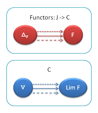
In category theory, when we say one category is “like” another category, we usually mean that there is a mapping between the two. For this mapping to be meaningful, it should preserve the structure of the category. So not only every object from one category has to be mapped into an object from another category, but also all morphisms must be mapped correctly — meaning they should preserve composition. Such a mapping has a name: it’s called a functor.

Functors in Hask are described by the type class Functor

class Functor f where
fmap :: (a -> b) -> (f a -> f b)

A Haskell Functor maps types into types and functions into functions — a type constructor does the former and fmap does the latter.

A type contructor is a mapping from one type to another. For instance, a list type constructor takes any type a and creates a list type, [a].

So instead of asking if every category is “like” the Set category, we can ask a more precise question: For what types of categories (if not all of them) there exist functors that map them into Set . Such categories are called representable, meaning they have a representation in Set .

As a physicist I had to deal a lot with groups, such as groups of spacetime rotations in various dimensions or unitary groups in complex spaces. It was very handy to represent these abstract groups as matrices acting on vectors. For instance, different representations of the same Lorenz group (more precisely, SL(2, C)) would correspond to physical particles with different spins. So vector spaces and matrices are to abstract groups as sets and functions are to abstract categories.

Yoneda Embedding

One of the things Yoneda showed is that there is at least one canonical functor from any so called locally small category into the category of sets and functions. The construction of this functor is surpisingly easy, so let me sketch it.

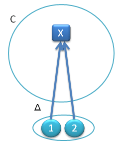
This functor should map every object in category C into a set. Set of what? It doesn’t really matter, a set is a set. So how about using a set of morphisms?

Fig 3. The Yoneda embedding. Object X is mapped by the functor into the set H_A(X). The elements of the set correspond to morphisms from A to X.

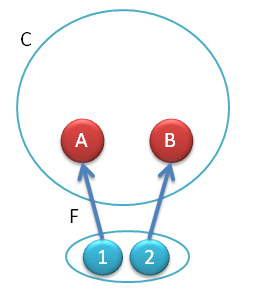
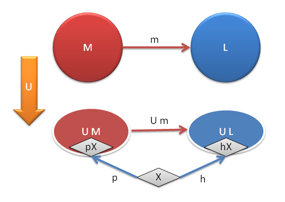
How can we map any object into a set of morphisms? Easy. First, let’s arbitrarily fix one object in the category C, call it A. It doesn’t matter which object we pick, we’ll just have to hold on to it. Now, for every object X in C there is a set of morphisms (arrows) going from our fixed A to this X. We designate this set to be the image of X under the functor we are constructing. Let’s call this functor H_A. There is one element in the set H_A(X) for every morphism from A to X.

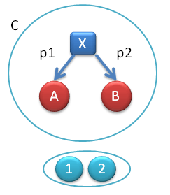
A functor must define a mapping of objects to objects (to sets, in our case) and morphisms to morphisms (to functions in our case). We have established the first part of the mapping. To define the second part, let’s pick an arbitrary morphism f from X to Y. We have to map it to some function from the set H_A(X) to the set H_A(Y).

Fig 4. The Yoneda functor also maps morphisms. Here, morphism f is mapped into the function H_A(f) between sets H_A(X) and H_A(Y).

Let’s define this function, we’ll call it H_A(f), through its action on any element of the set H_A(X), call it x. By our construction, x corresponds to some particular morphism, u, from A to X. We now have at our disposal two morphisms, u :: A -> X and f :: X -> Y (that’s the morphism we are mapping). We can compose them. The result f . u is a morphism from A to Y, so it’s a member of the set H_A(Y). We have just defined a function that takes an x from H_A(X) and maps it into y from H_A(Y), and this will be our H_A(f).

Of course, you have to prove that this construction of H_A is indeed a functor preserving composition of morphisms, but that’s reasonably easy, once the technique we have just used becomes familiar to you. Here’s the gist of this technique: Use components! When you are defining a functor from category C to category D, pick a component — an object X in C — and define its image, F(X). Then pick a morphism f in C, say from X to Y, and define its image, F(f), as a particular morphism from F(X) to F(Y).

Similarly, when defining a function from set S to T, use its components. Pick an element x of S and define its image in T. That’s exactly what we did in our construction.

Incidentally, what was that requirement that the category C be locally small? A category is locally small if the collection of morphisms between any two objects forms a set. This may come as a surprise but there are things in mathematics that are too big to be sets. A classic example is a collection of all sets, which cannot be a set itself, because it would lead to a paradox. A collection of all sets, however, is the basis of the Set category (which, incidentally, turns out to be locally small).

Summary So Far

Let me summarize what we’ve learned so far. A category is just a bunch of abstract objects and arrows between them. It tells us nothing about the internal structure of objects. However, for every (locally small) category there is a structure-preserving mapping (a functor) that maps it into a category of sets. Objects in the Set category do have internal structure: they have elements; and morphisms are functions acting on those elements. A representation maps the categorie’s surface structure of morphisms into the internal structure of sets.

It is like figuring out the properties of orbitals in atoms by looking at the chemical compounds they form, and at the way valencies work. Or discovering that baryons are composed of quarks by looking at their decay products. Incidentally, no one has ever “seen” a free quark, they always live inside other particles. It’s as if physicists were studying the “category” of baryons by mapping them into sets of quarks.

A Bar Example

This is all nice but we need an example. Let’s start with “A mathematician walks into a bar and orders a category.” The barman says, “We have this new tasty category but we can’t figure out what’s in it. All we know is that it has just one object A” — (“Oh, it’s a monoid,” the mathematician murmurs knowingly) — “…plus a whole bunch of morphisms. Of course all these morphisms go from A to A, because there’s nowhere else to go.”

What the barman doesn’t know is that the new category is just a re-packaging of the good old set of ASCII strings. The morphisms correspond to appending strings. So there is a morphism called foo that apends the string "foo"

foo :: String -> String
foo = (++"foo")

main = putStrLn $ foo "Hello "

and so on.

“I can tell you what’s inside A,” says the mathematician, “but only up to an isomorphism. I’m a mathematician not a magician.”

She quickly constructs a set that contains one element for each morphism — morphisms must, by law, be listed by the manufacturer on the label. So, when she sees foo, she puts an element with the label “foo”, and so on. Incidentally, there is one morphism with no name, which the mathematician maps to an empty label. (In reality this is an identity morphism that appends an empty string.)

“That’s what’s inside the object A,” she says.

“Moreover, this set comes equipped with functions that rearrange its elements. In fact there is a function for every morphism listed in the category,” she says. “Name any morphism and I’ll construct you a function.”

The barman gives her morphism p, which in reality is:

p = (++"p")

“Okay,” she says, “here’s how I construct the corresponding function. Pick any element in my set.”

The barman picks “foo”.

“Okay, ‘foo’ corresponds to the morphism foo,” she says, “so tell me what you call the morphism that’s the composition of foo and p?” (By law, the manufacturer is obliged to specify all admissible compositions of morphisms on the label.)

“It’s called foop,” says the barman.

Quick check:

p . foo == (++"p") . (++"foo") == (++"foop")
foop = (++"foop")

“Okay,” she says, “the function corresponding to p maps “foo” into “foop”. Hm, how curious! I bet this function will map the no-label elment into “p”, is that right?”

“Indeed, it does,” says the barman.

Quick check:

p . id == p

“I bet you this is just a string monoid,” says the mathematician.

“I think I’ll have my usual Top on the rocks instead.”

Natural Transformations

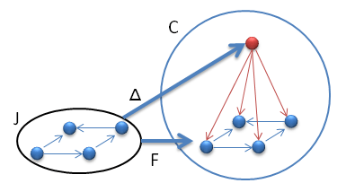
We’ve seen how to construct a representation of any (locally small) category in Set by selecting an arbitrary object A in the category and studying morphisms originating at A. What if we choose a different object B instead? How different is the representation H_A from H_B? For that matter, what if we pick any functor F from C to Set ? How is it related to H_A? That’s what the Yoneda lemma is all about.

Let me start with a short recap.

A functor is a mapping between categories that preserves their structure. The structure of a category is defined by the way its morphisms compose. A functor F maps objects into objects and morphism into morphisms in such a way that if f . g = h then F(f) . F(g) = F(h).

A natural transformation is a mapping between functors that preserves the structure of the underlying categories.

Fig 5. A component of a transformation Φ at X. Φ maps functor F into functor G, Φ_X is a morphism that maps object F(X) into object G(X).

First we have to understand how to define mappings between functors. Suppose we have functors F and G, both going from category C to category D. For a given object X in C, F will map it into F(X) in D, and G will map it into G(X) in D. A mapping Φ between functors must map object F(X) to object G(X), both in category D. We know that a mapping of objects is called a morphism. So for every object X we have to provide a morphism Φ_X from F(X) to G(X). This morphism is called a component of Φ at X. Or, looking at it from a different angle, Φ is a family of morphisms parameterized by X.

An Example of Natural Transformation

Just to give you some Haskell intuition, consider functors on Hask . These are mapping of types (type constructors) such as a -> [a] or a -> Maybe a, with the corresponging mappings of morphisms (functions) defined by fmap. Recall:

class Functor f where
fmap :: (a -> b) -> (f a -> f b)

The mapping between Haskell functors is a family of functions parameterized by types. For instance, a mapping between the [] functor and the Maybe functor will map a list of a, [a] into Maybe a. Here’s an example of such a family of functions called safeHead:

safeHead :: [a] -> Maybe a
safeHead []     = Nothing
safeHead (x:xs) = Just x

A family of functions parameterized by type is nothing special: it’s called a polymorphic function. It can also be described as a function on both types and values, with a more verbose signature:

{-# LANGUAGE ExplicitForAll #-}

safeHead :: forall a . [a] -> Maybe a
safeHead []     = Nothing
safeHead (x:xs) = Just x

main = print $ safeHead ["One", "Two"]

Let’s go back to natural transformations. I have described what it means to define a transformation of functors in terms of objects, but functors also map morphism. It turns out, however, that the tranformation of morphisms is completely determined by the two functors. A morphism f from X to Y is transformed under F into F(f) and under G into G(f). G(f) must therefore be the image of F(f) under Φ. No choice here! Except that now we have two ways of going from F(X) to G(Y).

Fig 6. The naturality square. Φ is a natural transformation if this diagram commutes, that is, both paths are equivalent.

We can first use the morphism F(f) to take us to F(Y) and then use Φ_Y to get to G(Y). Or we can first take Φ_X to take us to G(X), and then G(f) to get to G(Y). We call Φ a natural transformation if these two paths result in the same morphism (the diagram commutes).

The best insight I can offer is that a natural transformation works on structure, while a general morphism works on contents. The naturality condition ensures that it doesn’t matter if you first rearrange the structure and then the content, or the other way around. Or, in other words, that a natural transformation doesn’t touch the content. This will become clearer in examples.

Going back to Haskell: Is safeHead a natural transformation between two functors [] and Maybe? Let’s start with a function f from some type a to b. There are two ways of mapping this function: one using the fmap defined by [], which is the list function map; and the other using the Maybe‘s fmap, which is defined in the Maybe‘s functor instance definition:

instance Functor Maybe where
   fmap f (Just x) = Just (f x)
   fmap _ Nothing  = Nothing

The two path from [a] to Maybe b are:

Apply fmap f to [a] to get [b] and then safeHead it, or
Apply safeHead to [a] and then use the Maybe version of fmap.

There are only two cases to consider: an empty list and a non-empty list. For an emtpy list we get Nothing both ways, otherwise we get Just f acting on the first element of the list.

We have thus shown that safeHead is a natural transformation. There are more interestig examples of natural transformations in Haskell; monadic return and join come to mind.

The intuition behind natural transformations is that they deal with structure, not contents. safeHead couldn’t care less about what’s stored in a list, but it understands the structure of the list: things like the list being empty, or having a first element. The type of this element doesn’t matter. In Haskell, natural transformations are polymorphic functions that can, like safeHead be typed using forall:

safeHead :: forall a . [a] -> Maybe a

Yoneda Lemma

Going back to the Yoneda lemma, it states that for any functor from C to Set there is a natural transformation from our canonical representation H_A to this functor. Moreover, there are exactly as many such natural transformations as there are elements in F(A).

That, by the way, answers our other question about the dependence on the choice of A in the Yoneda embedding. The Yoneda lemma tells us that there are natural transformations both ways between H_A and H_B.

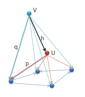
Amazingly, the proof of the Yoneda lemma, at least in one direction, is quite simple. The trick is to first define the natural transformation Φ on one special element of H_A(A): the element that corresponds to the identity morphism on A (remember, there is always one of these for every object). Let’s call this element p. Its image under Φ_A will be in F(A), which is a set. You can pick any element of this set and it will define a different but equally good Φ. Let’s call this element q. So we have fixed Φ_A(p) = q.

Now we have to define the action of Φ on an arbitrary element in the image of H_A. Remember that the functor H_A transforms objects in C into sets. So let’s take an arbitrary object X and its image H_A(X). The elements in H_A(X) correspond to morphisms from A to X. So let’s pick one such morphism and call it f. Its image is an element r in H_A(X). The question is, what does r map into under Φ? Remember, it’s image must be an element of F(X).

Fig 7. The mappings in the Yoneda lemma. F is an arbitrary functor. Any choice of p determines the morphism Φ_X for any X.

To figure that out, let’s consider the F route. F being a functor transforms our morphism f into F(f) — which is a morphism from F(A) to F(X). But, as you may remember, we have selected a special element in F(A) — our q. Now apply F(f) to q and you get an element in F(X), call it s. (Remember, F(f) is just a regular function between two sets, F(A) and F(X).)

There’s nothing more natural than picking Φ_X(r) to be this s! We have thus defined a natural transformation Φ for any X and r.

The straightforward proof that this definition of Φ is indeed natural is left as an exercise to the user.

A Haskell Example

I’ve been very meticulous about distinguishing between morphisms from A to X in C and the corresponding set elements in H_A(X). But in practice it’s more convenient to skip the middle man and define natural transformations in the Yoneda lemma as going directly from these morphisms to F(X). Keeping this in mind, the Haskell version of the Yoneda lemma is ofter written as follows:

forall r . ((a -> r) -> f r) ~ f a

where the (lowercase) f is the functor (think of it as a type constructor and its corresponding fmap), (a -> r) is a function corresponding to the morphism from A to X in our orginal formulation. The Yoneda’s natural transformation maps this morphism into the image of r under f — the F(X) in the original formulation. The forall r means that the function ((a -> r) -> f r) works for any type r, as is necessary to make it a natural transformation.

The lemma states that the type of this function, forall r . ((a -> r) -> f r) is equivalent to the much simpler type f a. If you remember that types are just sets of values, you can interpret this result as stating that there is one-to-one correspondence between natural transformations and values of the type f r.

Remember the example from the beginning of this article? There was a function imager with the following signature:

imager :: forall r . ((Bool -> r) -> [r])

This looks very much like a natural transformation from the Yoneda lemma with the type a fixed to Bool and the functor, the list functor []. (I’ll call the functions Bool->r iffies.)

The question was, how many different implementations of this signature are there?

The Yoneda lemma tells us exactly how to construct such natural transformations. It instructs us to start with an identity iffie: idBool :: Bool -> Bool, and pick any element of [Bool] to be its image under our natural transformation. We can, for instance, pick [True, False, True, True]. Once we’ve done that, the action of this natural transformation on any iffie h is fixed. We just map the morphism h using the functor (in Haskell we fmap the iffie), and apply it to our pick, [True, False, True, True].

Therefore, all natural transformations with the signature:

forall r . ((Bool -> r) -> [r])

are in one-to-one correspondence with different lists of Bool.

Conversely, if you want to find out what list of Bool is hidden in a given implementation of imager, just pass it an identity iffie. Try it:

{-# LANGUAGE ExplicitForAll #-}

imager :: forall r . ((Bool -> r) -> [r])
imager iffie = fmap iffie [True, False, True, True]

data Color = Red | Green | Blue        deriving Show
data Note  = C | D | E | F | G | A | B deriving Show

colorMap x = if x then Blue else Red
heatMap  x = if x then 32   else 212
soundMap x = if x then C    else G
idBool :: Bool -> Bool
idBool x = x

main = print $ imager idBool

Remember, this application of the Yoneda lemma is only valid if imager is a natural transformation — its naturality square must commute. The two functors in the imager naturality diagram are the Yoneda embedding and the list functor. Naturality of imager translates into the requirement that any function f :: a -> b modifying an iffie could be pulled out of the imager:

imager (f . iffie) == map f (imager iffie)

Here’s an example of such a function translating colors to strings commuting with the application of imager:

{-# LANGUAGE ExplicitForAll #-}

imager :: forall r . ((Bool -> r) -> [r])
imager iffie = fmap iffie [True, False, True, True]

data Color = Red | Green | Blue  deriving Show

colorMap x = if x then Blue else Red

f :: Color -> String
f = show 

main = do
    print $ imager (f . colorMap)
    print $ map f (imager colorMap)

The Structure of Natural Transformations

That brings another important intuition about the Yoneda lemma in Haskell. You start with a type signature that describes a natural transformation: a particular kind of polymorphic function that takes a probing function as an argument and returns a type that’s the result of a functor acting on the result type of the probing function. Yoneda tells us that the structure of this natural transformation is tightly constrained.

One of the strengths of Haskell is its very strict and powerful type system. Many Haskell programers start designing their programs by defining type signatures of major functions. The Yoneda lemma tells us that type signatures not only restrict how functions can be combined, but also how they can be implemented.

As an extreme, there is one particular signature that has only one implementation: a->a (or, more explicitly, forall a. a -> a). The only natural implementation of this signature is the identity function, id.

Just for fun, let me sketch the proof using the Yoneda lemma. If we pick the source type as the singleton unit type, (), then the Yoneda embedding consists of all functions taking unit as an argument. A function taking unit has only one return value so it’s really equivalent to this value. The functor we pick is the identity functor. So the question is, how many natural tranformation of the the following type are there?

forall a. ((() -> a) -> a)

Well, there are as many as there are elements in the image of () under the identity functor, which is exactly one! Since a function ()->a can be identified with a, it means we have only one natural transformation with the following signature:

forall a. (a -> a)

Moreover, by Yoneda construction, this function is defined by fmapping the function ()->a over the element () using the identity functor. So our natural transformation, when probed with a value of the type a will return the same value. But that’s just the definition of the identity function. (In reality things are slightly more complicated because every Haskell type must include undefined, but that’s a different story.)

Here’s an exercise for the reader: Show that the naturality square for this example is equivalent to id commuting with any function: f . id == id . f.

Conclusion

I hope I provided you with enough background information and intuition so that you’ll be able to easily read more advanced blog posts, like this one:
Reverse Engineering Machines with the Yoneda Lemma by Dan Piponi, or GADTs by Gabriel Gonzales.

Acknowledgments

I’d like to thank Gabriel Gonzales for providing useful comments and John Wiegley, Michael Sloan, and Eric Niebler for many interesting conversations.

March 17, 2011

Monads for the Curious Programmer: Part 3

Posted by Bartosz Milewski under C++, Category Theory, Functional Programming, Haskell, Type System
[10] Comments

In the previous installment I introduced monads using two examples: the Maybe monad and the List monad. Admittedly, those weren’t the most exciting uses of monads, although they served the purpose of explaining the underlying theory. I also mentioned that monads were introduced into functional programming as a general solution for a variety of problems. One of those problems was representing stateful computations as functions.

Functions, State, and Side Effects

Here’s the problem: In functional languages, every time you call a function with the same arguments, it must return the same result. In fact, if the compiler detects such a situation, it is free to memoize the result of the first call and skip subsequent calls altogether. A stateful computation, on the other hand, might return different results every time it’s performed. It may, for instance, access some global or static variables. It may also modify those variables– in other words have side effects. In extreme cases a computation might be performed purely for side effects and not even bother to return any results.

This kind of behavior is often troublesome even in imperative programming. The use of global variables in particular is being discouraged. A better solution is to encapsulate the state and pass it explicitly to functions that use it. As a syntactic shortcut, in object-oriented languages, some of the state is regularly passed to functions (methods) as a hidden “this” or “self” argument. There’s even a syntax for composing such functions, as in this JavaScript snippet:

with(document) {
    var t = title;
    write(t + " and more");
}

Here, title is a property and write a method of the object document. (If you put on your monadic glasses, it almost looks like do notation.)

In functional languages we have one more limitation: we cannot mutate any data. There’s a standard way to overcome this limitation: Instead of modifying the data, you create a modified copy. This doesn’t even have to be expensive, if the language supports smart data structures that silently substitute references for copies whenever possible. Most operations on lists in Haskell are optimized this way, and there’s even a language, Clojure, at whose core are “persistent” data structures that behave as if they were immutable, but do a lot of sharing behind the scenes. Immutability is a very attractive feature when you are doing concurrent programming: access to immutable data requires no synchronization.

Taking all this into account, the way to translate stateful computations into functional language is to use functions that explicitly take state (encapsulated in some data structure) and return the, possibly modified, state together with the usual return value. For instance, a C++ “function”:

int pop() {
    auto v = glob.top();
    glob.pop();
    return v;
}

that operates on a global vector, glob of the type std::vector<int>, would be turned into a Haskell function:

pop (ST lst) = (ST (tail lst), head lst)

operating on the state of type Stack:

newtype Stack = ST [Int]

The constructor ST creates a Stack from a list of integers. This constructor is also used for pattern matching, as in the argument of pop. The function head returns the first element of a list, tail returns the rest.

The signature of pop is characteristic of functions that operate on state:

top:: Stack-> (Stack, Int)

Such functions are often called “actions.”

There are two problems with this scheme: (1) It’s awkward, and (2) It doesn’t fit our monadic approach. In this example, the original computation (as expressed in C++) takes no arguments and returns an integer. Its functional counterpart takes a state and returns an integer combined with the state. It’s not clear how one would bind such functions together and use the convenient do notation.

We are on the right track though. We just need to get even more general: We need to separate the construction of an action from its execution. Our basic blocks will be functions that return actions– we’ll call them “monadic functions.” Since action is a function, we’ll be dealing with functions returning functions; or higher order functions.

Our goal is to find a way to compose monadic functions into larger monadic functions. A composite monadic function will return a composite action. We will then execute such action on a state, and get our result.

This new description fits the monadic pattern much better. We start with a generic stateful computation that takes an argument of type a and returns a value of type b, and we turn it into a (monadic) function that takes type a and returns an enriched type based on b. This time, though, the enriched type is a function type– an action. In general, an action is a function that takes a state (of some type S) and returns a tuple consisting of the (possibly modified) state and the value of type b.

S -> (S, b)

Here’s the first element of the monad– a type constructor: For any type t it defines a new type: an action to calculate a value of type t given a state. This type constructor is part of the state monad. Before we get to a more formal definition, let’s do some practice exercises.

The Monadic Calculator

There’s a perfect example of a stateful computation: a stack-based calculator. The state in this case is represented by the type Calc:

newtype Calc = Calc [Int]

that hides a list of integers– our calculator’s stack.

First, lets define a monadic function (a function that returns an action) that pops an element off the calculator’s stack. It will be a function returning a function, so we need to use lambdas.

popCalc = 
    \(Calc lst) -> (Calc (tail lst), head lst)

The body of the lambda is almost identical to the implementation of pop above. Notice that popCalc takes no arguments. Rather, the function that it produces takes a calculator as an argument and returns the calculator back, paired with the result–the value at the top of the stack. In other words, popCalc returns a promise to calculate the top of the calculator’s stack when the stack is available.

Here’s how you can use popCalc. First, you call it with no arguments and record the returned action. Next, you create a calculator (with a non-empty stack, otherwise the next line of code would bomb). You apply the action to that calculator and record the result– you pattern-match it to a tuple consisting of a changed calculator and a number. Finally you display that number. This is the actual output of a Haskell interpreter session:

> let f = popCalc
> let calc = Calc [3, 2, 1]
> let (calc', x) = f calc
> x
3

While we’re at it, we can similarly implement a pushCalc function:

pushCalc n =
    \(Calc lst) -> (Calc (n:lst), ())

Notice that the lambda produced by pushCalc returns a modified calculator (argument n is prepended to the list) paired with a special value () of the type unit— a Haskell equivalent of void. The imperative equivalent of this function would return void and work only through side effects. Notice also that the lambda is actually a closure: it captures the outer variable n for later use.

Finally, we need a function that performs some calculation; after all we are implementing a calculator:

addCalc =
    \(Calc lst) -> let (a:b:rest) = lst
                   in
                       (Calc ((a + b):rest), ())

Here I’m matching the calculator’s list with the pattern (a:b:rest) to retrieve the top two elements. The modified calculator has the sum of those two elements on the top of its stack.

We can use all these functions in combination to perform more complex operations, like adding two numbers. Here’s a piece code that might rival some of the Rube Goldberg creations:

add x y =
    let pux = pushCalc x -- promise to push x
        puy = pushCalc y -- promise to push y
        axy = addCalc    -- promise to add top numbers
        pp = popCalc     -- promise to pop the result
        calc = Calc []   -- we need a calculator
        (calc1, _) = pux calc  -- actually push x
        (calc2, _) = puy calc1 -- actually push y
        (calc3, _) = axy calc2 -- actually add top numbers
        (_, z) = pp calc3      -- actually pop the result
    in
        z  -- return the result

But what we really want is to be able to combine smaller actions into larger actions. For that we have to define bind. The signature of bind, in this case, should be:

bind :: (Calc -> (Calc, a)) ->        -- action
        (a -> (Calc -> (Calc, b)) ->  -- continuation
        (Calc -> (Calc, b))           -- new action

I have highlighted our enriched types–the action types. This signature looks much more complex than the signature of the Maybe bind, but that’s only because the enriched type is itself a function type. Other than that, the structure is the same: bind accepts an action and a continuation and returns a new action. The continuation in this case takes an argument of type a (the value to be calculated by the first action) and returns the composite action.

In fact, if we define Action as a type alias:

type Action a = Calc -> (Calc, a)

the signature of bind can be abbreviated to:

bind :: (Action a) -> (a -> (Action b)) ->  (Action b)

Now for the implementation. Since the result of bind is an action, it has to return a lambda of the appropriate signature.

bind act cont =
    \calc -> ... produce (Calc, b) tuple ...

Bind is supposed to compose the action, act, with the continuation, cont. So it should first apply act to calc.

let (calc', v) = act calc

The result is a tuple (calc', v) with a new calculator and a value v of type a.

This is the v that the continuation expects, so the next step is to apply the continuation:

act' = cont v

The result of the continuation is a new action. This new action can then be executed, that is applied to the new calculator:

act' calc'

to produce the desired result– a tuple of the type (Calc, b).

Here’s the final code:

bind act cont =
    \calc ->
        let (calc', v) = act calc
            act' = cont v
        in
            act' calc'

To complete our construction of the monad, we need to define return. The signature of return is:

return :: a -> Action a

and the implementation is pretty straightforward. It takes a value v and returns a promise to return this value.

return v = \calc -> (calc, v)

An astute reader might notice that nothing in this construction depends on the peculiarities of the type Calc. It will work for any type that is used to represent state. So we have in fact just constructed a generic state monad. The stack-based calculator is just a silly example of that monad.

It’s not difficult to implement bind as an infix operator, >>=, and turn the calculator into a monad that’s recognizable by the Haskell compiler (see Appendix 1). Then the relevant part of the add function may be rewritten in the do notation:

add x y = do
    pushCalc x
    pushCalc y
    addCalc
    r <- popCalc
    return r

Let me present the same code without any syntactic sugar, using the cascading lambda-within-lambda notation:

add x y =
  bind (pushCalc x) 
       (\() -> bind (pushCalc y)
                    (\() -> bind addCalc
                                 (\() -> bind popCalc
                                              (\z -> return z))))

This is not something you will see often in Haskell programs, but I will eventually want to go beyond Haskell. My goal is to connect back with C++, and this is the form that’s most convenient form making such a transition.

So let’s painstakingly analyze this code. We are binding the first action, (pushCalc x), to the rest of the code. The rest of the code is expressed as one huge lambda. To make these two parts fit together, their types have to match. The value produced by the action pushCalc is void (a.k.a., “unit”)– so it’s type is Action (). Therefore the lambda to which it binds must also take void, hence the notation:

\() -> ...

The body of that lambda is another bind, and so on, until we get to the interesting part, which is popCalc.

popCalc is an action that calculates a value: its signature is Action Int. This value is passed to the lambda to which popCalc is bound. Therefore this last lambda takes an Int argument, z. Finally, this value is enclosed in an action, and that’s done by the function return.

This unsugared notation elucidates one more aspect of the monadic approach that’s very relevant in the context of Haskell. Haskell is a lazy language: it doesn’t evaluate anything unless it is strictly necessary for achieving some final goal. Also, when it needs to evaluate several independent things, it will do that in some arbitrary, unpredictable order. So if it were somehow possible to implement the imperative versions of push and pop in Haskell, we would have two problems: push would never be evaluated because it produces no result, and even if it were, its evaluation could be swapped with the subsequent pop. Monadic bind forces the ordered evaluation of actions by introducing explicit data dependency. If pop follows push in the chain of binds, pop cannot be evaluated before push because its argument is the calculator that is returned by push. The two are linked by data dependency which, by the way, is not so obvious in the do notation.

Conclusion

The state monad is a very interesting pattern from the programming point of view. Instead of doing something, you create an action that is executed (maybe even multiple times) later. The monadic scaffolding provides the standard amenities like the ability to compose actions, and the do notation makes writing functions that produce functions much more natural. There is an interesting variation of the state monad called the IO monad, which is used for input and output in Haskell. I describe it in Appendix 2.

There are many patterns in imperative languages that have elements, or sometimes just hints, of a state monad. For instance, in the OO world you might encounter a very useful Command Pattern. You can “bind” command objects using the Composite Pattern. In languages that support anonymous functions and closures, like JavaScript, C# and, recently C++, you can return functions from functions directly. This might help, for instance, in dealing with inversion of control, where you return a closure as an event handler (that would be material for another series of blog posts).

But I have in mind a very specific example that I’ve been working on in C++ that fits the monadic pattern perfectly, and I’m going to write about it in the next installment of this series.

I’d like to thank Eric Niebler for valuable comments on the draft of this post.

Appendix 1

The full implementation of a stack-based calculator requires a few more Haskell tricks. First, we have to explicitly define our type constructor. I’ll call the new type Calculation, with the type constructor CL that encapsulates an action:

newtype Calculation a = CL (Calc -> (Calc, a))

Monadic functions have to return this new type, so they all wrap their actions into a Calculation.

pushCalc n =
    CL (\(Calc lst) -> (Calc (n:lst), ()))

topCalc = 
    CL (\(Calc lst) -> (Calc lst, head lst))

popCalc =
    CL (\(Calc lst) -> (Calc (tail lst), head lst))

addCalc =
    CL (\(Calc lst) -> let (a:b:rest) = lst
                       in
                           (Calc ((a + b):rest), ()))

Haskell has a built-in type class for Monads (think of a type class as a C++ concept). We have to tell Haskell that our Calculation is an instance of Monad and provide the definition of the two associated functions: bind, using infix notation, and return.

instance Monad Calculation where
    return x = 
        CL (\calc -> (calc, x))
    CL(c) >>= cont =
        CL (\calc ->
            let (calc', v) = c calc
                CL c' = cont v
            in
                c' calc')

With those definitions, our add function can be written using the do notation.

add x y = do
    pushCalc x
    pushCalc y
    addCalc
    r <- popCalc
    return r

Since we are not expecting any values to be calculated by pushCalc or addCalc, there are no left arrows accompanying them in the do notation.

Appendix 1a: The Applicative

Haskell keeps evolving and, on occasion, the changes in the language break old code. In particular the Monad class has a superclass now, called Applicative. That’s why the Monad instance for Calculation won’t compile any more, unless you explicitly add the instance for Applicative. Fortunately, the Applicative functionality can be fully implemented using the Monad interface, as in:

instance Applicative Calculation where
  pure = return
  mf <*> mx = do f <- mf
                 x <- mx
                 return (f x)

This won’t compile either, because Applicative requires Functor as its superclass. So we have to make Applicative a Functor. The simplest is to let the compiler work it out, but you have to include this line at the very top of the file:

{-# LANGUAGE DeriveFunctor #-}

and modify the definition of Calculation:

newtype Calculation a = CL (Calc -> (Calc, a))
  deriving Functor

In fact, it’s possible to implement the calculator as an Applicative, without the need for a Monad instance. But that’s a different story.

Appendix 2: The IO Monad

Strictly speaking a lazy purely functional language like Haskell cannot do any input or output. That’s because the compiler is free to memoize the result of the first call to, say, getChar and elide all subsequent calls. Calls to putChar, which don’t return anything, may be ignored altogether. This is why most functional languages cheat when it comes to I/O. But not Haskell. Monads to the rescue!

Let’s think for a moment why getChar may return different characters every time it’s called. It’s because there is a keyboard somewhere out there that changes its state. Why is it changing its state? Because there is a human who pushes the keys. Why is the human pushing the keys? Because he or she got a phone call from China that the price of rice is about to go up, so it makes sense to buy some futures. And so on… In other words there is this external world that is full of state.

What if we encapsulate that whole world in a hidden data structure and write our program as an action that operates on it? This is very similar to the state monad pattern except that here the programmer has no access to the state and cannot execute the action. The action is produced by main and passed to the system for execution. It’s the system, wink wink, that has access to “the world” and may pass it as a state argument to that action. Of course it’s all smoke and mirrors, but it successfully staves off the insanity of the external world from impinging on the purity of Haskell.

How does it work in practice? There is a monad called IO. It’s almost like a state monad, except that its type can’t be expressed in Haskell, because it would have to look something like this:

type IO a = World -> (World, a)

and we don’t know what World is. The main function in a Haskell program is a monadic IO action, usually:

main :: IO ()

with the type parameter a replaced by unit, (), (although any other type will work too).

The simplest main is just a single IO action:

main = putStrLn "Hello World!"

but in general main is a do block.

You might ask: If a Haskell program is one monadic IO action, then where does the traditional functional code go? The answer is that you can call traditional functions from anywhere in the do block. Even in my highly biased example there were several non-monadic function calls (head, tail, operator (+), etc.). Imagine a Haskell program as a tree: it’s trunk is monadic IO, and so are all the thick branches that have anything to do with I/O. But the thinner branches and leaves are your run of the mill functions that get (lazily) evaluated only when the main IO action is executed by the system.

Another interesting observation is that all functions that perform I/O have this information encoded in their type signature. Not in the type of its arguments, mind you, but in the return type. This is almost the opposite of what you see in imperative languages, where you’d have to pass some kind of I/O object (file or stream) to a procedure that performs I/O (except when that object is global, like standard input/output in C++). In Haskell, if you want your function to perform I/O, two things must happen: it must return an IO action that it internally constructs; and the action must find its way to the very top, to the main function. On the way up, it might be bound with other such actions either using bind or the do notation.

You might ask: How does Haskell make sure that all IO actions get to the top, so that the system may execute them? It doesn’t! But consider what you would have to do in order not to pass an action to the top. You’d have to explicitly ignore it, as in:

let _ = putStrLn "Don't print me!"

Ignoring things in Haskell is not a default thing.

« Previous Page — Next Page »

Category Theory

Universal Construction

Currying

Adjunction

Equilizer

The Moment of Zen

Limits

Videography

Universal Construction

Initial Object

Terminal Object

Algebras and Fixed Points

Monads and Algebras

T-Algebras

What’s a Container?

Container as Functor

Examples

Natural Transformations

The Yoneda Lemma

Where Do Containers Come From?

Pointed

Applicative

Monad

State

Conclusions

Bibliography and Acknowledgments

Free Monoid

Categorical Monoid

Universal Construction

Conclusion

Appendix: A Bonus Free Object

Yoneda on Functors

Back to Haskell

Undoing fmap

The Store Comonad and Yoneda

Conclusion

Appendix: Another Exercise

Acknowledgment

Update

Bibliography

The Essence of Algebra

The Essence of Expression

The Essence of Evaluation

F-Algebras

Initial Algebras

Catamorphisms

foldr

Conclusion

Acknowledgment

Bibliography

A Teaser Problem

Categories

Functors

Yoneda Embedding

Summary So Far

A Bar Example

Natural Transformations

An Example of Natural Transformation

Yoneda Lemma

A Haskell Example

The Structure of Natural Transformations

Conclusion

Acknowledgments

Functions, State, and Side Effects

The Monadic Calculator

Conclusion

Appendix 1

Appendix 1a: The Applicative

Appendix 2: The IO Monad

Top Posts

License

Blogroll

Follow Me

Archives