Working with double categories can be aptly summarized in a meme: Talk to me about sets without mentioning sets. We don’t talk about hom-sets, we talk about horizontal units. Secretly, we are visualizing horizontal arrows as profunctors, and the unit of profunctor composition is a hom-functor.
Presheaves are defined as 
Granted, a lot of standard categorical constructions can be generalized to use profunctors in place of presheaves, with immediate generalization to double categorical settings. This can be done with (weighted) limits, Kan extensions, categories of elements (tabulations), and many others. But sometimes you just need to talk about presheaves without mentioning presheaves.
I will first sketch the constructions in category theory and, in the next installment, show you a toy implementation in Haskell.
Overview
To translate the Yoneda construction into the language of double categories, we need to define an object (a 0-cell) 

![\hat A = [A, \mathbf{Set}]](https://s0.wp.com/latex.php?latex=%5Chat+A+%3D+%5BA%2C+%5Cmathbf%7BSet%7D%5D&bg=ffffff&fg=29303b&s=0&c=20201002)

Since in this picuture the 0-cells of a double category represent categories, with no access to their objects, we have to define everything using universal constructions.
Even the simplest thing, like the action of a presheaf on an object resulting in a set, has to be defined in bulk, as a particular horizontal arrow from 
We would also like the Yoneda embedding to be dense– a generalization of the slogan that every presheaf is a colimit of representables. We can express this in terms of left Kan extensions, which we know how to generalize to double categories.
Finally, we want the Yoneda embedding to be full and faithful, without talking about the mapping of hom-sets.
Most of this stuff can be expressed using 2-cells, which we can visualize using string diagrams. The problem is that a 2-cell translates into a one-way mapping, from left to right. What we often need is isomorphisms, which require some 2-cells to be invertible.
Classifying Arrows
It’s easy to turn a functor into a profunctor. In fact there are two canonical ways of defining representable profunctors. In a proarrow equipment they correspond to the companion and the conjoint, 

The rough idea is that a profunctor:

when curried, can be seen as a functor into the presheaf category:


(Koudenburg calls this functor 

(In what follows, I’ll sometimes omit the subscript 
In components, this equivalence can be written as an invertible natural transformation:

There is one more detail that requires special attention: 


![\hat A = [C^{op}, \mathbf{Set}]](https://s0.wp.com/latex.php?latex=%5Chat+A+%3D+%5BC%5E%7Bop%7D%2C+%5Cmathbf%7BSet%7D%5D&bg=ffffff&fg=29303b&s=0&c=20201002)
is a functor category. We don’t think twice about applying functors to objects. But what it really means is that we are using the counit of the currying adjunction, the evaluation (pro-)functor:

The currying of the profunctor

One direction, left to right, of this identity can be illustrated as a double-categorical 2-cell:
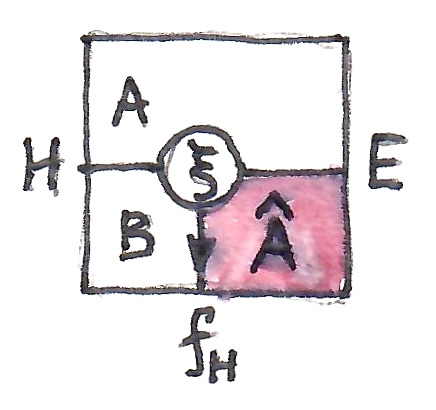
We get the other direction by requiring this square to be cartesian (see Appendix 1).
The pair 

Yoneda Embedding
We can now ask the question: What is the classifying arrow for the simplest horizontal arrow: the unit arrow? In 

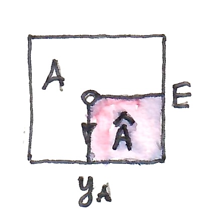
evaluates to:

or, expanding 

Compare this with the definition of the Yoneda embedding:
You may also recognize this 2-cell as a definition of the unit of a companion. Thus, in a proarrow equipment, the evaluation profunctor can be seen as a companion to the Yoneda functor:

The terse notation for the companion of a functor 


With this definition of 
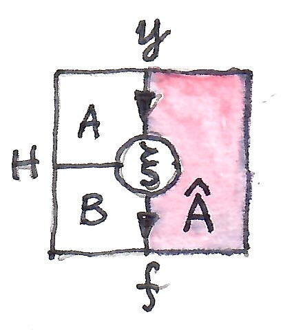
To generalize the condition that every presheaf is a colimit of representables, we want
A functor is dense if its left Kan extension along itself (called the density comonad) is isomorphic to identity:

The Adjunction
In a proarrow equipment, the counit of the companion is a 2-cell:

with 

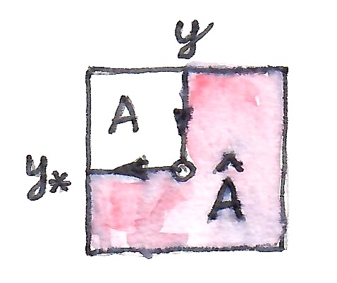
In
, \hat F)](https://s0.wp.com/latex.php?latex=%5Chat+F+a+%5Cto+%5BA%2C+%5Cmathbf%7BSet%7D%5D%28A%28-%2C+a%29%2C+%5Chat+F%29&bg=ffffff&fg=29303b&s=0&c=20201002)
Observe that this is half of the Yoneda lemma. In general, the other half– right to left– doesn’t automatically hold in an equipment.
In an equipment, the conjoint is the left adjoint of the companion. In the case of the Yoneda arrow, the adjunction reads:

where 
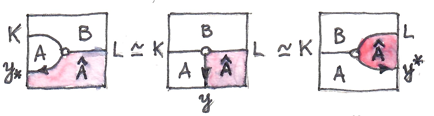
with 

The unit of this adjunction is generated by replacing 
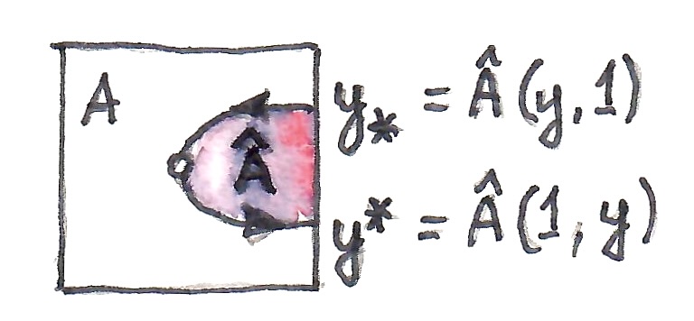
Thus the unit provides us with the one-way mapping:

or, in expanded notation:

In a proarrow equipment, we can straighten the two arrows to get the 2-cell:
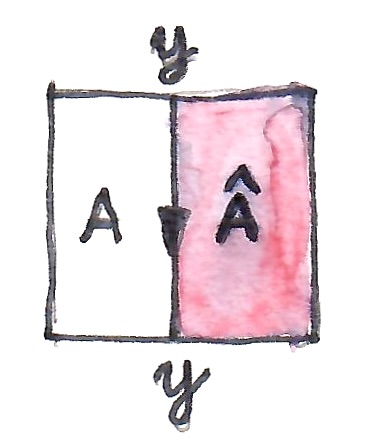
This is interpreted as a mapping from the unit arrow (horizontal-, thus elided) in
, A(-, a'))](https://s0.wp.com/latex.php?latex=A%28a%2C+a%27%29+%5Ccong+%5Chat+A+%28y+a%2C+y+a%27%29+%3D+%5BA%2C+%5Cmathbf%7BSet%7D%5D%28A%28-%2C+a%29%2C+A%28-%2C+a%27%29%29&bg=ffffff&fg=29303b&s=0&c=20201002)
which is the usual proof that the Yoneda embedding is fully faithful.
This is not an isomorphism in an arbitrary equipment, though.
We will therefore impose the condition that the unit of the adjunction
I’m grateful to John Baez for constructive criticism.
Appendix 1
The currying condition tells us that for any 0-cell 


In genereal, this doesn’t nail things down enough. There may be many candidates for
What we want is to be able to reconstruct

This can be accomplished by requiring that the above 2-cell be a cartesian square. A cartesian square is defined by a universal condition with a trio of probes 
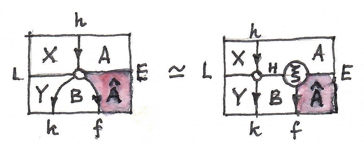
This might seem like a lot to process, but there is a trick to it. In 


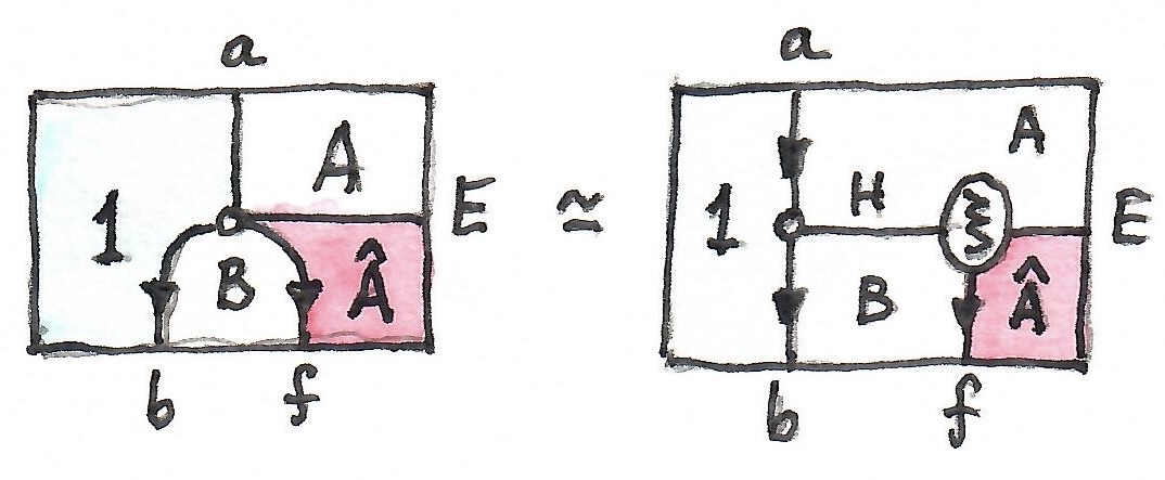
The left hand side is a mapping 


In a general double category we might not have a terminal 0-cell to select global elements, so we use the next best thing: generalized elements given by the trio

 arrow, replacing it with its horizontal conjoint
  . In a profunctor equipment, this is just a representable profunctor
  .
.  .
. 
 of the shape below can be uniquely factorized through the counit
  :
:


 along a horizontal 1-cell

 , with functors as morphisms.
 . In fact, profunctors can be considered arrows in the category
  . Not only that,
 then
then  .
. is the identity profunctor with respect to this composition. It means that we have a way of talking about hom-sets and representables without peeking inside individual categories.
 and
and  with two (horizontal) profunctors
  and
and  .
. 
 is a function:

 is sometimes called the restriction of
  .
.
 , in diagram order).


 with the appropriate injection into the coend.
 implementing the functoriality of
  or
or 
 or
or  , is defined in
 (the same as
 stands for comPanion):

 .
.

 is the identity at


 :
:


 . Or we can consider a simpler case of the double category of sets and relations. We can also add more structure to the categories in question, for instance by considering monoidal categories; or even go meta, and study the double category of (weak) double categories
  .
.