Pointwise Kan Extensions

In my category theory blog posts, I stated many theorems, but I didn’t provide many proofs. In most cases, it’s enough to know that the proof exists. We trust mathematicians to do their job. Granted, when you’re a professional mathematician, you have to study proofs, because one day you’ll have to prove something, and it helps to know the tricks that other people used before you. But programmers are engineers, and are therefore used to taking advantage of existing solutions, trusting that somebody else made sure they were correct. So it would seem that mathematical proofs are irrelevant to programming. Or so it may seem, until you learn about the Curry-Howard isomorphism–or propositions as types, as it is sometimes called–which says that there is a one to one correspondence between logic and programs, and that every function can be seen as a proof of a theorem. And indeed, I found that a lot of proofs in category theory turn out to be recipes for implementing functions. In most cases the problem can be reduced to this: Given some morphisms, implement another morphism, usually using simple composition. This is very much like using point-free notation to define functions in Haskell. The other ingredient in categorical proofs is diagram chasing, which is very much like equational resoning in Haskell. Of course, mathematicians use different notation, and they use lots of different categories, but the principles are the same.

I want to illustrate these points with the example from Emily Riehl’s excellent book Category Theory in Context. It’s a book for mathematicians, so it’s not an easy read. I’m going to concentrate on theorem 6.2.1, which derives a formula for left Kan extensions using colimits. I picked this theorem because it has calculational content: it tells you how to calculate a particular functor.

It’s not a short proof, and I have made it even longer by unpacking every single step. These steps are not too hard, it’s mostly a matter of understanding and using definitions of functoriality, naturality, and universality.

There is a bonus at the end of this post for Haskell programmers.

Kan Extensions

I wrote about Kan extensions before, so here I’ll only recap the definition using the notation from Emily’s book. Here’s the setup: We want to extend a functor $F$ , which goes from category $C$ to $E$ , along another functor $K$ , which goes from $C$ to $D$ . This extension is a new functor from $D$ to $E$ .

To give you some intuition, imagine that the functor $F$ is the Rosetta Stone. It’s a functor that maps the Ancient Egyptian text of a royal decree to the same text written in Ancient Greek. The functor $K$ embeds the Rosetta Stone hieroglyphics into the know corpus of Egyptian texts from various papyri and inscriptions on the walls of temples. We want to extend the functor $F$ to the whole corpus. In other words, we want to translate new texts from Egyptian to Greek (or whatever other language that’s isomorphic to it).

In the ideal case, we would just want $F$ to be isomorphic to the composition of the new functor after $K$ . That’s usually not possible, so we’ll settle for less. A Kan extension is a functor which, when composed with $K$ produces something that is related to $F$ through a natural transformation. In particular, the left Kan extension, $Lan_K F$ , is equipped with a natural transformation $\eta$ from $F$ to $Lan_K F \circ K$ .

(The right Kan extension has this natural transformation reversed.)

There are usually many such functors, so there is the standard trick of universal construction to pick the best one.

In our analogy, we would ideally like the new functor, when applied to the hieroglyphs from the Rosetta stone, to exactly reproduce the original translation, but we’ll settle for something that has the same meaning. We’ll try to translate new hieroglyphs by looking at their relationship with known hieroglyphs. That means we should look closely at morphism in $D$ .

Comma Category

The key to understanding how Kan extensions work is to realize that, in general, the functor $K$ embeds $C$ in $D$ in a lossy way.

There may be objects (and morphisms) in $D$ that are not in the image of $K$ . We have to somehow define the action of $Lan_K F$ on those objects. What do we know about such objects?

We know from the Yoneda lemma that all the information about an object is encoded in the totality of morphisms incoming to or outgoing from that object. We can summarize this information in the form of a functor, the hom-functor. Or we can define a category based on this information. This category is called the slice category. Its objects are morphisms from the original category. Notice that this is different from Yoneda, where we talked about sets of morphisms — the hom-sets. Here we treat individual morphisms as objects.

This is the definition: Given a category $C$ and a fixed object $c$ in it, the slice category $C/c$ has as objects pairs $(x, f)$ , where $x$ is an object of $C$ and $f$ is a morphism from $x$ to $c$ . In other words, all the arrows whose codomain is $c$ become objects in $C/c$ .

A morphism in $C/c$ between two objects, $(x, f)$ and $(y, g)$ is a morphism $h : x \to y$ in $C$ that makes the following triangle commute:

In our case, we are interested in an object $d$ in $D$ , and the slice category $D/d$ describes it in terms of morphisms. Think of this category as a holographic picture of $d$ .

But what we are really interested in, is how to transfer this information about $d$ to $E$ . We do have a functor $F$ , which goes from $C$ to $E$ . We need to somehow back-propagate the information about $d$ to $C$ along $K$ , and then use $F$ to move it to $E$ .

So let’s try again. Instead of using all morphisms impinging on $d$ , let’s only pick the ones that originate in the image of $K$ , because only those can be back-propagated to $C$ .

This gives us limited information about $d$ , but it’ll have to do. We’ll just use a partial hologram of $d$ . Instead of the slice category, we’ll use the comma category $K \downarrow d$ .

Here’s the definition: Given a functor $K : C \to D$ and an object $d$ of $D$ , the comma category $K \downarrow d$ has as objects pairs $(c, f)$ , where $c$ is an object of $C$ and $f$ is a morphism from $K c$ to $d$ . So, indeed, this category describes the totality of morphisms coming to $d$ from the image of $K$ .

A morphism in the comma category from $(c, f)$ to $(c', g)$ is a morphism $h : c \to c'$ such that the following triangle commutes:

So how does back-propagation work? There is a projection functor $\Pi_d : K \downarrow d \to C$ that maps an object $(c, f)$ to $c$ (with obvious action on morphisms). This functor loses a lot of information about objects (completely forgets the $f$ part), but it keeps a lot of the information in morphisms — it only picks those morphisms in $C$ that preserve the structure of the comma category. And it lets us “upload” the hologram of $d$ into $C$

Next, we transport all this information to $E$ using $F$ . We get a mapping

$F \circ \Pi_d : K \downarrow d \to E$

Here’s the main observation: We can look at this functor $F \circ \Pi_d$ as a diagram in $E$ (remember, when constructing limits, diagrams are defined through functors). It’s just a bunch of objects and morphisms in $E$ that somehow approximate the image of $d$ . This holographic information was extracted by looking at morphisms impinging on $d$ . In our search for $(Lan_K F) d$ we should therefore look for an object in $E$ together with morphisms impinging on it from the diagram we’ve just constructed. In particular, we could look at cones under that diagram (or co-cones, as they are sometimes called). The best such cone defines a colimit. If that colimit exists, it is indeed the left Kan extension $(Lan_K F) d$ . That’s the theorem we are going to prove.

To prove it, we’ll have to go through several steps:

Show that the mapping we have just defined on objects is indeed a functor, that is, we’ll have to define its action on morphisms.
Construct the transformation $\eta$ from $F$ to $Lan_K F \circ K$ and show the naturality condition.
Prove universality: For any other functor $G$ together with a natural transformation $\gamma$ , show that $\gamma$ uniquely factorizes through $\eta$ .

All of these things can be shown using clever manipulations of cones and the universality of the colimit. Let’s get to work.

Functoriality

We have defined the action of $Lan_K F$ on objects of $D$ . Let’s pick a morphism $g : d \to d'$ . Just like $d$ , the object $d'$ defines its own comma category $K \downarrow d'$ , its own projection $\Pi_{d'}$ , its own diagram $F \circ \Pi_{d'}$ , and its own limiting cone. Parts of this new cone, however, can be reinterpreted as a cone for the old object $d$ . That’s because, surprisingly, the diagram $F \circ \Pi_{d'}$ contains the diagram $F \circ \Pi_{d}$ .

Take, for instance, an object $(c, f) : K \downarrow d$ , with $f: K c \to d$ . There is a corresponding object $(c, g \circ f)$ in $K \downarrow d'$ . Both get projected down to the same $c$ . That shows that every object in the diagram for the $d$ cone is automatically an object in the diagram for the $d'$ cone.

Now take a morphism $h$ from $(c, f)$ to $(c', f')$ in $K \downarrow d$ . It is also a morphism in $K \downarrow d'$ between $(c, g \circ f)$ and $(c', g \circ f')$ . The commuting triangle condition in $K \downarrow d$

$f = f' \circ K h$

ensures the commuting condition in $K \downarrow d'$

$g \circ f = g \circ f' \circ K h$

All this shows that the new cone that defines the colimit of $F \circ \Pi_{d'}$ contains a cone under $F \circ \Pi_{d}$ .

But that diagram has its own colimit $(Lan_K F) d$ . Because that colimit is universal, there must be a unique morphism from $(Lan_K F) d$ to $(Lan_K F) d'$ , which makes all triangles between the two cones commute. We pick this morphism as the lifting of our $g$ , which ensures the functoriality of $Lan_K F$ .

The commuting condition will come in handy later, so let’s spell it out. For every object $(c, f:Kc \to d)$ we have a leg of the cone, a morphism $V_d^{(c, f)}$ from $F c$ to $(Lan_K F) d$ ; and another leg of the cone $V_{d'}^{(c, g \circ f)}$ from $F c$ to $(Lan_K F) d'$ . If we denote the lifting of $g$ as $(Lan_K F) g$ then the commuting triangle is:

$(Lan_K F) g \circ V_{d}^{(c, f)} = V_{d'}^{(c, g \circ f)}$

In principle, we should also check that this newly defined functor preserves composition and identity, but this pretty much follows automatically whenever lifting is defined using composition of morphisms, which is indeed the case here.

Natural Transformation

We want to show that there is a natural transformation $\eta$ from $F$ to $Lan_K F \circ K$ . As usual, we’ll define the component of this natural transformation at some arbitrary object $c$ . It’s a morphism between $F c$ and $(Lan_K F) (K c)$ . We have lots of morphisms at our disposal, with all those cones lying around, so it shouldn’t be a problem.

First, observe that, because of the pre-composition with $K$ , we are only looking at the action of $Lan_K F$ on objects which are inside the image of $K$ .

The objects of the corresponding comma category $K \downarrow K c'$ have the form $(c, f)$ , where $f : K c \to K c'$ . In particular, we can pick $c' = c$ , and $f = id_{K c}$ , which will give us one particular vertex of the diagram $F \circ \Pi_{K c}$ . The object at this vertex is $F c$ — exactly what we need as a starting point for our natural transformation. The leg of the colimiting cone we are interested in is:

$V_{K c}^{(c, id)} : F c \to (Lan_K F) (K c)$

We’ll pick this leg as the component of our natural transformation $\eta_c$ .

What remains is to show the naturality condition. We pick a morphism $h : c \to c'$ . We know how to lift this morphism using $F$ and using $Lan_K F \circ K$ . The other two sides of the naturality square are $\eta_c$ and $\eta_{c'}$ .

The bottom left composition is $(Lan_K F) (K h) \circ V_{K c}^{(c, id)}$ . Let’s take the commuting triangle that we used to show the functoriality of $Lan_K F$ :

$(Lan_K F) g \circ V_{d}^{(c, f)} = V_{d'}^{(c, g \circ f)}$

and replace $f$ by $id_{K c}$ , $g$ by $K h$ , $d$ by $K c$ , and $d'$ by $K c'$ , to get:

$(Lan_K F) (K h) \circ V_{K c}^{(c, id)} = V_{K c'}^{(c, K h)}$

Let’s draw this as the diagonal in the naturality square, and examine the upper right composition:

$V_{K c'}^{(c', id)} \circ F h$ .

This is also equal to the diagonal $V_{K c'}^{(c, K h)}$ . That’s because these are two legs of the same colimiting cone corresponding to $(c', id_{K c'})$ and $(c, K h)$ . These vertices are connected by $h$ in $K \downarrow K c'$ .

But how do we know that $h$ is a morphism in $K \downarrow K c'$ ? Not every morphism in $C$ is a morphism in the comma category. In this case, however, the triangle identity is automatic, because one of its sides is an identity $id_{K c'}$ .

We have shown that our naturality square is composed of two commuting triangles, with $V_{K c'}^{(c, K h)}$ as its diagonal, and therefore commutes as a whole.

Universality

Kan extension is defined using a universal construction: it’s the best of all functors that extend $F$ along $K$ . It means that any other extension will factor through ours. More precisely, if there is another functor $G$ and another natural transformation:

$\gamma : F \to G \circ K$

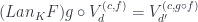
then there is a unique natural transformation $\alpha$ , such that

$(\alpha \cdot K) \circ \eta = \gamma$

(where we have a horizontal composition of a natural transformation $\alpha$ with the functor $K$ )

As always, we start by clearly stating the goals. The proof proceeds in these steps:

Implement $\alpha$ .
Prove that it’s natural.
Show that it factorizes $\gamma$ through $\eta$ .
Show that it’s unique.

We are defining a natural transformation $\alpha$ between two functors: $Lan_K F$ , which we have defined as a colimit, and $G$ . Both are functors from $D$ to $E$ . Let’s implement the component of $\alpha$ at some $d$ . It must be a morphism:

$\alpha_d : (Lan_K F) d \to G d$

Notice that $d$ varies over all of $D$ , not just the image of $K$ . We are comparing the two extensions where it really matters.

We have at our disposal the natural transformation:

$\gamma : F \to G \circ K$

or, in components:

$\gamma_c : F c \to G (K c)$

More importantly, though, we have the universal property of the colimit. If we can construct a cone with the nadir at $G d$ then we can use its factorizing morphism to define $\alpha_d$ .

This cone has to be built under the same diagram as $(Lan_K F) d$ . So let’s start with some $(c, f : K c \to d)$ . We want to construct a leg of our new cone going from $F c$ to $G d$ . We can use $\gamma_c$ to get to $G (K c)$ and then hop to $G d$ using $G f$ . Thus we can define the new cone’s leg as:

$W_c = G f \circ \gamma_c$

Let’s make sure that this is really a cone, meaning, its sides must be commuting triangles.

Let’s pick a morphism $h$ in $K \downarrow d$ from $(c, f)$ to $(c', f')$ . A morphism in $K \downarrow d$ must satisfy the triangle condition, $f = f' \circ K h$ :

We can lift this triangle using $G$ :

$G f = G f' \circ G (K h)$

Naturality condition for $\gamma$ tells us that:

$\gamma_{c'} \circ F h = G (K h) \circ \gamma_c$

By combining the two, we get the pentagon:

whose outline forms a commuting triangle:

$G f \circ \gamma_c = G f' \circ \gamma_{c'} \circ F h$

Now that we have a cone with the nadir at $G d$ , universality of the colimit tells us that there is a unique morphism from the colimiting cone to it that factorizes all triangles between the two cones. We make this morphism our $\alpha_d$ . The commuting triangles are between the legs of the colimiting cone $V_d^{(c, f)}$ and the legs of our new cone $W_c$ :

$\alpha_d \circ V_d^{(c, f)} = G f \circ \gamma_c$

Now we have to show that so defined $\alpha$ is a natural transformation. Let’s pick a morphism $g : d \to d'$ . We can lift it using $Lan_K F$ or using $G$ in order to construct the naturality square:

$G g \circ \alpha_d = \alpha_{d'} \circ (Lan_K F) g$

Remember that the lifting of a morphism by $Lan_K F$ satisfies the following commuting condition:

$(Lan_K F) g \circ V_{d}^{(c, f)} = V_{d'}^{(c, g \circ f)}$

We can combine the two diagrams:

The two arms of the large triangle can be replaced using the diagram that defines $\alpha$ , and we get:

$G (g \circ f) \circ \gamma_c = G g \circ G f \circ \gamma_c$

which commutes due to functoriality of $G$ .

Now we have to show that $\alpha$ factorizes $\gamma$ through $\eta$ . Both $\eta$ and $\gamma$ are natural transformations between functors going from $C$ to $E$ , whereas $\alpha$ connects functors from $D$ to $E$ . To extend $\alpha$ , we horizontally compose it with the identity natural transformation from $K$ to $K$ . This is called whiskering and is written as $\alpha \cdot K$ . This becomes clear when expressed in components. Let’s pick an object $c$ in $C$ . We want to show that:

$\gamma_c = \alpha_{K c} \circ \eta_c$

Let’s go back all the way to the definition of $\eta$ :

$\eta_c = V_{K c}^{(c, id)}$

where $id$ is the identity morphism at $K c$ . Compare this with the definition of $\alpha$ :

$\alpha_d \circ V_d^{(c, f)} = G f \circ \gamma_c$

If we replace $f$ with $id$ and $d$ with $K c$ , we get:

$\alpha_{K c} \circ V_{K c}^{(c, id)} = G id \circ \gamma_c$

which, due to functoriality of $G$ is exactly what we need:

$\alpha_{K c} \circ \eta_c = \gamma_c$

Finally, we have to prove the uniqueness of $\alpha$ . Here’s the trick: assume that there is another natural transformation $\alpha'$ that factorizes $\gamma$ . Let’s rewrite the naturality condition for $\alpha'$ :

$G g \circ \alpha'_d = \alpha'_{d'} \circ (Lan_K F) g$

Replacing $g : d \to d'$ with $f : K c \to d$ , we get:

$G f \circ \alpha'_{K c} = \alpha'_d \circ (Lan_K F) f$

The lifiting of $f$ by $Lan_K F$ satisfies the triangle identity:

$V_d^{(c, f)} = (Lan_K F) f \circ V_{K c}^{(c, id)}$

where we recognize $V_{K c}^{(c, id)}$ as $\eta_c$ .

We said that $\alpha'$ factorizes $\gamma$ through $\eta$ :

$\gamma_c = \alpha'_{K c} \circ \eta_c$

which let us straighten the left side of the pentagon.

This shows that $\alpha'$ is another factorization of the cone with the nadir at $G d$ through the colimit cone with the nadir $(Lan_K F) d$ . But that would contradict the universality of the colimit, therefore $\alpha'$ must be the same as $\alpha$ .

This completes the proof.

Haskell Notes

This post would not be complete if I didn’t mention a Haskell implementation of Kan extensions by Edward Kmett, which you can find in the library Data.Functor.Kan.Lan. At first look you might not recognize the definition given there:

data Lan g h a where
  Lan :: (g b -> a) -> h b -> Lan g h a

To make it more in line with the previous discussion, let’s rename some variables:

data Lan k f d where
  Lan :: (k c -> d) -> f c -> Lan k f d

This is an example of GADT syntax, which is a Haskell way of implementing existential types. It’s equivalent to the following pseudo-Haskell:

Lan k f d = exists c. (k c -> d, f c)

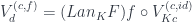
This is more like it: you may recognize (k c -> d) as an object of the comma category $K \downarrow d$ , and f c as the mapping of $c$ (which is the projection of this object back to $C$ ) under the functor $F$ . In fact, the Haskell representation is based on the encoding of the colimit using a coend:

$(Lan_K F) d = \int^{c \in C} C(K c, d) \times F c$

The Haskell library also contains the proof that Kan extension is a functor:

instance Functor (Lan k f) where
  fmap g (Lan kcd fc) = Lan (g . kcd) fc

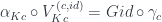
The natural transformation $\eta$ that is part of the definition of the Kan extension can be extracted from the Haskell definition:

eta :: f c -> Lan k f (k c)
eta = Lan id

In Haskell, we don’t have to prove naturality, as it is a consequence of parametricity.

The universality of the Kan extension is witnessed by the following function:

toLan :: Functor g => (forall c. f c -> g (k c)) -> Lan k f d -> g d
toLan gamma (Lan kcd fc) = fmap kcd (gamma fc)

It takes a natural transformation $\gamma$ from $F$ to $G \circ K$ , and produces a natural transformation we called $\alpha$ from $Lan_K F$ to $G$ .

This is $\gamma$ expressed as a composition of $\alpha$ and $\eta$ :

fromLan :: (forall d. Lan k f d -> g d) -> f c -> g (k c)
fromLan alpha = alpha . eta

As an example of equational reasoning, let’s prove that $\alpha$ defined by toLan indeed factorizes $\gamma$ . In other words, let’s prove that:

fromLan (toLan gamma) = gamma

Let’s plug the definition of toLan into the left hand side:

fromLan (\(Lan kcd fc) -> fmap kcd (gamma fc))

then use the definition of fromLan:

(\(Lan kcd fc) -> fmap kcd (gamma fc)) . eta

Let’s apply this to some arbitrary function g and expand eta:

(\(Lan kcd fc) -> fmap kcd (gamma fc)) (Lan id g)

Beta-reduction gives us:

fmap id (gamma g)

which is indeed equal to the right hand side acting on g:

gamma g

The proof of toLan . fromLan = id is left as an exercise to the reader (hint: you’ll have to use naturality).

Acknowledgments

I’m grateful to Emily Riehl for reviewing the draft of this post and for writing the book from which I borrowed this proof.

Sergei Winitzki Says:

January 23, 2018 at 11:00 am

Hello,
In your “Category theory” chapter 9 you say about the Curry-Howard isomorphism: “These are all interesting examples, but is there a practical side to Curry-Howard isomorphism? Probably not in everyday programming”. So maybe you will be pleased to know that last month I implemented a Scala library for generating code based on type signatures.
https://github.com/Chymyst/curryhoward

For example, you can specify a type such as (A => E => B) => (E => A) => (E => B) – (the monadic bind for the Reader monad), and the library will translate this into a formula in the intuitionistic propositional logic, find a proof term, and generate a Scala expression corresponding to that proof term. The Scala syntax looks like this:

def flatMap[E, A, B]: (E ⇒ A) ⇒ (A ⇒ E => B) ⇒ (E ⇒ B) = implement

Just to let you know, I am also participating in a book club going through all chapters of your “Category theory” book. We enjoy it, and we try to translate the code into Scala since that’s the language we use at work. Thank you for making this material available!

— Sergei

Bartosz Milewski Says:

January 24, 2018 at 4:23 am

There is a project on GitHub with Scala code for my book.

Chris Kuklewicz Says:

January 27, 2018 at 1:49 pm

I agree that “Both get projected down to the same c.” which shows {the objects in the diagram from d} are a subset of {the objects in the diagram from d’}.

Then you write “That shows that objects that form the two diagrams are indeed the same.”

I do not see how to get “same” without showing the other direction, so they they are each a subset of the other. And I can not see why {the objects in the diagram from d’} are a subset of {the objects in the diagram from d}. The direction of morphism g only makes one subset direction easy to prove.

As it happens, it is clear that the proven subset direction means that a cone (or co-cone or limit or colimit) in E derived from d’ is also a cone (or …) in E derived from d. So there is no harm to the rest of the construction.

January 28, 2018 at 9:48 am

You’re right, I got carried away. All I need for the proof is that there is a cone under $K \downarrow d$ with a nadir at $d'$ . It doesn’t have to be the same as the cone under $K \downarrow d'$ .

Jason Hooper (@jasonincanada) Says:

June 16, 2018 at 5:12 pm

Hi, I think I noticed an issue: in the fifth drawing, the object labeled “c” should really be “d”, since it’s in the category D.

June 16, 2018 at 9:49 pm

Good catch, Jason! I patched up the drawing.

(Milewski) Поточечные расширения Кана — Переводной календарь Says:

August 30, 2018 at 8:28 am

[…] Перевод статьи Бартоша Милевски «Pointwise Kan Extensions» (исходный текст расположен по адресу — Текст оригинальной статьи). […]

fufufu Says:

January 18, 2023 at 7:38 am

Hi.
I just got an issue on the formula Wc=Gf°γc i in the “universality” part.It really confuses me,since the formula has f on the right hand side but f is not fixed.
Really great article,thanks a lot.

January 18, 2023 at 8:45 am

I should have specified the pair (c, f) as parameterising W, because that’s the object of the comma category that defines the base of the cone.

Bartosz Milewski's Programming Cafe