Previously: Kan Extensions in Double Categories.
In programming, actegories play a central role in optics: lenses, prisms, traversals, etc. To understand actegories, let’s start with the definition of a monoidal category.
Monoidal Category
A monoidal category 


natural in all three arguments. We also have a unit object 

To get a better feel for it, we can try to model a monoidal category in Haskell. We parameterize it by the type of the tensor product, ten, which we want to be a Bifunctor:
class (Bifunctor ten) => MonoidalCategory ten where ...
The standard way to define a subcategory of Hask is to restrict the types of objects by imposing a constraint. Such a restriction has a special kind, Constraint:
class Bifunctor ten => MonoidalCategory (obj :: Type -> Constraint) ten where ...
A common example of such a constraint is a typeclass. For instance Monoid will restrict the objects of the category to be monoids. (In principle, we should also restrict the type of arrows, here to monoid morphisms.)
We can specify the unit of a monoidal category as an associated type (parameterized by ten):
type Unit ten :: TypeThe unit should be an object of the category, so it should satisfy the constraint. We can encode this in our definition as a precondition: obj (Unit ten). This leads to a circularity, which we can overcome using the language pragma UndecidableSuperClasses:
class (Bifunctor ten , obj (Unit ten)) => MonoidalCategory (obj :: Type -> Constraint) ten where type Unit ten :: Type ...
Finally, we can add the associator and the unitors (and their inverses):
class (Bifunctor ten , obj (Unit ten)) => MonoidalCategory (obj :: Type -> Constraint) ten where type Unit ten :: Type alpha :: (obj a, obj b, obj c) => (a `ten` b) `ten` c -> a `ten` (b `ten` c) lambda :: (obj a) => (Unit ten) `ten` a -> a ...
Notice the obj constraints in the type of these functions and the infix notation for the tensor.
Let’s work out a few examples. The simplest is the category of all types with a cartesian product as tensor.
instance MonoidalCategory Hask (,) where type Unit (,) = () alpha ((a, b), c) = (a, (b, c)) lambda ((), a) = a ...
We define Hask using an empty class, and we make all objects its instances:
class Hask ainstance Hask a
Similarly, we can define a monoidal category with Either as the tensor product, or with Monoid as the object constraint.
Actegory
An actegory is a category that supports the action of a monoidal category. You may think of it as “multiplying” or “scaling” the objects of this category by objects of the monoidal category. The (left) action can be defined as a functor from the product category to 

or, after currying, as a functor from
![\triangleright \colon \mathbf M \to [C, C]](https://s0.wp.com/latex.php?latex=%5Ctriangleright+%5Ccolon+%5Cmathbf+M+%5Cto+%5BC%2C+C%5D&bg=ffffff&fg=29303b&s=0&c=20201002)
The coherency conditions are the invertible natural transformations that relate the action 


The action is functorial in both arguments, so our Haskell translation pegs it, for simplicity, as a Bifunctor. (A Profunctor action is also possible. Categorically, it would correspond to using 
class (MonoidalCategory obj ten, Bifunctor act) => Actegory obj ten act | act -> ten where assoc :: (obj m, obj n) => (m `ten` n) `act` a -> m `act` (n `act` a) assoc' :: (obj m, obj n) => m `act` (n `act` a) -> (m `ten` n) `act` a unit :: Unit ten `act` a -> a unit' :: a -> Unit ten `act` a
Another simplifying assumption is that the action uniquely identifies the tensor product, encoded here as the functional dependency act -> ten.
The simplest example of an actegory is the self action of the cartesian product. Here, the monoidal category acts on itself:
instance Actegory Hask (,) (,) where assoc ((m, n), a) = (m, (n, a)) assoc' (m, (n, a)) = ((m, n), a) unit ((), a) = a unit' a = ((), a)
Monoidal Functors
Actegories that use the same monoidal category for their actions form a category. The morphisms in this category are (strict) monoidal functors. These are functors that map one action to another:

In Haskell, we can model them as:
class (Actegory obj ten act1, Actegory obj ten act2, Functor f) => MonFunctor obj ten act1 act2 f where as :: obj m => m `act2` f a -> f (m `act1` a) as' :: obj m => f (m `act1` a) -> m `act2` f a
In fact, actegories form a bicategory, with action-preserving natural transformations acting between monoidal functors.
Here’s an interesting example of a monoidal functor between non-trivial actegories:
instance (Traversable f) => MonFunctor Monoid (,) (,) (,) f where as (m, fa) = fmap (m, ) fa as' = sequenceA
Haskell code is available here.

 arrow, replacing it with its horizontal conjoint
  . In a profunctor equipment, this is just a representable profunctor
  .
.  .
. 
 . It states that any 2-cell
  of the shape below can be uniquely factorized through the counit
  :
:


 along a horizontal 1-cell


 and in
  .
.  . In Haskell, we can define them as two types:
 , the comma category
  consists of pairs
  . In other words, it’s a category of arrows from the image of
  to some fixed object
  . Morphisms in the comma category are arrows
  in
in  that make the corresponding triangles in
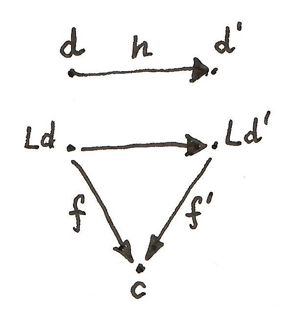
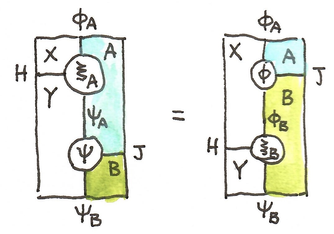
 , through which every arrow
  factorizes uniquely. That means, there is a unique arrow
  that makes the following triangle commute:
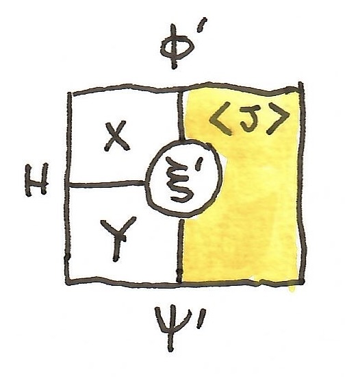
 , then we can easily construct the universal arrow as a pair
  , where
  is a component of the counit of the adjunction. Indeed, every
 .
.
 separately.
 , where
  is functor precomposition. Or as a string diagram:


 , where
  . Similarly, a graph of a relation is a set of pairs where
  is related to
  .
. . If the set is empty, it means that the objects are unrelated.
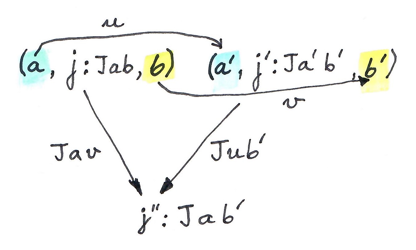
 , an object in the category of elements is a triple
  . We interpret
  as a witness that
  is a pair of morphisms
  such that:
 is the whiskering, or the lifting of a pair of morphisms, one of which is an identity, by the profunctor
  . We want the result, in both cases, to give us the same element of
  — the witness that
  .
.
 is a 0-cell
  equipped with two projections. Think of these projections as extracting the two objects from the triple that we used in the definition of a graph of a profunctor. Their relation to
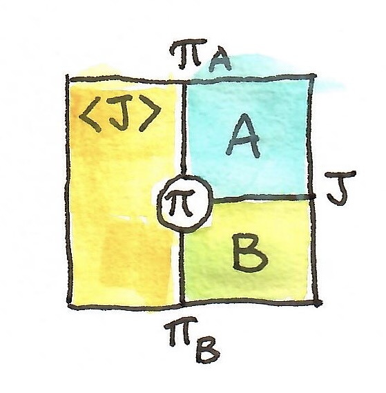

 is a natural transformation whose components are:
 and the result is an element of the set
  .
.  or
or  , both leading to the same result.
 . We postulate that for any 0-cell
  and
and  there is a unique factorization through the universal 2-cell
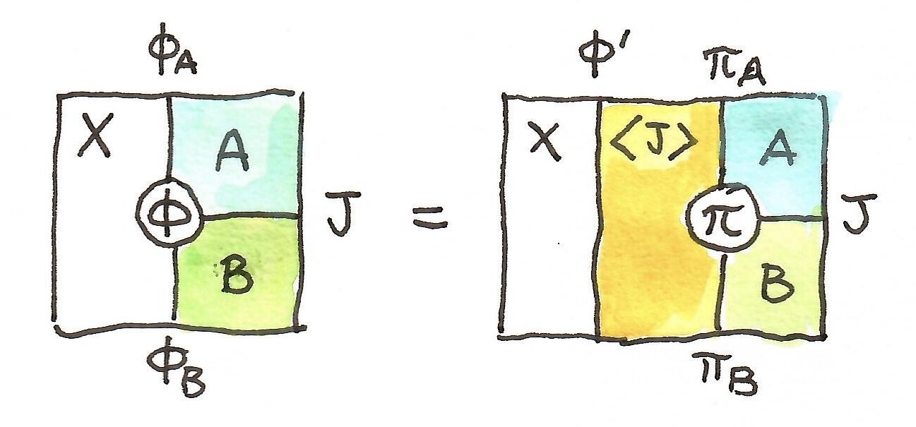


 , on objects, as:
 , as
, as  .
. . All we have to provide is two vertical arrows and a 2-cell. But to complete the picture, we should be able to construct a 2-cell from another horizontal 1-cell,
  together with a projection
  , such that:
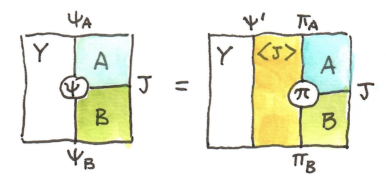


 :
:
 and
and  factor through it. Here’s the first factorization:

 , we get as the target a pair of morphisms:
 , we can construct such a pair as:
 this produces
  thus satisfying the 2-dimensional universal condition. The constraints on
  with
with  .
. that is somehow related to a vertical arrow
  . There are two 2-cells that illustrate this relation, but it’s not clear what their meaning is or how to use them.
 . Diagrammatically, we have:
 , is illustrated by the following diagrams:

 and
and  and turns them into
  and
and  . Then we shove the two counits below it (vertically postcompose), to bend the arrows
  and
and  .
.  and
and  , a cartesian square defines a horizontal arrow
  also called a restriction of

 . To this end we replace
  , together with two new vertical arrows
  and
and  that, just like
 over a pair of 1-cells
  , given the corresponding cartesian square
  .
.

 , with functors as morphisms.
 . In fact, profunctors can be considered arrows in the category
  . Not only that,
 is the identity profunctor with respect to this composition. It means that we have a way of talking about hom-sets and representables without peeking inside individual categories.
 with two (horizontal) profunctors
  and
and  .
. 
 is a function:

 is sometimes called the restriction of
  , in diagram order).
  is just an identity natural transformation:


 with the appropriate injection into the coend.
 implementing the functoriality of
 , is defined in

 stands for comPanion):
 .
.
 is the identity at


 :
:


 . Or we can consider a simpler case of the double category of sets and relations. We can also add more structure to the categories in question, for instance by considering monoidal categories; or even go meta, and study the double category of (weak) double categories
  .
. :
:
 for
for 
 and, consequently,
  is isomorphic to
  to be mapped to different “paths”
  , and we’d also like to have some non-trivial paths left over to play with.
 . In a cartesian category with weak equivalences, we can use an abstract definition of the object representing the space of all paths in
  is an object that factorizes the diagonal morphism
  , such that
  is a weak equivalence.

 , can be uniquely extended to all paths?
 to pick next. In fact, there might be only one value available to you — the “closest one” in the direction you’re going. To choose any other value, you’d have to “jump,” which would break continuity.
 by growing it from its initial value
  . You gradually extend it above the path
 .
. is a cofibration,
 . Such iterated types correspond to higher homotopies: paths between paths, and so on, ad infinitum. The structure that arises is called a weak infinity groupoid. It’s a category in which every morphism has an inverse (just follow the same path backwards), and category laws (identity or associativity) are satisifed up to higher morphisms (higher homotopies).
 is equal to
  . This is called definitional equality, since it’s just part of the definition. However, if we reverse the order of the addends and try to prove
  , there is no obvious shortcut. We have to prove it the hard way! This second type of equality is called propositional.
 written as
  , or even
  , if the type
 . Here,
  (type of equality of proofs of equality), and so on, ad infinitum. This used to be a bane of Martin Löf type theory, but it became a bounty for Homotopy Type Theory. So let’s imagine that the identity type may have non-trivial inhabitants. We’ll call these inhabitants paths. The trivial paths generated by
  to some type
  and
and  :
:

 , so it’s enough to specify how
 and
and  . Except that here we have a whole family of constructors

 . When projected down to
  , so we have:

 that maps
  . So, when projected back to


 . The section condition is:


 is a product of objects
  . The judgment:
 of type


 . The canonical example of a dependent type is a counted vector, which encodes length (a value of type
  ) in its type.
 . The type
  .
.

 may depend on
  ,
,  may depend on
  , and so on.

 , we have to make sure that
  is projected back to

 , a vector of lenght
 of the projection
  .
.