June 2026
Monthly Archive
June 30, 2026
Previously: Kan Extensions in Double Categories.
In programming, actegories play a central role in optics: lenses, prisms, traversals, etc. To understand actegories, let’s start with the definition of a monoidal category.
Monoidal Category
A monoidal category  is a category equipped with a tensor product. A tensor product is a functor
  . We assume that this product is associative and unital– up to isomorphism. It means that there is an invertible associator:

natural in all three arguments. We also have a unit object  and two (invertible, natural) unitors:


To get a better feel for it, we can try to model a monoidal category in Haskell. We parameterize it by the type of the tensor product, ten, which we want to be a Bifunctor:
The standard way to define a subcategory of Hask is to restrict the types of objects by imposing a constraint. Such a restriction has a special kind, Constraint:
A common example of such a constraint is a typeclass. For instance Monoid will restrict the objects of the category to be monoids. (In principle, we should also restrict the type of arrows, here to monoid morphisms.)
We can specify the unit of a monoidal category as an associated type (parameterized by ten):
type Unit ten :: Type
The unit should be an object of the category, so it should satisfy the constraint. We can encode this in our definition as a precondition: obj (Unit ten). This leads to a circularity, which we can overcome using the language pragma UndecidableSuperClasses:
Finally, we can add the associator and the unitors (and their inverses):
Notice the obj constraints in the type of these functions and the infix notation for the tensor.
Let’s work out a few examples. The simplest is the category of all types with a cartesian product as tensor.
We define Hask using an empty class, and we make all objects its instances:
Similarly, we can define a monoidal category with Either as the tensor product, or with Monoid as the object constraint.
Actegory
An actegory is a category that supports the action of a monoidal category. You may think of it as “multiplying” or “scaling” the objects of this category by objects of the monoidal category. The (left) action can be defined as a functor from the product category to  :
:

or, after currying, as a functor from to the endofunctor category:
![\triangleright \colon \mathbf M \to [C, C]](https://s0.wp.com/latex.php?latex=%5Ctriangleright+%5Ccolon+%5Cmathbf+M+%5Cto+%5BC%2C+C%5D&bg=ffffff&fg=29303b&s=0&c=20201002)
The coherency conditions are the invertible natural transformations that relate the action  to the tensor product
  and its unit :


The action is functorial in both arguments, so our Haskell translation pegs it, for simplicity, as a Bifunctor. (A Profunctor action is also possible. Categorically, it would correspond to using  as the monoidal category.)
Another simplifying assumption is that the action uniquely identifies the tensor product, encoded here as the functional dependency act -> ten.
The simplest example of an actegory is the self action of the cartesian product. Here, the monoidal category acts on itself:
Monoidal Functors
Actegories that use the same monoidal category for their actions form a category. The morphisms in this category are (strict) monoidal functors. These are functors that map one action to another:

In Haskell, we can model them as:
In fact, actegories form a bicategory, with action-preserving natural transformations acting between monoidal functors.
Here’s an interesting example of a monoidal functor between non-trivial actegories:
Haskell code is available here.
June 13, 2026
Previously: Kan extensions in Haskell.
In a double category that is also a proarrow equipment, we have the ability to bend arrows. In particular, in the definition of the counit of the right Kan extension:
we can bend the vertical  arrow, replacing it with its horizontal conjoint
  . In a profunctor equipment, this is just a representable profunctor
  .
.
A natural generalization is to replace this representable with a general profunctor. This way we get a definition of a right Kan extension along a profunctor  .
.
In a more general setting of a double category, the counit of the right Kan extension is a 2-cell:
The universal condition can be similarly generalized by bending the arrows.
However, the universal condition for pointwise right Kan extensions is stronger. It involves an additional horizontal 1-cell  . It states that any 2-cell
  of the shape below can be uniquely factorized through the counit
  :
:
Right Kan extensions in Haskell
In Haskell, the right Kan extension of a functor d along a profunctor j can be written as a data type:
This is a direct translation of the categorical formula that uses an end:

Compare this with the earlier implementation of the Kan extension, in which j was a functor:
The counit is a 2-cell from j to the identity profunctor (->):
The 2-cell Phi goes from the profunctor composition of j and h to the identity profunctor:
The factorization cell Phi' goes from h to identity:
For any Phi, we can find the corresponding Phi':
This function replaces the right adjoint used in the traditional definition of a Kan extension.
The result satisfies the factorization property:
Here vcomp is the vertical composition of 2-cells:
and funComp is hom-functor composition:
The computational meaning of the universal construction is that, in order to define a 2-cell (natural transformation) from some functor s to Ran j d along a profunctor h, it’s enough to provide a 2-cell from s to d along a composite Procompose j h.
Left Kan extensions
We can apply similar generalization to left Kan extensions. This time we start with the unit given by the 2-cell:
The universal condition that defines the pointwise left Kan extension of a vertical 1-cell  along a horizontal 1-cell is given by the following unique factorization:
Left Kan extensions in Haskell
In Haskell, we define the left Kan extension along a profunctor as an existential data type:
This is a direct translation of the coend formula:

The unit is a 2-cell:
The universal condition states that, for any 2-cell:
there is a unique 2-cell:
given by the mapping:
that uniquely factorizes through the unit eta:
Again, computationally, this defines a mapping-out property of the left Kan extension.
Complete Haskell code is available here: left Kan extensions, right Kan extensions.
June 8, 2026
Previously: Tabulation Tribulations.
If you think of functor composition as a form of multiplication, Kan extensions are an attempt to construct inverses of this multiplication. But unlike multiplication, composition is not symmetric, so we have extensions that attempt to undo precomposition, and lifts that do the same for postcomposition. Furthermore, there rarely is a single inverse to any form of composition, so we have the parsimonious right extensions and lifts, and the generous left extensions and lifts. We end up with four combinations that correspond to four different adjunctions:


We’ll concentrate on the extensions, since we can provide explicit point-wise formulas for them in cases that are of interest to us, that is in  and in
  .
.
Right Kan extensions
The definition of the right Kan extension relates the mapping out of the composition to the mapping into  . In Haskell, we can define them as two types:
The wavy arrows denote natural transformations:
To show that there is an adjunction we can either prove the (natural) isomorphism between Phi and Phi', or implement the unit and counit of the adjunction (together with zigzag identities):
In Haskell we can implement the right Kan extension as:
This is a straightforward translation of the categorical formula that uses an end:

The adjunction can then be implemented as a pair of mappings:
Or as the unit/counit pair:
Universal arrows
There is a third way, which gives a better starting point for generalizations. It can be used on an object-by-object basis, even if there is no global adjunction. It’s based on the idea of the universal arrow.
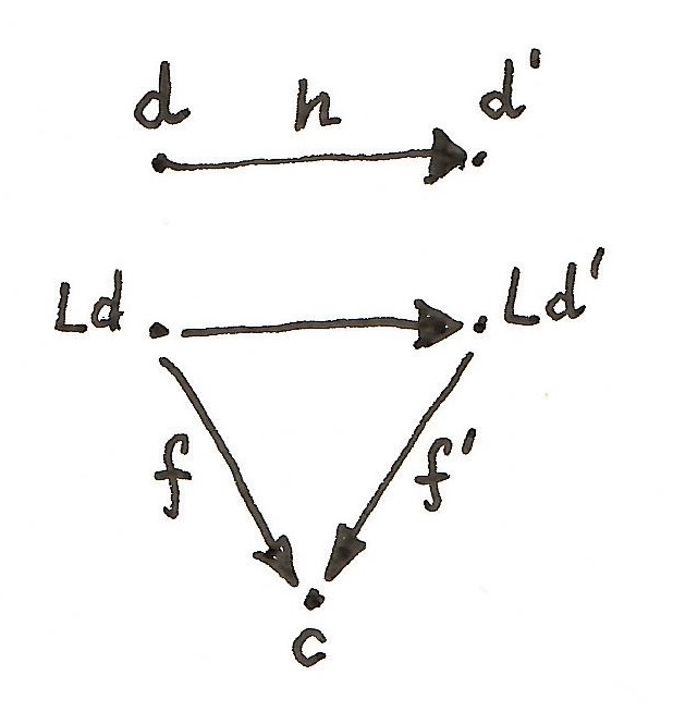
A universal arrow is a terminal object in the comma category. For a given functor  , the comma category
  consists of pairs
  . In other words, it’s a category of arrows from the image of
  to some fixed object
  . Morphisms in the comma category are arrows
  in
in  that make the corresponding triangles in commute:
A terminal object in is a pair  , through which every arrow
  factorizes uniquely. That means, there is a unique arrow
  that makes the following triangle commute:
If there is an adjunction  , then we can easily construct the universal arrow as a pair
  , where
  is a component of the counit of the adjunction. Indeed, every factorizes through :

where  .
.
The advantage of the universal arrow approach is that it’s pointwise. We can do it for each object  separately.
Reversing this process, rather than building an adjuncion, we can directly construct a universal arrow. We start by defining of a component of a counit. Then we postulate that any other counit-like mapping factorizes uniquely throught that counit.
Let’s see how it works for our definition of the right Kan extension. The counit has the following signature:
We can illustrate it with the following string diagram:
In general, the functors go between three different categories: A, B, and M. In Haskell we have just one category and three endofunctors.
Any other mapping of this form has the signature (replacing Ran j d with an arbitrary functor s):
Or, as a string diagram:
We postulate that, for every Phi, there is a unique Phi' that factorizes it through epsilon. That is, we have a function:
such that:
Modulo newtype shenanigans, this is exactly  , where
  is functor precomposition. Or as a string diagram:
Notice that rightAdj doesn’t appear anywhere in this construction.
The computational interpretation of this universal construction lets us calculate a mapping into a right Kan extension. Namely, to determine a natural transformation from some functor s to Ran j d, it’s enough to provide a mapping phi from Compose s j to d.
Left Kan extensions
We can now apply the same idea to the left Kan extension. This time we start with the unit:
We postulate that for any other mapping of this form (replacing Lan j d with and arbitrary s):
there is a unique Phi':
that factorizes it through eta:
In Haskell, the left Kan extension is given by the existential data type:
In category theory, this formula uses a coend:

Indeed, for any given Phi, we can obtain a Phi' by applying this function:
The result factorizes Phi through eta:
The computational interpretation of this universal construction let us calculate a mapping out of the left Kan extension.
See Haskell code for right and left Kan extensions.
Next, we’ll generalize these construction to a double category setting.