The fundamental premise of category theory is that it’s possible to fully capture the nature of objects by describing their interactions with other objects of the same type. Those interactions are encoded using morphisms: arrows between objects.
What about categories themselves? We define a category by describing its internals: objects and arrows. But true to the categorical credo, we should be able to capture the essence of a category by describing its interactions with other categories. (Small) categories are objects in the category of categories  , with functors as morphisms.
In fact has even more structure: functors between any two categories form a functor category, with natural transformations as morphisms. This makes a 2-category, with categories as 0-cells, functors as 1-cells, and natural transformations as 2-cells.
With this much structure, we can define a lot of categorical constructions. In particular, we can define adjunctions as pairs of functors equipped with the unit and counit natural transformations. We can also define monads as endofunctors equipped with the unit and multiplication natural transformations, and so on.
However, there are some categorical constructions that force us to look at the internals of categories. In particular, anything that involves representable functors cannot be defined without talking about hom-sets, which are internal to categories. In particular there are things like (weighted) limits or pointwise Kan extensions that rely on representability.
We somehow need to incorporate the information about hom-sets into the fabric of of the 2-category . At the minimum, we need to identify the hom-functors:

Such functors of mixed variance are called profunctors and, in general, they can go between different categories, as in  . In fact, profunctors can be considered arrows in the category
  . Not only that, is itself a bicategory, whose 0-cells are (small) categories, 1-cells are profunctors, and 2-cells are natural transformations between profunctors. Composition of profunctors is defined using the coend formula:

To be consistent with the Haskell implementation, I picked the arrow order, so you can read it  then
then  .
.
What is important is that the hom-functor  is the identity profunctor with respect to this composition. It means that we have a way of talking about hom-sets and representables without peeking inside individual categories.
The usual categorical laws, associativity and identity, are only satisfied up to isomorphism (that is up to invertible 2-cells), hence is called a bicategory and not a 2-category, whose laws are satisfied on the nose.
These two categories, the 2-category and the bicategory can be combined into a single double category, which we’ll call  . The 0-cells are the usual categories; but now we have two kinds of arrows: the vertical ones are functors, and the horizontal ones are profunctors. What glues them together are the 2-cells.
Here’s a 2-cell that combines two (vertical) functors  and
and  with two (horizontal) profunctors
  and
and  .
.
In our double category , this 2-cell is implemented as a natural transformation, whose component at the pair of objects  is a function:

It’s a member of the set of natural transformations, which can be written as an end:

The profunctor  is sometimes called the restriction of
  along
along  and
and  .
.
In an abstract double category, a 2-cell is just something that says that the particular four arrows in this configuration are related.
The same diagram can be transformed into a string diagram. Here, the 0-cells are the four areas, 1-cells form boundaries between those areas, and a 2-cell is a node connecting the four subdivisions:
We encode identity 1-cells in string diagrams by simply omitting the corresponding lines/arrows.
2-cells can be composed both horizontally and vertically by gluing them along identical edges.
In , horizontal composition of 2-cells corresponds to the (vertical) composition of natural transformations between profunctors (we’ll write this composition as a juxtaposition, as in  , in diagram order).
The identity 2-cell at a profunctor is just an identity natural transformation:
Vertical gluing of string diagrams results is a natural transformation between composite profunctors. For instance this diagram:
is a composition of two natural transformation:


whose component is a function:

By co-continuity of the coend, this is isomorphic to:

and is implemented by composing the product  with the appropriate injection into the coend.
The unit of vertical composition at a functor in is a 2-cell:
which is a natural transformation  implementing the functoriality of .
Companion and Conjoint
Given a functor we can construct two representable profunctors, the companion and the conjoint.
The companion is denoted by  or
or  . In , it is the profunctor generated by the following hom-functor:

A conjoint, which is denoted by  or
or  , is defined in as:

Notice that these two horizontal arrows go in opposite directions. The companion goes from  to
to  (the same as ), and the conjoint goes from to . Later we’ll see that they form an adjunction.
In these definitions we have used the hom-sets explicitly, something we were trying to avoid. We should therefore try to define the companions and the conjoints abstractly by listing their properties.
Companion
In a string diagram, the companion of a vertical arrow is represented by a left-pointing horizontal arrow:
It is equipped with two 2-cells called the unit and the counit (the subscript  stands for comPanion):
Indeed, using the rules for reading string diagrams in , the unit corresponds to a natural transformation:

which just expresses the functoriality of . The (invisible) horizontal line on the left stands for the identity profunctor  .
.
The counit in :

is trivially instantiated by the identity natural transformation.
There are two ways we can compose these two 2-cells. Both of them should result in some kind of identities. For instance, this is the horizontal composition:

where  is the identity at which, in is a functorial action of on the hom-set.
Similarly, vertical composition gives us:

Conjoint
The conjoint of is represented by the right-pointing horizontal arrow:
In , the conjoint is the representable profunctor: 
The conjoint is related to the original functor by its unit and counit 2-cells:
(here, the subscript  stands for conJoint). Their two compositions produce identity 2-cells:

Adjunction
We can also compose units with units and counits with counits by connecting the functor arrows:
These diagrams can be interpreted as the unit and counit of the adjunction  :
:


In , the profunctor composition is given by the coend, so we get, for the unit:

We use the Yoneda reduction to eliminate the coend:

The unit is then instantiated by the functoriality of .
The counit is:

By co-continuity of the coend, this is isomorphic to:

which is inhabited by the composition of hom-sets.
The Big Picture
We’ve seen how to combine the 2-category with the bicategory into one double category . In this double category every vertical arrow has a horizontal companion and every companion has a conjoint. A double category with this kind of structure is called a proarrow equipment. It has just enough structure to define abstractly such categorical constructions as weighted limits or pointwise Kan extensions. We can then apply those constructions to other double categories, without having to repeat ourselves.
One immediate application is to enriched categories and enriched profunctors, which form a proarrow equipment  . Or we can consider a simpler case of the double category of sets and relations. We can also add more structure to the categories in question, for instance by considering monoidal categories; or even go meta, and study the double category of (weak) double categories
  .
.






 -valued functors, so we immediately run into a problem when trying to describe them in a double category. And without presheaves, we can’t talk about the Yoneda lemma — the workhorse of category theory.
 of presheaves and a Yoneda vertical arrow (1-cell)
  — the Yoneda embedding. We take our guidance from the category of presheaves
 ![\hat A = [A, \mathbf{Set}]](https://s0.wp.com/latex.php?latex=%5Chat+A+%3D+%5BA%2C+%5Cmathbf%7BSet%7D%5D&bg=ffffff&fg=29303b&s=0&c=20201002) , where the Yoneda functor is defined as a representable functor:
, where the Yoneda functor is defined as a representable functor:
 and
and  . But it’s also possible to build a functor from a profunctor.
 .
. 

 ). I’ll use the notation
  for the category of presheaves on
 .)
.)
 is an object in the category
  ? We know what it means in
  , where:
![\hat A = [C^{op}, \mathbf{Set}]](https://s0.wp.com/latex.php?latex=%5Chat+A+%3D+%5BC%5E%7Bop%7D%2C+%5Cmathbf%7BSet%7D%5D&bg=ffffff&fg=29303b&s=0&c=20201002)


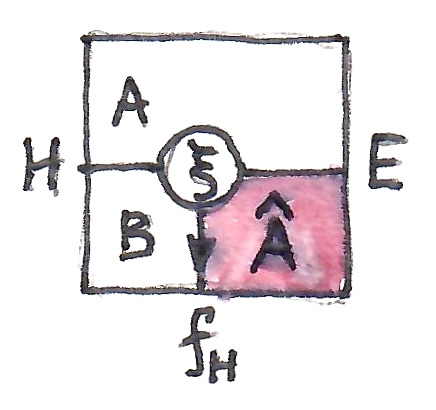
 is sometimes called the classifier for
  .
. . Its classifying arrow is the functor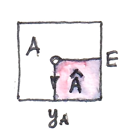


 arrow, we can redraw the original diagram defining the currying of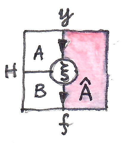


 an object (presheaf) in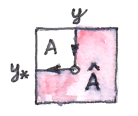
, \hat F)](https://s0.wp.com/latex.php?latex=%5Chat+F+a+%5Cto+%5BA%2C+%5Cmathbf%7BSet%7D%5D%28A%28-%2C+a%29%2C+%5Chat+F%29&bg=ffffff&fg=29303b&s=0&c=20201002)

 . The adjunction can be illustrated using the following 2-cells: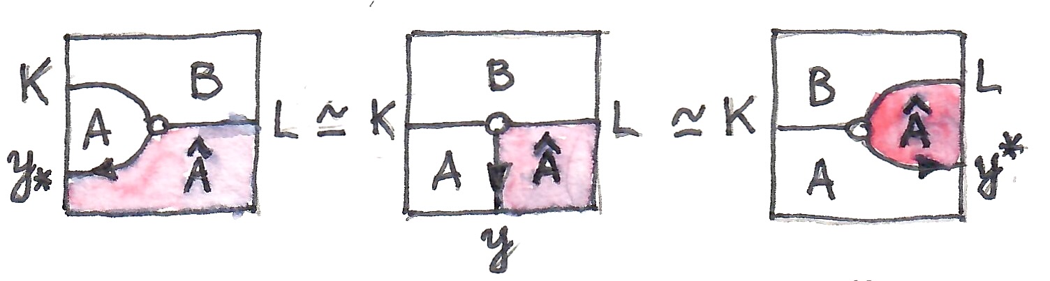
 and
and  arbitrary horizontal 1-cells.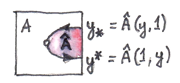


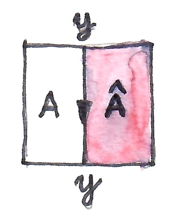
, A(-, a'))](https://s0.wp.com/latex.php?latex=A%28a%2C+a%27%29+%5Ccong+%5Chat+A+%28y+a%2C+y+a%27%29+%3D+%5BA%2C+%5Cmathbf%7BSet%7D%5D%28A%28-%2C+a%29%2C+A%28-%2C+a%27%29%29&bg=ffffff&fg=29303b&s=0&c=20201002)
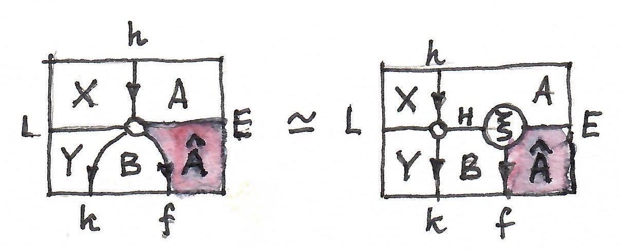
 such that for any horizontal 1-cell
  there exist a vertical 1-cell
  :
:
 :
:
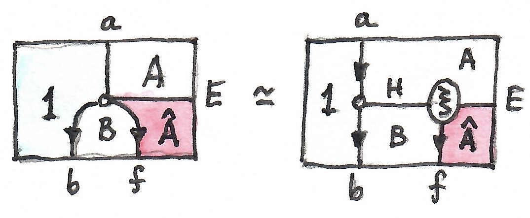
 and
and  with the terminal one-object/one-arrow category
  . A functor from such a category selects an object in the target category. Here, we pick two functors that select
  and
and  :
:
 . The right hand side is a horizontal composition of
  and
and  . The first one lets us fully reconstruct
  . Multiplication in this case means the action of a monoidal category
  . In other words, a Tambara module is a profunctor
  equipped with the transformation:
 , and dinatural in

 , where actegories are 0-cells, Tambara modules with coend composition are 1-cells, and natural transformations between them are 2-cells.
 . In Haskell this is:


 to
to  (it forgets the action). This functor has a left adjoint. For any profunctor
 . Indeed, applying the Yoneda reduction, we get:
![\mathbf M \to [C, C]](https://s0.wp.com/latex.php?latex=%5Cmathbf+M+%5Cto+%5BC%2C+C%5D&bg=ffffff&fg=29303b&s=0&c=20201002) , can be internalized in
, can be internalized in  if it has a right adjoint:


![\int^{c \colon [\mathbb N , Set]} C(s, \sum_n c_n \times a^n) \times C (\sum_m c_m \times b^m, t)](https://s0.wp.com/latex.php?latex=%5Cint%5E%7Bc+%5Ccolon+%5B%5Cmathbb+N+%2C+Set%5D%7D+C%28s%2C+%5Csum_n+c_n+%5Ctimes+a%5En%29+%5Ctimes+C+%28%5Csum_m+c_m+%5Ctimes+b%5Em%2C+t%29&bg=ffffff&fg=29303b&s=0&c=20201002)
 is a natural-number-indexed family of objects with a monoidal structure given by convolution; and
  and
and  are powers.

 is automatically a monoid in


 , is illustrated by the following diagrams:

 and
and  and turns them into
  and
and  . Then we shove the two counits below it (vertically postcompose), to bend the arrows
  and
and  .
.  also called a restriction of
 . To this end we replace
  , together with two new vertical arrows
  and
and  that, just like
  (see the left diagram below).
 from
from  over a pair of 1-cells
  , given the corresponding cartesian square
  .
.


