You might have heard people say that functional programming is more academic, and real engineering is done in imperative style. I’m going to show you that real engineering is functional, and I’m going to illustrate it using a computer game that is designed by engineers for engineers. It’s a simulation game called Factorio, in which you are given resources that you have to explore, build factories that process them, create more and more complex systems, until you are finally able to launch a spaceship that may take you away from an inhospitable planet. If this is not engineering at its purest then I don’t know what is. And yet almost all you do when playing this game has its functional programming counterparts and it can be used to teach basic concepts of not only programming but also, to some extent, category theory. So, without further ado, let’s jump in.
Functions
The building blocks of every programming language are functions. A function takes input and produces output. In Factorio they are called assembling machines, or assemblers. Here’s an assembler that produces copper wire.

If you bring up the info about the assembler you’ll see the recipe that it’s using. This one takes one copper plate and produces a pair of coils of copper wire.

This recipe is really a function signature in a strongly typed system. We see two types: copper plate and copper wire, and an arrow between them. Also, for every copper plate the assembler produces a pair of copper wires. In Haskell we would declare this function as
makeCopperWire :: CopperPlate -> (CopperWire, CopperWire)
Not only do we have types for different components, but we can combine types into tuples–here it’s a homogenous pair (CopperWire, CopperWire). If you’re not familiar with Haskell notation, here’s what it might look like in C++:
std::pair<CopperWire, CopperWire> makeCopperWire(CopperPlate);
Here’s another function signature in the form of an assembler recipe:

It takes a pair of iron plates and produces an iron gear wheel. We could write it as
makeGear :: (IronPlate, IronPlate) -> Gear
or, in C++,
Gear makeGear(IronPlate, IronPlate);
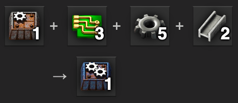
Many recipes require a combination of differently typed ingredients, like the one for producing red science packs

We would declare this function as:
makeRedScience :: (CopperPlate, Gear) -> RedScience
Pairs are examples of product types. Factorio recipes use the plus sign to denote tuples; I guess this is because we often read a sum as “this and this”, and “and” introduces a product type. The assembler requires both inputs to produce the output, so it accepts a product type. If it required either one, we’d call it a sum type.
We can also tuple more than two ingredients, as in this recipe for producing electronic circuits (or green circuits, as they are commonly called)

makeGreenCircuit ::
  (CopperWire, CopperWire, CopperWire, IronPlate) -> GreenCircuit
Now suppose that you have at your disposal the raw ingeredients: iron plates and copper plates. How would you go about producing red science or green circuits? This is where function composition kicks in. You can pass the output of the copper wire assembler as the input to the green circuit assembler. (You will still have to tuple it with an iron plate.)
Similarly, you can compose the gear assembler with the red science assembler.
The result is a new function with the following signature
makeRedScienceFrom ::
    (CopperPlate, IronPlate, IronPlate) -> RedScience
And this is the implementation:
makeRedScienceFrom (cu, fe1, fe2) =
    makeRedScience (cu, makeGear (fe1, fe2))
You start with one copper plate and two iron plates. You feed the iron plates to the gear assembler. You pair the resulting gear with the copper plate and pass it to the red science assembler.
Most assemblers in Factorio take more than one argument, so I couldn’t come up with a simpler example of composition, one that wouldn’t require untupling and retupling. In Haskell we usually use functions in their curried form (we’ll come back to this later), so composition is easy there.
Composition is also a feature of a category, so we should ask the question if we can treat assemblers as arrows in a category. Their composition is obviously associative. But do we have an equivalent of an identity arrow? It is something that takes input of some type and returns it back unchanged. And indeed we have things called inserters that do exactly that. Here’s an inserter between two assemblers.

In fact, in Factorio, you have to use an inserter for direct composition of assemblers, but that’s an implementation detail (technically, inserting an identity function doesn’t change anything).
An inserter is actually a polymorphic function, just like the identity function in Haskell
inserter :: a -> a
inserter x = x
It works for any type a.
But the Factorio category has more structure. As we have seen, it supports finite products (tuples) of arbitrary types. Such a category is called cartesian. (We’ll talk about the unit of this product later.)
Notice that we have identified multiple Factorio subsystem as functions: assemblers, inserters, compositions of assemblers, etc. In a programming language they would all be just functions. If we were to design a language based on Factorio (we could call it Functorio), we would enclose the composition of assemblers into an assembler, or even make an assembler that takes two assemblers and produces their composition. That would be a higher-order assembler.
Higher order functions
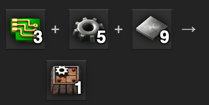
The defining feature of functional languages is the ability to make functions first-class objects. That means the ability to pass a function as an argument to another function, and to return a function as a result of another function. For instance, we should have a recipe for producing assemblers. And, indeed, there is such recipe. All it needs is green circuits, some gear wheels, and a few iron plates:

If Factorio were a strongly typed language all the way, there would be separate recipes for producing different assemblers (that is assemblers with different recipes). For instance, we could have:
makeRedScienceAssembler ::
   (GreenCircuit, Gear, IronPlate) -> RedScienceAssembler
Instead, the recipe produces a generic assembler, and it lets the player manually set the recipe in it. In a way, the player provides one last ingredient, an element of the enumeration of all possible recipes. This enumeration is displayed as a menu of choices:

After all, Factorio is an interactive game.
Since we have identified the inserter as the identity function, we should have a recipe for producing it as well. And indeed there is one:

Do we also have functions that take functions as arguments? In other words, recipes that use assemblers as input? Indeed we do:

Again, this recipe accepts a generic assembler that hasn’t been assigned its own recipe yet.
This shows that Factorio supports higher-order functions and is indeed a functional language. What we have here is a way of treating functions (assemblers) not only as arrows between objects, but also as objects that can be produced and consumed by functions. In category theory, such objectified arrow types are called exponential objects. A category in which arrow types are represented as objects is called closed, so we can view Factorio as a cartesian closed category.
In a strongly typed Factorio, we could say that the object RedScienceAssembler

is equivalent to its recipe
type RedScienceAssembler =
    (CopperPlate, Gear) -> RedScience
We could then write a higher-order recipe that produces this particular assembler as:
makeRedScienceAssembler ::
     (GreenCircuit, Gear, IronPlate)
  -> ((CopperPlate, Gear) -> RedScience)
Similarly, in a strongly typed Factorio we would replace this higher-order recipe

with the following signature
makeGreenScience :: ((a -> a), Belt) -> GreenScience
assuming that the inserter is a polymorphic function a -> a.
Linear types
There is one important aspect of functional programming that seems to be broken in Factorio. Functions are supposed to be pure: mutation is a no-no. And in Factorio we keep talking about assemblers consuming resources. A pure function doesn’t consume its arguments–you may pass the same item to many functions and it will still be there. Dealing with resources is a real problem in programming in general, including purely functional languages. Fortunately there are clever ways of dealing with it. In C++, for instance, we can use unique pointers and move semantics, in Rust we have ownership types, and Haskell recently introduced linear types. What Factorio does is very similar to Haskell’s linear types. A linear function is a function that is guaranteed to consume its argument. Functorio assemblers are linear functions.
Factorio is all about consuming and transforming resources. The resources originate as various ores and coal in mines. There are also trees that can be chopped to yield wood, and liquids like water or crude oil. These external resources are then consumed, linearly, by your industry. In Haskell, we would implement it by passing a linear function called a continuation to the resource producer. A linear function guarantees to consume the resource completely (no resource leaks) and not to make multiple copies of the same resource. These are the guarantees that the Factorio industrial complex provides automatically.
Currying
Of course Factorio was not designed to be a programming language, so we can’t expect it to implement every aspect of programming. It is fun though to imagine how we would translate some more advanced programming features into Factorio. For instance, how would currying work? To support currying we would first need partial application. The idea is pretty simple. We have already seen that assemblers can be treated as first class objects. Now imagine that you could produce assemblers with a set recipe (strongly typed assemblers). For instance this one:
It’s a two-input assembler. Now give it a single copper plate, which in programmer speak is called partial application. It’s partial because we haven’t supplied it with an iron gear. We can think of the result of partial application as a new single-input assembler that expects an iron gear and is able to produce one beaker of red science. By partially applying the function makeRedScience
makeRedScience :: (CopperPlate, Gear) -> RedScience
we have created a new function of the type
Gear -> RedScience
In fact we have just designed a process that gave us a (higher-order) function that takes a copper plate and creates a “primed” assembler that only needs an iron gear to produce red science:
makeGearToRedScience :: CopperPlate -> (Gear -> RedScience)
In Haskell, we would implement this function using a lambda expression
makeGearToRedScience cu = \gear -> makeRedScience (cu, gear)
Now we would like to automate this process. We want to have something that takes a two-input assembler, for instance makeRedScience, and returns a single input assembler that produces another “primed” single-input assembler. The type signature of this beast would be:
curryRedScienceAssembler ::
     ((CopperPlate, Gear) -> RedScience)  -- RedScienceAssembler
  -> (CopperPlate -> (Gear -> RedScience))
We would implement it as a double lambda:
curryRedScienceAssembler rsAssembler =
  \cu -> (\gear -> rsAssembler (cu, gear))
Notice that it really doesn’t matter what the concrete types are. What’s important is that we can turn a function that takes a pair of arguments into a function that returns a function. We can make it fully polymorphic:
curry :: ((a, b) -> c)
       -> (a -> (b -> c))
Here, the type variables a, b and c can be replaced with any types (in particular, CopperPlate, Gear, and RedScience).
This is a Haskell implementation:
curry f = \a -> \b -> f (a, b)
Functors
So far we haven’t talked about how arguments (items) are delivered to functions (assemblers). We can manually drop items into assemblers, but that very quickly becomes boring. We need to automate the delivery systems. One way of doing it is by using some kind of containers: chests, train wagons, barrels, or conveyor belts. In programming we call these functors. Strictly speaking a functor can hold only one type of items at a time, so a chest of iron plates should be a different type than a chest of gears. Factorio doesn’t enforce this but, in practice, we rarely mix different types of items in one container.
The important property of a functor is that you can apply a function to its contents. This is best illustrated with conveyor belts. Here we take the recipe that turns a copper plate into copper wire and apply it to a whole conveyor belt of copper (coming from the right) to produce a conveyor belt of copper wire (going to the left).

The fact that a belt can carry any type of items can be expressed as a type constructor–a data type parameterized by an arbitrary type a
data Belt a
You can apply it to any type to get a belt of specific items, as in
Belt CopperPlate
We will model belts as Haskell lists.
data Belt a = MakeBelt [a]
The fact that it’s a functor is expressed by implementing a polymorphic function mapBelt
mapBelt :: (a -> b) -> (Belt a -> Belt b)
This function takes a function a->b and produces a function that transforms a belt of as to a belt of bs. So to create a belt of (pairs of) copper wire we’ll map the assembler that implements makeCoperWire over a belt of CopperPlate
makeBeltOfWire :: (Belt CopperPlate) -> (Belt (CopperWire, CopperWire))
makeBeltOfWire = mapBelt makeCopperWire
You may think of a belt as corresponding to a list of elements, or an infinite stream, depending on the way you use it.
In general, a type constructor F is called a functor if it supports the mapping of a function over its contents:
map :: (a -> b) -> (F a -> F b)
Sum types
Uranium ore processing is interesting. It is done in a centrifuge, which accepts uranium ore and produces two isotopes of Uranium.

The new thing here is that the output is probabilistic. Most of the time (on average, 99.3% of the time) you’ll get Uranium 238, and only occasionally (0.7% of the time) Uranium 235 (the glowy one). Here the plus sign is used to actually encode a sum type. In Haskell we would use the Either type constructor, which generates a sum type:
makeUranium :: UraniumOre -> Either U235 U238
In other languages you might see it called a tagged union.
The two alternatives in the output type of the centrifuge require different actions: U235 can be turned into fuel cells, whereas U238 requires reprocessing. In Haskell, we would do it by pattern matching. We would apply one function to deal with U235 and another to deal with U238. In Factorio this is accomplished using filter inserters (a.k.a., purple inserters). A filter inserter corresponds to a function that picks one of the alternatives, for instance:
filterInserterU235 :: Either U235 U238 -> Maybe U235
The Maybe data type (or Optional in some languages) is used to accommodate the possibility of failure: you can’t get U235 if the union contained U238.
Each filter inserter is programmed for a particular type. Below you see two purple inserters used to split the output of the centrifuge into two different chests:

Incidentally, a mixed conveyor belt may be seen as carrying a sum type. The items on the belt may be, for instance, either copper wire or steel plates, which can be written as Either CopperWire SteelPlate. You don’t even need to use purple inserters to separate them, as any inserter becomes selective when connected to the input of an assembler. It will only pick up the items that are the inputs of the recipe for the given assembler.
Monoidal functors
Every conveyor belt has two sides, so it’s natural to use it to transport pairs. In particular, it’s possible to merge a pair of belts into one belt of pairs.

We don’t use an assembler to do it, just some belt mechanics, but we can still think of it as a function. In this case, we would write it as
(Belt CopperPlate, Belt Gear) -> Belt (CopperPlate, Gear)
In the example above, we map the red science function over it
streamRedScience :: Belt (CopperPlate, Gear) -> Belt RedScience
streamRedScience beltOfPairs = mapBelt makeRedScience beltOfPairs
Since makeRedScience has the signature
makeRedScience :: (CopperPlate, Gear) -> RedScience
it all type checks.
Since we can apply belt merging to any type, we can write it as a polymorphic function
mergeBelts :: (Belt a, Belt b) -> Belt (a, b)
mergeBelts (MakeBelt as, MakeBelt bs) = MakeBelt (zip as bs)
(In our Haskell model, we have to zip two lists together to get a list of pairs.)
Belt is a functor. In general, a functor that has this kind of merging ability is called a monoidal functor, because it preserves the monoidal structure of the category. Here, the monoidal structure of the Factorio category is given by the product (pairing). Any monoidal functor F must preserve the product:
(F a, F b) -> F (a, b)
There is one more aspect to monoidal structure: the unit. The unit, when paired with anything, does nothing to it. More precisely, a pair (Unit, a) is, for all intents and purposes, equivalent to a. The best way to understand the unit in Factorio is to ask the question: The belt of what, when merged with the belt of a, will produce a belt of a? The answer is: the belt of nothing. Merging an empty belt with any other belt, makes no difference.

So emptiness is the monoidal unit, and we have, for instance:
(Belt CopperPlate, Belt Nothing) -> Belt CopperPlate
The ability to merge two belts, together with the ability to create an empty belt, makes Belt a monoidal functor. In general, besides preserving the product, the condition for the functor F to be monoidal is the ability to produce
F Nothing
Most functors, at least in Factorio, are not monoidal. For instance, chests cannot store pairs.
Applicative functors
As I mentioned before, most assembler recipes take multiple arguments, which we modeled as tuples (products). We also talked about partial application which, essentially, takes an assembler and one of the ingredients and produces a “primed” assembler whose recipe requires one less ingredient. Now imagine that you have a whole belt of a single ingredient, and you map an assembler over it. In current Factorio, this assembler will accept one item and then get stuck waiting for the rest. But in our extended version of Factorio, which we call Functorio, mapping a multi-input assembler over a belt of single ingredient should produce a belt of “primed” assemblers. For instance, the red science assembler has the signature
(CopperPlate, Gear) -> RedScience
When mapped over a belt of CopperPlate it should produce a belt of partially applied assemblers, each with the recipe:
Gear -> RedScience
Now suppose that you have a belt of gears ready. You should be able to produce a belt of red science. If there only were a way to apply the first belt over the second belt. Something like this:
(Belt (Gear -> RedScience), Belt Gear) -> Belt RedScience
Here we have a belt of primed assemblers and a belt of gears and the output is a belt of red science.
A functor that supports this kind of merging is called an applicative functor. Belt is an applicative functor. In fact, we can tell that it’s applicative because we’ve established that it’s monoidal. Indeed, monoidality lets us merge the two belts to get a belt of pairs
Belt (Gear -> RedScience, Gear)
We know that there is a way of applying the Gear->RedScience assembler to a Gear resulting in RedScience. That’s just how assemblers work. But for the purpose of this argument, let’s give this application an explicit name: eval.
eval :: (Gear -> RedScience, Gear) -> RedScience
eval (gtor, gr) = gtor gr
(gtor gr is just Haskell syntax for applying the function gtor to the argument gr). We are abstracting the basic property of an assembler that it can be applied to an item.
Now, since Belt is a functor, we can map eval over our belt of pairs and get a belt of RedScience.
apBelt :: (Belt (Gear -> RedScience), Belt Gear) -> Belt RedScience
apBelt (gtors, gear) = mapBelt eval (mergeBelts (gtors, gears))
Going back to our original problem: given a belt of copper plate and a belt of gear, this is how we produce a belt of red science:
redScienceFromBelts :: (Belt CopperPlate, Belt Gear) -> Belt RedScience
redScienceFromBelts (beltCu, beltGear) =
  apBelt (mapBelt (curry makeRedScience) beltCu, beltGear)
We curry the two-argument function makeRedScience and map it over the belt of copper plates. We get a beltful of primed assemblers. We then use apBelt to apply these assemblers to a belt of gears.
To get a general definition of an applicative functor, it’s enough to replace Belt with generic functor F, CopperPlate with a, and Gear with b. A functor F is applicative if there is a polymorphic function:
(F (a -> b), F a) -> F b
or, in curried form,
F (a -> b) -> F a -> F b
To complete the picture, we also need the equivalent of the monoidal unit law. A function called pure plays this role:
pure :: a -> F a
This just tell you that there is a way to create a belt with a single item on it.
Monads
In Factorio, the nesting of functors is drastically limited. It’s possible to produce belts, and you can put them on belts, so you can have a beltful of belts, Belt Belt. Similarly you can store chests inside chests. But you can’t have belts of loaded belts. You can’t pick a belt filled with copper plates and put it on another belt. In other words, you cannot transport beltfuls of stuff. Realistically, that wouldn’t make much sense in real world, but in Functorio, this is exactly what we need to implement monads. So imagine that you have a belt carrying a bunch of belts that are carrying copper plates. If belts were monadic, you could turn this whole thing into a single belt of copper plates. This functionality is called join (in some languages, “flatten”):
join :: Belt (Belt CopperPlate) -> Belt CopperPlate
This function just gathers all the copper plates from all the belts and puts them on a single belt. You can thing of it as concatenating all the subbelts into one.
Similarly, if chests were monadic (and there’s no reason they shouldn’t be) we would have:
join :: Chest (Chest Gear) -> Chest Gear
A monad must also support the applicative pure (in Haskell it’s called return) and, in fact, every monad is automatically applicative.
Conclusion
There are many other aspects of Factorio that lead to interesting topics in programming. For instance, the train system requires dealing with concurrency. If two trains try to enter the same crossing, we’ll have a data race which, in Functorio, is called a train crash. In programming, we avoid data races using locks. In Factorio, they are called train signals. And, of course, locks lead to deadlocks, which are very hard to debug in Factorio.
In functional programming we might use STM (Software Transactional Memory) to deal with concurrency. A train approaching a crossing would start a crossing transaction. It would temporarily ignore all other trains and happily make the crossing. Then it would attempt to commit the crossing. The system would then check if, in the meanwhile, another train has successfully commited the same crossing. If so, it would say “oops! try again!”.


![\cong \int^{\langle C, p \rangle : \mathcal{C}/B} (\mathcal{C}/B)( S, C \times_B A) \times (\mathcal{C}/B)(C , [A', S']_B)](https://s0.wp.com/latex.php?latex=%5Ccong+%5Cint%5E%7B%5Clangle+C%2C+p+%5Crangle+%3A+%5Cmathcal%7BC%7D%2FB%7D+%28%5Cmathcal%7BC%7D%2FB%29%28+S%2C+C+%5Ctimes_B+A%29+%5Ctimes+%28%5Cmathcal%7BC%7D%2FB%29%28C+%2C+%5BA%27%2C+S%27%5D_B%29+&bg=ffffff&fg=29303b&s=0&c=20201002)
![(\mathcal{C}/B)( S, [A', S']_B \times_B A)](https://s0.wp.com/latex.php?latex=%28%5Cmathcal%7BC%7D%2FB%29%28+S%2C+%5BA%27%2C+S%27%5D_B+%5Ctimes_B+A%29+&bg=ffffff&fg=29303b&s=0&c=20201002)
![[A', S']_B](https://s0.wp.com/latex.php?latex=%5BA%27%2C+S%27%5D_B&bg=ffffff&fg=29303b&s=0&c=20201002)
![\left [\left \langle A' \atop p \right \rangle, \left \langle S' \atop q \right \rangle \right ] \cong \Pi_p \left(p^* \left \langle S' \atop q \right \rangle \right)](https://s0.wp.com/latex.php?latex=%5Cleft+%5B%5Cleft+%5Clangle+A%27+%5Catop+p+%5Cright+%5Crangle%2C+%5Cleft+%5Clangle+S%27+%5Catop+q+%5Cright+%5Crangle+%5Cright+%5D+%5Ccong+%5CPi_p+%5Cleft%28p%5E%2A+%5Cleft+%5Clangle+S%27+%5Catop+q+%5Cright+%5Crangle+%5Cright%29&bg=ffffff&fg=29303b&s=0&c=20201002)


![(\mathbf{Set}/\mathbb{N})\left(\left \langle {C \atop p} \right \rangle, \left[ \left \langle {L(b) \atop \mathit{len}} \right \rangle, \left \langle {\mathbb{N} \times t \atop \pi_1} \right \rangle \right] \right)](https://s0.wp.com/latex.php?latex=%28%5Cmathbf%7BSet%7D%2F%5Cmathbb%7BN%7D%29%5Cleft%28%5Cleft+%5Clangle+%7BC+%5Catop+p%7D+%5Cright+%5Crangle%2C+%5Cleft%5B+%5Cleft+%5Clangle+%7BL%28b%29+%5Catop+%5Cmathit%7Blen%7D%7D+%5Cright+%5Crangle%2C+%5Cleft+%5Clangle+%7B%5Cmathbb%7BN%7D+%5Ctimes+t+%5Catop+%5Cpi_1%7D+%5Cright+%5Crangle+%5Cright%5D+%5Cright%29+&bg=ffffff&fg=29303b&s=0&c=20201002)

![O(a, b; s, t) \cong \mathbf{Set} \left( s, U\left( \left[ \left \langle {L(b) \atop \mathit{len}} \right \rangle, \left \langle {\mathbb{N} \times t \atop \pi_1} \right \rangle \right] \times \left \langle {L(a) \atop \mathit{len}} \right \rangle \right) \right)](https://s0.wp.com/latex.php?latex=O%28a%2C+b%3B+s%2C+t%29+%5Ccong+%5Cmathbf%7BSet%7D+%5Cleft%28+s%2C+U%5Cleft%28+%5Cleft%5B+%5Cleft+%5Clangle+%7BL%28b%29+%5Catop+%5Cmathit%7Blen%7D%7D+%5Cright+%5Crangle%2C+%5Cleft+%5Clangle+%7B%5Cmathbb%7BN%7D+%5Ctimes+t+%5Catop+%5Cpi_1%7D+%5Cright+%5Crangle+%5Cright%5D+%5Ctimes+%5Cleft+%5Clangle+%7BL%28a%29+%5Catop+%5Cmathit%7Blen%7D%7D+%5Cright+%5Crangle+%5Cright%29+%5Cright%29+&bg=ffffff&fg=29303b&s=0&c=20201002)

 leaves: a traversal would return a list of leaves, and it would allow you to replace them with a new list. The problem is that the size of the list you pass to the setter cannot be arbitrary—it must match the number of leaves in the particular tree. This is why, in Haskell, the setter and the getter are usually combined in a single function:


 . (The sum is really a coend over
 ![\int^{c \colon [\mathbb{N}, \mathbf{Set}]} \mathbf{Set}\big(s, \sum_n c_n \times a^n\big) \times \mathbf{Set}\big( \sum_m c_m \times b^m, t\big)](https://s0.wp.com/latex.php?latex=%5Cint%5E%7Bc+%5Ccolon+%5B%5Cmathbb%7BN%7D%2C+%5Cmathbf%7BSet%7D%5D%7D+%5Cmathbf%7BSet%7D%5Cbig%28s%2C+%5Csum_n+c_n+%5Ctimes+a%5En%5Cbig%29+%5Ctimes+%5Cmathbf%7BSet%7D%5Cbig%28+%5Csum_m+c_m+%5Ctimes+b%5Em%2C+t%5Cbig%29+&bg=ffffff&fg=29303b&s=0&c=20201002)
![\int^{c \colon [\mathbb{N}, \mathbf{Set}]} \mathbf{Set}\big(s, \sum_n c_n \times a^n\big) \times \prod_m \mathbf{Set}\big( c_m \times b^m, t\big)](https://s0.wp.com/latex.php?latex=%5Cint%5E%7Bc+%5Ccolon+%5B%5Cmathbb%7BN%7D%2C+%5Cmathbf%7BSet%7D%5D%7D+%5Cmathbf%7BSet%7D%5Cbig%28s%2C+%5Csum_n+c_n+%5Ctimes+a%5En%5Cbig%29+%5Ctimes+%5Cprod_m+%5Cmathbf%7BSet%7D%5Cbig%28+c_m+%5Ctimes+b%5Em%2C+t%5Cbig%29+&bg=ffffff&fg=29303b&s=0&c=20201002)
![\int^{c \colon [\mathbb{N}, \mathbf{Set}]} \mathbf{Set}\big(s, \sum_n c_n \times a^n\big) \times \prod_m \mathbf{Set}\big( c_m, \mathbf{Set}( b^m, t)\big)](https://s0.wp.com/latex.php?latex=%5Cint%5E%7Bc+%5Ccolon+%5B%5Cmathbb%7BN%7D%2C+%5Cmathbf%7BSet%7D%5D%7D+%5Cmathbf%7BSet%7D%5Cbig%28s%2C+%5Csum_n+c_n+%5Ctimes+a%5En%5Cbig%29+%5Ctimes+%5Cprod_m+%5Cmathbf%7BSet%7D%5Cbig%28+c_m%2C+%5Cmathbf%7BSet%7D%28+b%5Em%2C+t%29%5Cbig%29+&bg=ffffff&fg=29303b&s=0&c=20201002)
![[\mathbb{N}, \mathbf{Set}]](https://s0.wp.com/latex.php?latex=%5B%5Cmathbb%7BN%7D%2C+%5Cmathbf%7BSet%7D%5D&bg=ffffff&fg=29303b&s=0&c=20201002)
![\int^{c \colon [\mathbb{N}, \mathbf{Set}]} \mathbf{Set}\big(s, \sum_n c_n \times a^n\big) \times [\mathbb{N}, \mathbf{Set}]\big( c_-, \mathbf{Set}( b^-, t)\big)](https://s0.wp.com/latex.php?latex=%5Cint%5E%7Bc+%5Ccolon+%5B%5Cmathbb%7BN%7D%2C+%5Cmathbf%7BSet%7D%5D%7D+%5Cmathbf%7BSet%7D%5Cbig%28s%2C+%5Csum_n+c_n+%5Ctimes+a%5En%5Cbig%29+%5Ctimes+%5B%5Cmathbb%7BN%7D%2C+%5Cmathbf%7BSet%7D%5D%5Cbig%28+c_-%2C+%5Cmathbf%7BSet%7D%28+b%5E-%2C+t%29%5Cbig%29+&bg=ffffff&fg=29303b&s=0&c=20201002)
 to get:

![F \colon \mathcal{M} \to [\mathcal{C}, \mathcal{C}]](https://s0.wp.com/latex.php?latex=F+%5Ccolon+%5Cmathcal%7BM%7D+%5Cto+%5B%5Cmathcal%7BC%7D%2C+%5Cmathcal%7BC%7D%5D+&bg=ffffff&fg=29303b&s=0&c=20201002)
![G \colon \mathcal{M} \to [\mathcal{D}, \mathcal{D}]](https://s0.wp.com/latex.php?latex=G+%5Ccolon+%5Cmathcal%7BM%7D+%5Cto+%5B%5Cmathcal%7BD%7D%2C+%5Cmathcal%7BD%7D%5D+&bg=ffffff&fg=29303b&s=0&c=20201002)

 ,
,  is from


 into
into  . In physics, we would say that the paths are “invariant” under the transformation, but in category theory we are fine with a one-way mapping.
 to
to  .
. , such a mapping exists, then these states are related. There exists a transformation and a pair of morphisms that are secretly used in the path integral to extend the original path.
 to
to  by first applying
  and then lifting the two morphisms. The converse is also true: if every path can be extended then such a pair of morphisms must exist.
 can be interpreted both as parameterizing a monoidal action and the residue left over after removing the focus.
 acting as the unit with respect to taking the end. It takes an
  and returns an
  that we’ve encountered before. They are parameterized by objects in

![\int_{x} \mathbf{Set}\big(\mathcal{C}(a, x), fx\big) = [\mathcal{C}, \mathbf{Set}]\big(\mathcal{C}(a, -), f\big)](https://s0.wp.com/latex.php?latex=%5Cint_%7Bx%7D+%5Cmathbf%7BSet%7D%5Cbig%28%5Cmathcal%7BC%7D%28a%2C+x%29%2C+fx%5Cbig%29+%3D+%5B%5Cmathcal%7BC%7D%2C+%5Cmathbf%7BSet%7D%5D%5Cbig%28%5Cmathcal%7BC%7D%28a%2C+-%29%2C+f%5Cbig%29&bg=ffffff&fg=29303b&s=0&c=20201002)
![[\mathcal{C}, \mathbf{Set}]\big(\mathcal{C}(s, -), \mathcal{C}(a, -) \big)](https://s0.wp.com/latex.php?latex=%5B%5Cmathcal%7BC%7D%2C+%5Cmathbf%7BSet%7D%5D%5Cbig%28%5Cmathcal%7BC%7D%28s%2C+-%29%2C+%5Cmathcal%7BC%7D%28a%2C+-%29+%5Cbig%29&bg=ffffff&fg=29303b&s=0&c=20201002)
 . The result is:
 , so a profunctor is defined a functor from
  to
to  to every pair
  :
:

![[\mathcal{C}^{op} \times \mathcal{C}, \mathbf{Set}]](https://s0.wp.com/latex.php?latex=%5B%5Cmathcal%7BC%7D%5E%7Bop%7D+%5Ctimes+%5Cmathcal%7BC%7D%2C+%5Cmathbf%7BSet%7D%5D&bg=ffffff&fg=29303b&s=0&c=20201002) . We can immediately apply the double Yoneda identity to it to get:
. We can immediately apply the double Yoneda identity to it to get:


 . Let me explain.
![[\mathcal{C}, \mathbf{Set}]](https://s0.wp.com/latex.php?latex=%5B%5Cmathcal%7BC%7D%2C+%5Cmathbf%7BSet%7D%5D&bg=ffffff&fg=29303b&s=0&c=20201002) and endow it with some structure, resulting in another functor category
and endow it with some structure, resulting in another functor category  . It means that there is a (higher-order) forgetful functor
 ![U \colon \mathcal{T} \to [\mathcal{C}, \mathbf{Set}]](https://s0.wp.com/latex.php?latex=U+%5Ccolon+%5Cmathcal%7BT%7D+%5Cto+%5B%5Cmathcal%7BC%7D%2C+%5Cmathbf%7BSet%7D%5D&bg=ffffff&fg=29303b&s=0&c=20201002) that forgets this additional structure. We’ll also assume that there is the right adjoint functor
that forgets this additional structure. We’ll also assume that there is the right adjoint functor  that freely generates the structure.
 is a functor in
![\int_{x \colon C} \mathbf{Set}\big(\mathcal{C}(a, x), (U f) x\big) = [\mathcal{C}, \mathbf{Set}]\big(\mathcal{C}(a, -), U f\big)](https://s0.wp.com/latex.php?latex=%5Cint_%7Bx+%5Ccolon+C%7D+%5Cmathbf%7BSet%7D%5Cbig%28%5Cmathcal%7BC%7D%28a%2C+x%29%2C+%28U+f%29+x%5Cbig%29+%3D+%5B%5Cmathcal%7BC%7D%2C+%5Cmathbf%7BSet%7D%5D%5Cbig%28%5Cmathcal%7BC%7D%28a%2C+-%29%2C+U+f%5Cbig%29&bg=ffffff&fg=29303b&s=0&c=20201002)
![[\mathcal{C}, \mathbf{Set}]\big(\mathcal{C}(a, -), U f\big) \cong \mathcal{T}\Big(F\big(\mathcal{C}(a, -)\big), f\Big)](https://s0.wp.com/latex.php?latex=%5B%5Cmathcal%7BC%7D%2C+%5Cmathbf%7BSet%7D%5D%5Cbig%28%5Cmathcal%7BC%7D%28a%2C+-%29%2C+U+f%5Cbig%29+%5Ccong+%5Cmathcal%7BT%7D%5CBig%28F%5Cbig%28%5Cmathcal%7BC%7D%28a%2C+-%29%5Cbig%29%2C+f%5CBig%29&bg=ffffff&fg=29303b&s=0&c=20201002)

![[\mathcal{C}, \mathbf{Set}] \Big( \mathcal{C}(s, -), (U \circ F)\big(\mathcal{C}(a, -)\big) \Big)](https://s0.wp.com/latex.php?latex=%5B%5Cmathcal%7BC%7D%2C+%5Cmathbf%7BSet%7D%5D+%5CBig%28+%5Cmathcal%7BC%7D%28s%2C+-%29%2C+%28U+%5Ccirc+F%29%5Cbig%28%5Cmathcal%7BC%7D%28a%2C+-%29%5Cbig%29+%5CBig%29+&bg=ffffff&fg=29303b&s=0&c=20201002)


 on the hom-functor
  . This is a monad in the functor category


 :
:
 .
.
 are given by natural transformations:


 .
.

 with
with 
 is replaced by the (contravariant in
  (or
(or  stands for the set of arrows from
  in
in  stands for a set of functions from
  or, in Haskell
  can be expressed using the end notation:
 , it becomes a functor, which is called a representable functor—the object
![[\mathcal{C},\mathbf{Set}]](https://s0.wp.com/latex.php?latex=%5B%5Cmathcal%7BC%7D%2C%5Cmathbf%7BSet%7D%5D&bg=ffffff&fg=29303b&s=0&c=20201002) . A hom-set in that category is a set of natural transformations between two functors which, as we’ve seen, can be expressed as an end:
. A hom-set in that category is a set of natural transformations between two functors which, as we’ve seen, can be expressed as an end: \cong \int_x \mathbf{Set}(f x, g x)](https://s0.wp.com/latex.php?latex=%5B%5Cmathcal%7BC%7D%2C%5Cmathbf%7BSet%7D%5D%28f%2C+g%29+%5Ccong+%5Cint_x+%5Cmathbf%7BSet%7D%28f+x%2C+g+x%29+&bg=ffffff&fg=29303b&s=0&c=20201002)
, [\mathcal{C},\mathbf{Set}](h, f)\big) \cong [\mathcal{C},\mathbf{Set}](h, g)](https://s0.wp.com/latex.php?latex=%5Cint_f+%5Cmathbf%7BSet%7D%5Cbig%28+%5B%5Cmathcal%7BC%7D%2C%5Cmathbf%7BSet%7D%5D%28g%2C+f%29%2C+%5B%5Cmathcal%7BC%7D%2C%5Cmathbf%7BSet%7D%5D%28h%2C+f%29%5Cbig%29+%5Ccong+%5B%5Cmathcal%7BC%7D%2C%5Cmathbf%7BSet%7D%5D%28h%2C+g%29+&bg=ffffff&fg=29303b&s=0&c=20201002)
 is all we need to finish the proof.
 defined by a mapping-out in one category can be adjoint to another functor
  defined by its mapping-in in another category.

 corresponds to the function type
  . This is just saying that a function of two arguments is equivalent to a function returning a function.
 and
and  , where
  and
and  are some higher-order functors from
 , [\mathcal{C},\mathbf{Set}](L_t s, f)\big) \cong [\mathcal{C},\mathbf{Set}](L_t s, L_b a)](https://s0.wp.com/latex.php?latex=%5Cint_f+%5Cmathbf%7BSet%7D%5Cbig%28+%5B%5Cmathcal%7BC%7D%2C%5Cmathbf%7BSet%7D%5D%28L_b+a%2C+f%29%2C+%5B%5Cmathcal%7BC%7D%2C%5Cmathbf%7BSet%7D%5D%28L_t+s%2C+f%29%5Cbig%29+%5Ccong+%5B%5Cmathcal%7BC%7D%2C%5Cmathbf%7BSet%7D%5D%28L_t+s%2C+L_b+a%29+&bg=ffffff&fg=29303b&s=0&c=20201002)
 and
and  that go in the opposite direction from


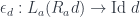
 \cong \mathcal{C}(a, R_b f) = \mathcal{C}(a, f b)](https://s0.wp.com/latex.php?latex=%5B%5Cmathcal%7BC%7D%2C%5Cmathbf%7BSet%7D%5D%28L_b+a%2C+f%29+%5Ccong+%5Cmathcal%7BC%7D%28a%2C+R_b+f%29+%3D+%5Cmathcal%7BC%7D%28a%2C+f+b%29&bg=ffffff&fg=29303b&s=0&c=20201002)


 translates to the function type


 . Product is functorial in both arguments so, in particular, we can define a functor

 (a.k.a., the exponential object
  ). The existence of this adjunction is what makes a category closed. You may recognize these two functors as, respectively, the writer and the reader functor. When the parameter

 , we’ll work with the comma category
  . Its objects are pairs
  , in which
  .
.

 while capturing all possible environments. The function object we are constructing is essentially a sum of all these closures, except that some of them are counted multiple times, so we need to perform some identifications. That’s what morphisms are for.
 in
in  that make the following triangles in
  commute.

 , or
, or  (
( is the unit of the product, so
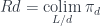
 is just the slice category
  of arrows to
  . The colimit of a diagram that has a terminal object is that terminal object. So, indeed, in this case, our construction produces a function object that is isomorphic to

 corresponds to the
 .
. there is a morphism
  that makes the following triangle commute:
 . We know for sure that
  of
of 
 . The comma category
  would then consist of pairs
  . The coproduct of all those environments is a good candidate for the function object

 satisfies at least one requirement of the function object: there is an implementation of
  . These are pairs
  that, among themselves, can factor out any

 and a morphism
  to satisfy that equation. Every
  and
and 
 to approximate the adjoint (thus skipping the equalizer part).

 .
. , where


 .
. .
. . In other words, these are all the arrows that emanate from
  to
to  is a morphism
  that makes the following triangle commute:
 , where
  that make the following diagram commute in

 that maps
  to
to 
 doesn’t necessarily cover the whole of
  : the left adjoint of
  must be the limit of the diagram
  in
in  .
.
 . In fact, this is the initial object in that category. If you pick any other object, say,
  , you can always find a morphism
  , which is just a leg, a projection, in the limiting cone that defines
 . We define the comma category
  and use
  to create the diagram whose limit is
  . We pick
  to be a projection in the limiting cone. We are guaranteed that
  under
under 

 :
:

 as the product of

 and construct a family
  of objects of
  . But in a comma category we also have morphisms between arrows. In fact they are the essential carriers of the structure of the comma category. Let’s have another look at these morphisms.
 and
and  . But if we restrict the factors
  (for arbitrary
  such that

 is continuous (small-limit preserving), and it satisfies the solution set condition, then
 are isomorphic

 ). Objects in the category of elements are pairs
  where
where  is an element of a set.
  is a morphism
  in
in  .
.
 . This is why you’ll see it written as an integral

 and terminating at a fixed object
  , so the comma category is just a category of elements for the functor
 :
:

 from some indexing category
  . The legs of a cocone are morphisms that connect the vertices of the diagram to the apex
 , we select an element of the hom-set
  , as a wire of the cocone. This is a selection of an element of a set (the hom-set) and, as such, can be described by a function from the singleton set
  . In other words, a wire is a member of
  . In fact, we can describe the whole cocone as a natural transformation between two functors, one of them being the constant functor
  . The set of cocones is then the set of natural transformations:
)](https://s0.wp.com/latex.php?latex=%5B%5Cmathcal%7BJ%7D%5E%7Bop%7D%2C+Set%5D%281%2C+%5Cmathcal%7BC%7D%28D+-%2C+c%29%29&bg=ffffff&fg=29303b&s=0&c=20201002)
![[J^{op}, Set]](https://s0.wp.com/latex.php?latex=%5BJ%5E%7Bop%7D%2C+Set%5D&bg=ffffff&fg=29303b&s=0&c=20201002) is the category of presheaves, that is functors from
is the category of presheaves, that is functors from  to
to  , with natural transformations as morphisms. As a bonus, we get the cocone triangle commuting conditions from naturality.
  with a more general functor
  . The result is a weighted colimit (or an indexed colimit, as Kelly calls it),
  . The set of weighted cocones is defined by natural transformations
)](https://s0.wp.com/latex.php?latex=%5B%5Cmathcal%7BJ%7D%5E%7Bop%7D%2C+Set%5D%28W%2C+%5Cmathcal%7BC%7D%28D+-%2C+c%29%29&bg=ffffff&fg=29303b&s=0&c=20201002)
) \cong \mathcal{C}(\mbox{colim}^W D, c)](https://s0.wp.com/latex.php?latex=%5B%5Cmathcal%7BJ%7D%5E%7Bop%7D%2C+Set%5D%28W%2C+%5Cmathcal%7BC%7D%28D+-%2C+c%29%29++%5Ccong++%5Cmathcal%7BC%7D%28%5Cmbox%7Bcolim%7D%5EW+D%2C+c%29&bg=ffffff&fg=29303b&s=0&c=20201002)


 as the sum of
 is, roughly speaking, like a bundle whose base is the category
  .
. 


![\begin{aligned} \mathcal{C}(\mbox{colim}^W D, c') & \cong [\mathcal{J}^{op}, Set]\big(W-, \mathcal{C}(D -, c')\big) \\ &\cong \int_j Set \big(W j, \mathcal{C}(D j, c')\big) \\ &\cong \int_j \mathcal{C}(W j \cdot D j, c') \\ &\cong \mathcal{C}(\int^j W j \cdot D j, c') \end{aligned}](https://s0.wp.com/latex.php?latex=%5Cbegin%7Baligned%7D++%5Cmathcal%7BC%7D%28%5Cmbox%7Bcolim%7D%5EW+D%2C+c%27%29+%26+%5Ccong+%5B%5Cmathcal%7BJ%7D%5E%7Bop%7D%2C+Set%5D%5Cbig%28W-%2C+%5Cmathcal%7BC%7D%28D+-%2C+c%27%29%5Cbig%29+%5C%5C+++%26%5Ccong+%5Cint_j+Set+%5Cbig%28W+j%2C+%5Cmathcal%7BC%7D%28D+j%2C+c%27%29%5Cbig%29+%5C%5C+++%26%5Ccong+%5Cint_j+%5Cmathcal%7BC%7D%28W+j+%5Ccdot+D+j%2C+c%27%29+%5C%5C+++%26%5Ccong+%5Cmathcal%7BC%7D%28%5Cint%5Ej+W+j+%5Ccdot+D+j%2C+c%27%29++%5Cend%7Baligned%7D+++&bg=ffffff&fg=29303b&s=0&c=20201002)

![[ \mathcal{C}^{op}, Set]\big(\mathcal{C}(-, x), H \big) \cong \int_c Set \big( \mathcal{C}(c, x), H c \big) \cong H x](https://s0.wp.com/latex.php?latex=%5B+%5Cmathcal%7BC%7D%5E%7Bop%7D%2C+Set%5D%5Cbig%28%5Cmathcal%7BC%7D%28-%2C+x%29%2C+H+%5Cbig%29+%5Ccong+%5Cint_c+Set+%5Cbig%28+%5Cmathcal%7BC%7D%28c%2C+x%29%2C+H+c+%5Cbig%29+%5Ccong+H+x&bg=ffffff&fg=29303b&s=0&c=20201002)


