Programming

Archived Posts from this Category

October 9, 2019

Fibrations, Cleavages, and Lenses

Posted by Bartosz Milewski under Programming
[2] Comments

In category theory, as in life, you spend half of your time trying to forget things, and half of the time trying to recover them. A morphism, the basic building block of every category, is like a defective isomorphism. It maps the initial state to the final state, but it provides no guarantees that you can recover the original. But it seems like this lossiness is what makes morphisms useful.

There are people who can memorize mathematical formulas perfectly but have no idea what they mean. And there are those who get just the gist of it, but can derive the rest when needed. Somehow understanding is related to lossy compression.

We can’t recover lost information. Once it’s gone, it’s gone. All we can do is to try to figure out what the original might have been like. In fact, knowing how the information was lost, we might be able to generate all possible inputs that could have led to a given output. It’s the closest we can get to inverting the uninvertible. This is the main idea behind fibrations.

Let me illustrate this concept with an example. Consider the function isEven:

isEven :: Integer -> Bool
isEven n = n `mod` 2 == 0

This function is definitely not invertible. If I only told you that the output was True, you couldn’t tell me what the input was. You could, however, give me the set of all inputs that could have produced this output: it’s the set of even numbers. We often call this set, which is the inverse image of True, a fiber over True. Similarly, the fiber over False is the set of odd numbers. In this case we only have only two fibers and they happen to be isomorphic.

Here’s a more interesting example. Consider a set of all lists of integers and a function that returns the length of a list: a natural number:

length :: [Integer] -> Nat

This function is not invertible, but it defines fibers over natural numbers. The fiber over zero is a one-element set that contains only the empty list. The fiber over 1 is the set of lists of length one (which is isomorphic to the set of integers). The fiber over 2 is a set of 2-element lists, or pairs of integers, and so on. You may recognize these fibers as length-indexed lists, or vectors. You can find them, for instance, in the Haskell Vec library or as Vect in Idris. These are not your typical data types, though. They are examples of dependent types–types that depend on values (here, natural numbers).

Notice that the name “length-indexed lists” suggests a slightly different interpretation of these types. You may think of them as families of types parameterized by natural numbers. This would suggest a mapping from elements of a set (natural numbers) to types. These two views are equivalent, but in category theory we try to avoid, if possible, talking about sets (and set elements in particular). The interpretation of dependent types as fibrations is more general, so let’s dig into fibrations.

As a generalization of functions like isEven or length, we’ll consider a morphism $\pi \colon e \to b$ , and call it a projection, since it projects each fiber down to one element. Our goal, though, is to define a fiber as the pre-image of an element in $b$ . But what’s an element? The closest we can get to defining an element in category theory is to consider a morphism $x$ from the terminal object $1$ . Such morphism is called a global element and, in $Set$ it really picks a single element from a (non-empty) set. Now we have two morphisms converging on $b$ : $\pi$ and $x$ . Conceptually, a fiber is a subobject $e_x$ of $e$ , which means that there must be a morphism $s$ that embeds $e_x$ in $e$ . Moreover, when this embedding is followed by the projection $\pi$ , it must produce the same element as $x$ . The best such object is given by a universal construction which, in this case, is a pullback.

Fig. 1.

(The exclamation mark stands for the unique morphism to the terminal object.) Incidentally, this is why a pullback is sometimes called a fiber product.

If fibers over all elements $x$ are isomorphic, the pair $(e, \pi)$ is, quite fittingly, called a fiber bundle. The object $b$ , from which the fibers sprout, is called the base. (Notice that lenght-indexed lists don’t form a bundle.)

Anything you can do with functions, you can do with functors, only better. So we can have a category $E$ , another category $B$ , and a functor $p \colon E \to B$ . Since a functor acts as a function on objects (modulo size issues), we can define a fiber as a set of objects in $E$ that are mapped to a single object in $B$ . The big question is, what do we do with morphisms? We have potentially lots of morphisms in $E$ that go between any two fibers, and which get projected down to a single hom-set in $B$ . If we want to invert $p$ , we have to design a procedure for lifting morphisms from $B$ to $E$ .

Here’s the idea: We would like each fiber to form a subcategory of $E$ , and we’d like to pick morphisms between fibers in such a way that $p^{-1}$ becomes a functor from $B$ to $Cat$ . In other words, we want $p^{-1}$ to map objects of $B$ to categories (the fibers), and morphisms of $B$ to functors between those categories. If this is too much to ask (which it often is), we’ll settle for $p^{-1}$ to be a pseudo-functor, which is a functor that preserves unit and composition only up to isomorphism. In fact the original construction (attributed to Grothendieck) produces a contravariant pseudo-functor. In this post I’ll describe the covariant version of this construction, which is called opfibration, and which is easier to explain.

The starting point of Grothendieck fibration is the recipe for lifting morphisms from the base category $B$ to the total category $E$ . There is a universal construction for doing that. The resulting morphisms are called opcartesian.

Let’s start with a morphism $f \colon a \to b$ in the base category and pick an arbitrary object $s$ (source) in the fiber over $a$ (hence $a = p s$ ). This will be the source of our opcartesian morphism. We have a lot of choices for the target. Strictly speaking, the target should be one of the objects over $b$ , and that’s what we are aiming for. However, a universal construction should look at a much larger pool of candidates, some of them with targets in other fibers. This pool enlargement helps narrow down the final choice with greater accuracy. (Remember, universal constructions are unique only up to isomorphism.)

The opcartesian morphism over $f$ , with the specified source $s$ , is a morphism $g \colon s \to t$ , such that $p g = f$ .

Fig. 2.

It must satisfy a universal property that I’m about to describe.

First, we pick an arbitrary object $x$ and a morphism $h \colon s \to x$ . This is supposed to be the competition for $g$ . When projected down to $B$ , it becomes $p h \colon a \to p x$ .

Fig. 3.

We are interested in the case when $p h$ factorizes through $f$ , that is, there is a morphism $u \colon b \to p x$ such that $p h = u \circ f$ . Whenever such factorization is possible in $B$ , we demand that there be a unique lifting of it to $E$ .

Fig. 4.

In other words, there exists a unique $\nu \colon t \to x$ such that $h = \nu \circ g$ and $p \nu = u$ .

If you find this definition a little confusing, you’re in good company. So let’s try a slightly different imagery that has more to do with the original ideas from algebraic topology. Think of objects as shapes. A morphism $f \colon a \to b$ is a proof that $b$ is a proper subset of $a$ , or that $a$ contains $b$ . A functor between two categories of shapes must map shapes to shapes in a way that preserves inclusion. It may map many shapes to one, so imagine that the shapes in the category $E$ are three-dimensional, and their projections using the functor $p$ are their flat shadows. Functoriality means that, if $s$ contains $t$ , then its shadow $a = p s$ contains $b = p t$ . Next, we introduce a new object $x$ that is contained inside $s$ , and the proof of that is $h \colon s \to x$ . It follows from functoriality that $a$ contains the shadow of $x$ .

Now suppose that this shadow falls inside the smaller $b$ (with the proof $u \colon b \to p x$ ).

Fig. 5.

Normally, this would not imply that $x$ is inside $t$ . It’s possible that (parts of) $x$ are sticking out below or above $t$ . Our universal condition demands that this cannot happen. There can be no room above or below $t$ — it’s a cylinder carved into $s$ . Universality guarantees that we get the absolutely optimal shape.

Now that we know what an opcartesian morphism is, we might ask the question, does it always exist? Given an arbitrary morphism $f \colon a \to b$ in $B$ and an object $s$ over $a$ , can we always find an opcartesian morphism $g \colon s \to t$ such that $t$ is over $b$ ? If we can, then we call the pair $(E, p \colon E \to B)$ an opfibration.

Here’s an interesting observation. You might wonder whether the definition of an opcartesian morphism isn’t overly complicated. Wouldn’t it be enough to restrict the pool of possible candidates to those morphisms whose target, the $x$ in our picture, was over $b$ , the target of $f$ ? This was, in fact, the original idea in the Grothendieck construction. The problem was that, with such definition, there was no guarantee that a composition of two opcartesian morphisms would be again opcartesian. The current definition makes that automatic.

Given an opfibration, we now face the opposite problem: there may be too many opcartesian morphisms. Remember, we wanted to (a) make fibers into subcategories of $E$ and (b) use opcartesian morphisms to define functors between them. The first part is relatively easy: a fiber $E_a$ has, as objects, those objects of $E$ whose projection is $a$ . We select as morphisms in $E_a$ those morphisms that project down to identity, $id_a$ (notice that we ignore other endomorphism $a \to a$ ). These are called vertical morphisms. But to define functors between fibers we need to map each object of one fiber to exactly one object in the other fiber (and the same for vertical morphisms). Think of this as transporting objects between fibers. In a fibered category, we could use opcartesian morphisms for transport. Any time two objects are connected in the base by a morphism, we have a bunch of opcartesian morphisms over it starting from every single object in the source fiber. We could use them to try to define a functor between fibers.

But in general we have more than one opcartesian morphism between a source object in one fiber and candidate target objects in the other fiber. But we can design a procedure to pick one (if you’re into set theory, you’ll notice that we have to use the Axiom of Choice). Such choice is called an opcleavage, and the resulting construction is called cloven opfibration.

Formally, an opcleavage is described by a function $\kappa (f, s)$

Fig. 6.

It takes a morphism $f \colon a \to b$ and an object $s$ (such that $p s = a$ ), and produces an object $t$ (such that $p t = b$ ), which is the target of some opcartesian morphism $s \to t$ . This is exactly the morphism selected by opcleavage.

The universal construction of opcartesian morphisms can then be used to define the mapping of vertical morphisms thus completing the definition of a functor between fibers.

A geometric intuition is that an opcleavage provides a way of transporting objects in the horizontal direction. Vertical morphisms transport objects vertically, and the functors defined by the opcleavage transport them horizontally, in such a way that their shadows follow the arrows in the base. The origin of this intuition goes back to differential geometry, where one is able to define continuous paths in the base manifold and use them to transport objects, such as vectors, between fibers. Category theory lets us abstract away continuity (and differentiability) from this picture. You might also see transport used in homotopy type theory, with paths standing for equality proofs.

Now, remember what I said about the composition of opcartesian morphisms resulting in an opcartesian morphism? Unfortunately, once we start picking individual morphisms to construct an opcleavage, this compositionality might be lost. The composition of any two morphisms from the selected pool is still opcartesian, but it’s not necessarily part of the opcleveage. This is why we might have to relax compositionality and embrace pseudofunctors.

But sometimes an opcleavage preserves compositionality. We call this situation split opfibration. It must satisfy these two conditions:

$\kappa (id_a, s) = id_s$

$\kappa (f', s') \circ \kappa(f, s) = \kappa(f' \circ f, s)$

for any $f \colon a \to b$ and $f' \colon b \to c$ .

A split opfibration defines a functor $B \to Cat$ , which maps objects from the base category to fibers seen as categories; and morphisms from the base category to functors between those fibers. So defined functor may be interpreted as an attempt at inverting the original projection $p \colon E \to B$ .

If the splitting conditions are satisfied only up to isomorphism, we get a pseudofunctor $B \to Cat$ . This makes things more complicated but also more interesting. It means that horizontal transport depends on the path. In particular, transport along a closed path–a chain of morphisms in the base that compose to identity–may produce an object that’s different from (albeit isomorphic to) the starting object. In differential geometry we would say that the space has non-zero curvature.

Interestingly, this procedure of generating split opfibrations has its inverse. Given a functor $B \to Cat$ it’s possible to reconstruct the total category $E$ and a projection $p \colon E \to B$ . This is called the Grothendieck construction.

Since our new slogan is “lenses are everywhere,” it should come as no big surprise that a split opfibration may be seen as a type of a lens. The projection corresponds to view or get. It extracts $a$ , the focus of the lens, out of $s$ . The opcleavage part of opfibration, $\kappa(f, s)$ corresponds to put or, more precisely to over. It takes a morphism that modifies the focus from $a$ to $b$ and it takes the object $s$ , and produces the new object $t$ . In programming, get and put are just functions between sets, here they are object mappings of two functors, but the similarity is hard to ignore.

Acknowledment

I’m grateful to Bryce Clarke for reading the draft and helpful comments.

Papers to read

Johnson, Rosebrugh, and Wood, Lenses, fibrations and universal translations
Johnson and Rosebrugh, Delta lenses and opfibrations

September 20, 2019

The Power of Adjunctions

Posted by Bartosz Milewski under Category Theory, Monads, Programming
[15] Comments

In my previous blog post, Programming with Universal Constructions, I mentioned in passing that one-to-one mappings between sets of morphisms are often a manifestation of adjunctions between functors. In fact, an adjunction just extends a universal construction over the whole category (or two categories, in general). It combines the mapping-in with the mapping-out conditions. One functor (traditionally called the left adjoint) prepares the input for mapping out, and the other (the right adjoint) prepares the output for mapping in. The trick is to find a pair of functors that complement each other: there are as many mapping-outs from one functor as there are mapping-ins to the other functor.

To gain some insight, let’s dig deeper into the examples from my previous post.

The defining property of a product was the universal mapping-in condition. For every object $c$ equipped with a pair of morphisms going to, respectively, $a$ and $b$ , there was a unique morphism $h$ mapping $c$ to the product $a \times b$ . The commuting condition ensured that the correspondence went both ways, that is, given an $h$ , the two morphisms were uniquely determined.

A pair of morphisms can be seen as a single morphism in a product category $C\times C$ . So, really, we have an isomorphism between hom-sets in two categories, one in $C\times C$ and the other in $C$ . We can also define two functors going between these categories. An arbitrary object $c$ in $C$ is mapped by the diagonal functor $\Delta$ to a pair $\langle c, c\rangle$ in $C\times C$ . That’s our left functor. It prepares the source for mapping out. The right functor maps an arbitrary pair $\langle a, b\rangle$ to the product $a \times b$ in $C$ . That’s our target for mapping in.

The adjunction is the (natural) isomorphism of the two hom-sets:

$(C\times C)(\Delta c, \langle a, b\rangle) \cong C(c, a \times b)$

Let’s develop this intuition. As usual in category theory, an object is defined by its morphisms. A product is defined by the mapping-in property, the totality of morphisms incoming from all other objects. Hence we are interested in the hom-set between an arbitrary object $c$ and our product $a \times b$ . This is the right hand side of the picture. On the left, we are considering the mapping-out morphism from the object $\langle c, c \rangle$ , which is the result of applying the functor $\Delta$ to $c$ . Thus an adjunction relates objects that are defined by their mapping-in property and objects defined by their mapping-out property.

Another way of looking at the pair of adjoint functors is to see them as being approximately the inverse of each other. Of course, they can’t, because the two categories in question are not isomorphic. Intuitively, $C\times C$ is “much bigger” than $C$ . The functor that assigns the product $a \times b$ to every pair $\langle a, b \rangle$ cannot be injective. It must map many different pairs to the same (up to isomorphism) product. In the process, it “forgets” some of the information, just like the number 12 forgets whether it was obtained by multiplying 2 and 6 or 3 and 4. Common examples of this forgetfulness are isomorphisms such as

$a \times b \cong b \times a$

$(a \times b) \times c \cong a \times (b \times c)$

Since the product functor loses some information, its left adjoint must somehow compensate for it, essentially by making stuff up. Because the adjunction is a natural transformation, it must do it uniformly across the whole category. Given a generic object $c$ , the only way it can produce a pair of objects is to duplicate $c$ . Hence the diagonal functor $\Delta$ . You might say that $\Delta$ “freely” generates a pair. In almost every adjunction you can observe this interplay of “freeness” and “forgetfulness.” I’m using these therm loosely, but I can be excused, because there is no formal definition of forgetful (and therefore free or cofree) functors.

Left adjoints often create free stuff. The mnemonic is that “the left” is “liberal.” Right adjoints, on the other hand, are “conservative.” They only use as much data as is strictly necessary and not an iota more (they also preserve limits, which the left adjoints are free to ignore). This is all relative and, as we’ll see later, the same functor may be the left adjoint to one functor and the right adjoint to another.

Because of this lossiness, a round trip using both functors doesn’t produce an identity. It is however “related” to the identity functor. The combination left-after-right produces an object that can be mapped back to the original object. Conversely, right-after-left has a mapping from the identity functor. These two give rise to natural transformations that are called, respectively, the counit $\varepsilon$ and the unit $\eta$ .

Here, the combination diagonal functor after the product functor takes a pair $\langle a, b\rangle$ to the pair $\langle a \times b, a \times b\rangle$ . The counit $\varepsilon$ then maps it back to $\langle a, b\rangle$ using a pair of projections $\langle \pi_1, \pi_2\rangle$ (which is a single morphism in $C \times C$ ). It’s easy to see that the family of such morphisms defines a natural transformation.

If we think for a moment in terms of set elements, then for every element of the target object, the counit extracts a pair of elements of the source object (the objects here are pairs of sets). Note that this mapping is not injective and, therefore, not invertible.

The other composition–the product functor after the diagonal functor–maps an object $c$ to $c \times c$ . The component of the unit natural transformation, $\eta_c \colon c \to c \times c$ , is implemented using the universal property of the product. Indeed, such a morphism is uniquely determined by a pair of identity morphsims $\langle id_c, id_c \rangle$ . Again, when we vary $c$ , these morphisms combine to form a natural transformation.

Thinking in terms of set elements, the unit inserts an element of the set $c$ in the target set. And again, this is not an injective map, so it cannot be inverted.

Although in an arbitrary category we cannot talk about elements, a lot of intuitions from $Set$ carry over to a more general setting. In a category with a terminal object, for instance, we can talk about global elements as mappings from the terminal object. In the absence of the terminal object, we may use other objects to define generalized elements. This is all in the true spirit of category theory, which defines all properties of objects in terms of morphisms.

Every construction in category theory has its dual, and the product is no exception.

A coproduct is defined by a mapping out property. For every pair of morphisms from, respectively, $a$ and $b$ to the common target $c$ there is a unique mapping out from the coproduct $a + b$ to $c$ . In programming, this is called case analysis: a function from a sum type is implemented using two functions corresponding to two cases. Conversely, given a mapping out of a coproduct, the two functions are uniquely determined due to the commuting conditions (this was all discussed in the previous post).

As before, this one-to-one correspondence can be neatly encapsulated as an adjunction. This time, however, the coproduct functor is the left adjoint of the diagonal functor.

The coproduct is still the “forgetful” part of the duo, but now the diagonal functor plays the role of the cofree funtor, relative to the coproduct. Again, I’m using these terms loosely.

The counit now works in the category $C$ and it “extracts a value” from the symmetric coproduct of $c$ with $c$ . It does it by “pattern matching” and applying the identity morphism.

The unit is more interesting. It’s built from two injections, or two constructors, as we call them in programming.

I find it fascinating that the simple diagonal functor can be used to define both products and coproducts. Moreover, using terse categorical notation, this whole blog post up to this point can be summarized by a single formula.

That’s the power of adjunctions.

There is one more very important adjunction that every programmer should know: the exponential, or the currying adjunction. The exponential, a.k.a. the function type, is the right adjoint to the product functor. What’s the product functor? Product is a bifunctor, or a functor from $C \times C$ to $C$ . But if you fix one of the arguments, it just becomes a regular functor. We’re interested in the functor $(-) \times b$ or, more explicitly:

$(-) \times b : a \to a \times b$

It’s a functor that multiplies its argument by some fixed object $b$ . We are using this functor to define the exponential. The exponential $a^b$ is defined by the mapping-in property. The mappings out of the product $c \times b$ to $a$ are in one to one correspondence with morphisms from an arbitrary object $c$ to the exponential $a^b$ .

$C(c \times b, a) \cong C(c, a^b)$

The exponential $a^b$ is an object representing the set of morphisms from $b$ to $a$ , and the two directions of the isomorphism above are called curry and uncurry.

This is exactly the meaning of the universal property of the exponential I discussed in my previous post.

The counit for this adjunction extracts a value from the product of the function type (the exponential) and its argument. It’s just the evaluation morphism: it applies a function to its argument.

The unit injects a value of type $c$ into a function type $b \to c \times b$ . The unit is just the curried version of the product constructor.

I want you to look closely at this formula through your programming glasses. The target of the unit is the type:

b -> (c, b)

You may recognize it as the state monad, with b representing the state. The unit is nothing else but the natural transformation whose component we call return. Coincidence? Not really! Look at the component of the counit:

(b -> a, b) -> a

It’s the extract of the Store comonad.

It turns out that every adjunction gives rise to both a monad and a comonad. Not only that, every monad and every comonad give rise to adjunctions.

It seems like, in category theory, if you dig deep enough, everything is related to everything in some meaningful way. And every time you revisit a topic, you discover new insights. That’s what makes category theory so exciting.

July 4, 2019

Filtered Colimits

Posted by Bartosz Milewski under Programming
1 Comment

Previously we were exploring universal constructions for products, coproducts, and exponentials. In particular, we were able to prove the distributive law:

$(a + b) \times c \cong a \times c + b \times c$

The power of this law is that it relates the mapping-in universal construction (product on the left) with the mapping-out one (coproduct on the right). If you take into account that products and coproducts are just special cases of limits and colimits, you may ask a more general question: under what conditions limits commute with colimits. In a cartesian closed category a product of sums is not equal to the sum of products:

$(a + b) \times (c + d) \ncong a \times c + b \times d$

So, in general, products don’t commute with coproducts. But if you replace coproducts with a special kind of colimits, then it can be shown that:
Theorem.
In $Set$ , filtered colimits commute with finite limits.

In this post I’ll try to explain these terms and provide some intuition why it works and how filtered colimits are related to the more traditional notion of limits that we know from calculus.

Limits

Let’s start with limits. They are like products, except that, instead of just two objects at the bottom, you have any number of objects plus a bunch of morphisms between them. That’s called a diagram. Then you have an apex with arrows going down to all the objects in the diagram; and you get what is called a cone. If you have morphisms in your diagram, they form triangles. These triangles must commute. For instance, in Fig 1, we have:

$g \circ \pi_1 = \pi_3$

Fig. 1. A cone

This means that not all projections are independent–that you may obtain one projection from another by post-composing it with a morphism from the diagram. In Fig 1, for instance, you may extract a value of $c$ either directly using $\pi_3$ or by applying $g$ to the result of $\pi_1$ .

A limit is defined as the universal cone with the apex $Lim$ . It means that, if you have any other cone with some apex $c$ , built over the same diagram, there is a unique morphism $h$ from $c$ to $Lim$ that makes all the triangles commute. For instance, in Fig 2, one of the commuting conditions is:

$\pi_1 \circ h = f_1$

and so on. We’ve seen similar commuting conditions in the definition of the product.

Fig. 2. A universal cone

If you think of $Lim$ in this example as a data structure, you would implement it as a product of $a_1$ , $a_2$ , and $a_3$ , together with two functions:

$g_3 : a_1 \to a_3$

$g_2 : a_1 \to a_2$

But because of the commuting conditions, the three values stored in $Lim$ cannot be independent. If you pick a value for $a_1$ , then the values for $a_2$ and $a_3$ are uniquely determined.

A limit, just like a product, is defined by a mapping-in property. If you want to define a morphism from some $c$ to $Lim$ , you need to provide three morphisms $f_1$ , $f_2$ , and $f_3$ . However, unlike in the case of a product, these morphisms must satisfy some commuting conditions. Here, $f_3$ must be equal to $g_3 \circ f_1$ and $f_2 = g_2 \circ f_1$ . So, really, you only need to define $f_1$ , and that uniquely determines $h$ . This is why the cones in Fig 2 can be simplified, as shown in Fig 3.

Fig. 3. A simplified universal cone

Notice that the diagram essentially forms a subcategory inside the category $C$ , even if we don’t explicitly draw all the identity morphisms or all the compositions. This is because triangles built by composing commuting triangles are again commuting. It therefore makes sense to define a diagram as a functor $F$ from an (often much smaller) index category $J$ to $C$ . In our case it would be a category with just three objects, $j_1$ , $j_2$ , $j_3$ , and two non-identity morphisms. (The diagram category for the product is even simpler: just two objects, no non-trivial morphisms.)

The properties of the diagram category determine the nature of cones and the nature of the limits. For instance, functors from a finite category will produce finite limits.

Fig. 4. Diagram category $J$

The diagram category $J$ in our example has a very peculiar property: it has a cone for every pair of objects (it’s a cone inside $J$ , not to be confused with the cone in $C$ ). For instance, the pair $j_2$ , $j_3$ is part of the cone with the apex $j_1$ . This is also the apex for the (somewhat degenerate) cone based on $j_1$ and $j_2$ (with or without the connecting morphism). A category in which there is a cone for every finite subdiagram is called cofiltered. Limits defined by functors from cofiltered categories are called cofiltered limits.

The intuition is that cofiltered categories exhibit some kind of ordering. You may think of $j_1$ as a lower bound of $j_2$ and $j_3$ . Following these bounds, you might eventually get to some kind of roots–here it’s the object $j_1$ –and these roots will dictate the behavior of cones and the behavior of limits. Things get really interesting when the diagram category is infinite, because then there is no guarantee that you’ll ever reach a root. There is, for instance, no smallest (negative) integer, even though integers are ordered. You can begin to see parallels with traditional limits, like:

$\lim_{j \to -\infty} a_j$

That’s where these ideas originally came from.

Limits in the category of sets have a particularly simple interpretation. In $Set$ , we can use functions from the terminal object–the singleton set–to pick individual set elements.

Fig. 5. Elements of the limit

For every selection in Fig 5. of $x_1$ , $x_2$ , $x_3$ there is a unique $h(x_1, x_2, x_3)$ that picks an element in $Lim$ . But a selection of $x_1$ , $x_2$ , $x_3$ is nothing but a cone with the apex $1$ . So there is a one-to-one correspondence between elements of $Lim$ and such cones. In other words, $Lim$ is a set of apex-1 cones.

Colimits

Colimits are dual to limits–you get them by inverting all the arrows. So, instead of projections, you get injections, and the universal condition defines a mapping out of a colimit (see Fig 6).

Fig. 6. A universal cocone

If you look at the colimit as a data structure, it is similar to a coproduct, except that not all the injections are independent. In the example in Fig 6, $i_3$ and $i_2$ are determined by pre-composing $i_1$ with $g_3$ and $g_2$ , respectively. It’s not clear how to implement a colimit in Haskell, so here’s a pseudo-Haskell attempt using imaginary dependent-type syntax:

  data Colim a1 a2 a3 (g2 :: a2 -> a1) (g3 :: a3 -> a1) =
           = A1 a1 | A2 a2 | A3 a3

To deconstruct this colimit, you only need to provide one function $f_1 : a_1 \to c$ .

  h :: (a1 -> c) -> Colim a1 a2 a3 g2 g3 -> c
  h f1 (A1 a1)    = f1 a1
  h f1 (A2 a2) = f1 (g2 a2)
  h f1 (A3 a3) = f1 (g3 a3)

Granted, in a lazy language like Haskell, this would be an overkill way to store essentially just one value.

A colimit in the category of sets simplifies to a disjoint union of sets, in which some elements are identified. Suppose that the colimit $Colim_J F$ is defined by some diagram category $J$ and a functor $F : J \to Set$ . Each object $j$ in $J$ produces a set $F j$ .

Fig. 7. Colimit in Set. On the left, the diagram category $J$ .

The disjoint union of all these sets is a set whose elements are the pairs $(x, j)$ where $x \in F j$ . (Notice that the sets may overlap, but each element from the overlap will be counted as many times as the number of sets it belongs to.) Coproduct injections are then functions that take an element $x \in F j$ and map it into an element $(x, j) \in Colim_J F$ . But that doesn’t take into account the presence of morphisms in the diagram. These morphisms are mapped to functions between corresponding sets. For instance, in Fig 7, we can take an element $x \in F j_2$ . It is injected, using $i_2$ , as an element $(x, j_2) \in Colim_J F$ . But there is another path from $F j_2$ that uses $F g_2$ followed by $i_1$ . That produces $((F g_2) x, j_1)$ . If the triangle is to commute, these two must be equal. So in the actual colimit, they must be identified. In general, any two elements of the disjoint union that satisfy this relation:

$(x, j) \rightsquigarrow (x', j')\;\; \text{if}\;\; \exists_{g : j \to j'} (F g) x = x'$

must be identified. This is not an equivalence relation, but it can be extended to one (by first symmetrizing it, and then making it transitive again). A colimit is then a quotient of the disjoint union by this equivalence.

As before, I chose this example to illustrate a special type of a diagram. This is a diagram that can be obtained using a functor from a filtered category. A filtered category has this property that for any finite subdiagram, there is a cocone under it. Here, for instance, the subdiagram formed by $j_2$ and $j_3$ has a cocone with the apex $j_1$ . Again, you may think of $j_1$ as a kind of upper bound of $j_2$ and $j_3$ . If the filtered category is finite, following upper bounds will eventually lead you to some roots. And in Set, the equivalence relation will allow you shift all the elements down to those roots. But in an infinite case (think natural numbers) there may be no largest element–no root. And that brings filtered colimits closer to the intuition we have for limits in calculus. In fact, all the interesting filtered colimits are based on infinite diagrams.

Commuting Limits and Colimits

What does it mean for a limit to commute with a colimit? A single colimit is generated by a functor from some index category $I \to C$ . What we need is a bunch of such colimits so that we can take a limit over those. Therefore we need a bunch of functors $I \to C$ . Moreover, those colimits have to form a diagram. So we need another index category $J$ to parameterize those functors. Altogether, we need a functor of two arguments:

$F : I \times J \to C$

It follows that, for any given $j$ in $J$ we have a functor $F(-, j) : I \to C$ . We can take a colimit of that. Then we gather those colimits into a diagram whose shape is defined by $J$ , and then take its limit. We get:

$Lim_J (Colim_I F)$

Alternatively, when we fix some $i$ in $I$ , we get a functor $F(i, -) : J \to C$ . We can take a limit of that. Then we can gather all those limits and form a diagram whose shape is defined by $I$ . Finally we can take a colimit of that:

$Colim_I (Lim_J F)$

Fig. 8. Commuting limits (red diagram of shape $J$ ) and colimits (black diagram of shape $I$ )

It’s not difficult to construct the mapping:

$Colim_I (Lim_J F) \to Lim_J (Colim_I F)$

using the universal property, since the colimit has the mapping-out property. It’s the other way around that’s tricky. But it always works in the special case when $I$ is filtered, $J$ is finite, and $C$ is $Set$ .

Here’s the sketch of this amazing proof, which you can find in Saunders Mac Lane’s Categories for the Working Mathematician.

Since the target of the functor is Set, it might help to visualize its image as a rectangular array of sets. A fixed $j$ picks up a row of such sets, whereas a fixed $i$ picks up a column. Because we are dealing with sets, we can try to define the mapping:

$Lim_J (Colim_I F) \to Colim_I (Lim_J F)$

pointwise. Let’s pick an element of the limit on the left. As we’ve established earlier, a limit in Set is a set of apex-1 cones. So let’s pick one such cone. It’s just a selection of elements from a bunch of colimits.

As we’ve seen before, a colimit in Set is a discriminated union with some identifications. So our apex-1 cone will pick a set of representatives, one per colimit, say $(x_n, i_n)$ . Any time there is a morphism $g : i_n \to i'_n$ , we can replace one representative with another $(g (x_n), i'_n)$ . The intuition is that we can slide the representatives horizontally within each row along morphisms.

If $I$ is a filtered category, then for any finite number of objects $i_n$ , we can always find a common root (it will be the apex $i$ of a cocone formed by $i_n$ in $I$ ). So we can slide all the representatives to a single column. In other words, our cone can be brought to a set of representatives $(y_n, i)$ , with a common $i$ .

Fig. 9. A single cone after shifting representatives from all colimits to a common column

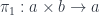
But that’s just a cone over $J$ . It’s an element of $Lim_J F$ . And we can inject it into a colimit over $I$ to get an element of $Colim_I (Lim_J F)$ . We have thus defined our mapping.

Conclusion

If you didn’t get the proof the first time, don’t get discouraged. Take a break, sleep over it, and then read it slowly again. Make sure you have internalized all the definitions. Draw your own pictures. The two major tricks are: (1) visualizing an element of a limit as a cone originating from the singleton set, and (2) the idea of sliding the elements of multiple colimits to a common column.

The importance of this theorem is that it tells you when and how you can define mappings out of limits. For instance, how to define functions from a product or from an end.

Acknowledgment

I’m grateful to Derek Elkins for correcting mistakes in the original version of this post.

July 3, 2019

Programming with Universal Constructions

Posted by Bartosz Milewski under Programming
1 Comment

As functional programmers we are interested in functions. Category theorists are similarly interested in morphisms. There is a slight difference in approach, though. A programmer must implement a function, whereas a mathematician is often satisfied with the proof of existence of a morphism (unless said mathematician is a constructivist). Category theory if full of such proofs. It turns out that many of these proofs can be converted to code, often resulting in quite unexpected encodings.

A lot of objects in category theory are defined using universal constructions and universality is used all over the place to show the existence (as a rule: unique, up to unique isomorphism) of morphisms between objects.

There are two major types of universal constructions: the ones asserting the mapping-in property, and the ones asserting the mapping-out property. For instance, the product has the mapping-in property.

Product

Recall that a product of two objects $a$ and $b$ is an object $a \times b$ together with two projections:

$\pi_1 : a \times b \to a$

$\pi_2 : a \times b \to b$

This object must satisfy the universal property: for any other object $c$ with a pair of morphisms:

$f : c \to a$

$g : c \to b$

there exists a unique morphism $h : c \to a \times b$ such that:

$f = \pi_1 \circ h$

$g = \pi_2 \circ h$

In other words, the two triangles in Fig 1 commute.

Fig. 1. Universality of the product

This universal property can be used any time you need to find a morphism that’s mapping into the product, and it can actually produce code.

For instance, let’s say you want to find a morphism from the terminal object $1$ to $a \times b$ . All you need is to define two morphisms $x : 1 \to a$ and $y : 1 \to b$ . This is not always possible, but if it is, you are guaranteed the existence of a morphism $h : 1 \to a \times b$ (Fig 2).

Fig. 2. Global element of a product

Morphisms from the terminal object are called global elements, so we have just shown that, as long as $a$ and $b$ have global elements, say $x$ and $y$ , their product has a global element too. Moreover the projection $\pi_1$ of this global element is the same as $x$ , and $\pi_2$ is the same as $y$ . In other words, an element of a product is a pair of elements. But you probably knew that.

The universal construction of the product is implemented as an operator in Haskell:

  (&&&) :: (c->a) -> (c->b) -> (c -> (a, b))

We can also go the other way: given a mapping-in $h : c \to a \times b$ , we can always extract a pair of morphisms:

$f = \pi_1 \circ h$

$g = \pi_2 \circ h$

This bijection between $h$ and a pair of morphisms $(f, g)$ is in fact an adjunction.

You might think this kind of reasoning is very different from what programmers do, but it’s not. Here’s one possible definition of a product in Haskell (besides the built-in one, (,)):

  data Product a b = MkProduct { fst :: a
                               , snd :: b }

It is in one-to-one correspondence with what I’ve just explained. The two functions fst and snd are $\pi_1$ and $\pi_2$ , and MkProduct corresponds to our $h : 1 \to a \times b$ . The categorical definition is just a different, much more general, way of saying the same thing.

Here’s another application of universality: Show that product is functorial. Suppose that you have a pair of morphisms:

$f : a \to a'$

$g : b \to b'$

and you want to lift them to a morphism:

$h : a \times b \to a' \times b'$

Since we are dealing with products, we should use the mapping-in property. So we draw the universality diagram for the target $a' \times b'$ , and put the source $a \times b$ at the top. The pair of functions that fits the bill is $(f \circ \pi_1, g \circ \pi_2)$ (Fig 3).

Fig. 3. Functoriality of the product

The universal property gives us, uniquely, the $h$ , which is usually written simply as $f \times g$ .

Exercise for the reader: Show, using universality, that categorical product is symmetric.

Coproduct

The coproduct, being the dual of the product, is defined by the universal mapping-out property, see Fig 4.

Fig. 4. Universality of the coproduct

So if you need a morphism from a coproduct $a + b$ to some $c$ , it’s enough to define two morphisms:

$f : a \to c$

$g : b \to c$

This universal property may also be restated as the isomorphism between pairs of morphisms $(f, g)$ and morphisms of the type $a+b \to c$ (so there is, in fact, a corresponding adjunction).

This is easily illustrated in Haskell:

  h :: Either a b -> c
  h (Left a)  = f a
  h (Right b) = g b

Here Left and Right correspond to the two injections $i_1$ and $i_2$ . There is a convenient function in Haskell that encapsulates this universal construction:

  either :: (a->c) -> (b->c) -> (Either a b -> c)

Exercise for the reader: Show that coproduct is functorial.

So next time you ask yourself, what can I do with a universal construction? the answer is: use it to define a morphism, either mapping in or mapping out of your construct. Why is it useful? Because it decomposes a problem into smaller problems. In the examples above, the problem of constructing one morphism $h$ was nicely decomposed into defining $f$ and $g$ separately.

The flip side of this is that there is no simple way of defining a mapping out of a product or a mapping into a coproduct.

Distributive Law

For instance, you might wonder if the familiar distributive law:

$(a + b) \times c \cong a \times c + b \times c$

holds in an arbitrary category that defines products and coproducts (so called bicartesian category). You can immediately see that defining a morphism from right to left is easy, because it involves the mapping out of a coproduct. All we need is to define a pair of morphisms leading to the common target (Fig 5):

$f : a \times c \to (a + b) \times c$

$g : b \times c \to (a + b) \times c$

Fig. 5. Right to left proof

The trick is to take advantage of the functoriality of the product, which we have already established, and use it to implement $f$ and $g$ as:

$f = i_1 \times id_c$

$g = i_2 \times id_c$

But if you try to construct a proof in the other direction, from left to right, you’re stuck, because it would require the mapping out of a product. So the distributive property does not hold in general.

“Wait a moment!” I hear you say, “I can easily implement it in Haskell.”

  f :: (Either a b, c) -> Either (a, c) (b, c)
  f (Left a, c)  = Left  (a, c)
  f (Right b, c) = Right (b, c)

Exponential

That’s correct, but Haskell does a little cheating behind the scenes. You can see it clearly when you convert this code to point free notation (I’ll explain later how I figured it out):

  f = uncurry (either (curry Left) (curry Right))

I want to direct your attention to the use of curry and uncurry. Currying is the application of another universal construction, namely that of the exponential object $c^b$ , representing the function type b -> c. This is exactly the construction that provides the missing mapping out of a product, (a, b) -> c. Here we go:

  uncurry :: (c -> (a -> b)) -> ((c, a) -> b)

Categorically, we have the bijection between morphisms (again, a sign of an adjunction):

$h : c \to b^a$

$f : c \times a \to b$

Universality tells us that for every $c$ and $f$ there is a unique $h$ in Fig 6 (and vice versa). The arrow $h \times id_a$ is the lifting of the pair $(h, id_a)$ by the product functor (we’ve established the functoriality of the product earlier).

Fig. 6. Universality of the exponential

Not every category has exponentials–the ones that do are called cartesian closed (cartesian, because they must also have products).

So how does the fact that we have exponentials in Haskell help us here? We are trying to define a mapping out of a product:

$f : (a + b) \times c \to a \times c + b \times c$

Here’s where the exponential saves the day. This mapping exists if we can define another mapping:

$h : (a + b) \to (a \times c + b \times c)^c$

see Fig 7.

Fig. 7. Uncurrying

This morphism, in turn, is easy to define, because it involves a mapping out of a sum. We just need a pair of morphisms:

$h_1 : a \to (a \times c + b \times c)^c$

$h_2 : b \to (a \times c + b \times c)^c$

We can define the first morphism using the universal property of the exponential, picking the injection $i_1$ :

Fig. 8. Defining $h_1$

This translates to Haskell as h1 = curry Left. Similarly for $h_2$ we get curry Right.

We can now combine all these diagrams into a single point-free definition, and that’s exactly how I came up with the original code:

  f = uncurry (either (curry Left) (curry Right))

Notice that curry is used to get from $f$ to $h$ , and uncurry from $h$ to $f$ in the original diagram.

Products and coproducts are examples of more general constructions called limits and colimits. Importantly, the universal property of limits can be used to define the mapping-in morphisms, whereas the universal property of colimits allows us to define the mapping-out morphisms. I’ll talk more about it in the upcoming post.

March 27, 2019

Promonads, Arrows, and Einstein Notation for Profunctors

Posted by Bartosz Milewski under Category Theory, Haskell, Monads, Programming
1 Comment

I’ve been working with profunctors lately. They are interesting beasts, both in category theory and in programming. In Haskell, they form the basis of profunctor optics–in particular the lens library.

Profunctor Recap

The categorical definition of a profunctor doesn’t even begin to describe its richness. You might say that it’s just a functor from a product category $\mathbb{C}^{op}\times \mathbb{D}$ to $Set$ (I’ll stick to $Set$ for simplicity, but there are generalizations to other categories as well).

A profunctor $P$ (a.k.a., a distributor, or bimodule) maps a pair of objects, $c$ from $\mathbb{C}$ and $d$ from $\mathbb{D}$ , to a set $P(c, d)$ . Being a functor, it also maps any pair of morphisms in $\mathbb{C}^{op}\times \mathbb{D}$ :

$f\colon c' \to c$
$g\colon d \to d'$

to a function between those sets:

$P(f, g) \colon P(c, d) \to P(c', d')$

Notice that the first morphism $f$ goes in the opposite direction to what we normally expect for functors. We say that the profunctor is contravariant in its first argument and covariant in the second.

But what’s so special about this particular combination of source and target categories?

Hom-Profunctor

The key point is to realize that a profunctor generalizes the idea of a hom-functor. Like a profunctor, a hom-functor maps pairs of objects to sets. Indeed, for any two objects in $\mathbb{C}$ we have the set of morphisms between them, $C(a, b)$ .

Also, any pair of morphisms in $\mathbb{C}$ :

$f\colon a' \to a$
$g\colon b \to b'$

can be lifted to a function, which we will denote by $C(f, g)$ , between hom-sets:

$C(f, g) \colon C(a, b) \to C(a', b')$

Indeed, for any $h \in C(a, b)$ we have:

$C(f, g) h = g \circ h \circ f \in C(a', b')$

This (plus functorial laws) completes the definition of a functor from $\mathbb{C}^{op}\times \mathbb{C}$ to $Set$ . So a hom-functor is a special case of an endo-profunctor (where $\mathbb{D}$ is the same as $\mathbb{C}$ ). It’s contravariant in the first argument and covariant in the second.

For Haskell programmers, here’s the definition of a profunctor from Edward Kmett’s Data.Profunctor library:

class Profunctor p where
  dimap :: (a' -> a) -> (b -> b') -> p a b -> p a' b'

The function dimap does the lifting of a pair of morphisms.

Here’s the proof that the hom-functor which, in Haskell, is represented by the arrow ->, is a profunctor:

instance Profunctor (->) where
  dimap ab cd bc = cd . bc . ab

Not only that: a general profunctor can be considered an extension of a hom-functor that forms a bridge between two categories. Consider a profunctor $P$ spanning two categories $\mathbb{C}$ and $\mathbb{D}$ :

$P \colon \mathbb{C}^{op}\times \mathbb{D} \to Set$

For any two objects from one of the categories we have a regular hom-set. But if we take one object $c$ from $\mathbb{C}$ and another object $d$ from $\mathbb{D}$ , we can generate a set $P(c, d)$ . This set works just like a hom-set. Its elements are called heteromorphisms, because they can be thought of as representing morphism between two different categories. What makes them similar to morphisms is that they can be composed with regular morphisms. Suppose you have a morphism in $\mathbb{C}$ :

$f\colon c' \to c$

and a heteromorphism $h \in P(c, d)$ . Their composition is another heteromorphism obtained by lifting the pair $(f, id_d)$ . Indeed:

$P(f, id_d) \colon P(c, d) \to P(c', d)$

so its action on $h$ produces a heteromorphism from $c'$ to $d$ , which we can call the composition $h \circ f$ of a heteromorphism $h$ with a morphism $f$ . Similarly, a morphism in $\mathbb{D}$ :

$g\colon d \to d'$

can be composed with $h$ by lifting $(id_c, g)$ .

In Haskell, this new composition would be implemented by applying dimap f id to precompose p c d with

f :: c' -> c

and dimap id g to postcompose it with

g :: d -> d'

This is how we can use a profunctor to glue together two categories. Two categories connected by a profunctor form a new category known as their collage.

A given profunctor provides unidirectional flow of heteromorphisms from $\mathbb{C}$ to $\mathbb{D}$ , so there is no opportunity to compose two heteromorphisms.

Profunctors As Relations

The opportunity to compose heteromorphisms arises when we decide to glue more than two categories. The clue as how to proceed comes from yet another interpretation of profunctors: as proof-relevant relations. In classical logic, a relation between sets assigns a Boolean true or false to each pair of elements. The elements are either related or not, period. In proof-relevant logic, we are not only interested in whether something is true, but also in gathering witnesses to the proofs. So, instead of assigning a single Boolean to each pair of elements, we assign a whole set. If the set is empty, the elements are unrelated. If it’s non-empty, each element is a separate witness to the relation.

This definition of a relation can be generalized to any category. In fact there is already a natural relation between objects in a category–the one defined by hom-sets. Two objects $a$ and $b$ are related this way if the hom-set $C(a, b)$ is non-empty. Each morphism in $C(a, b)$ serves as a witness to this relation.

With profunctors, we can define proof-relevant relations between objects that are taken from different categories. Object $c$ in $\mathbb{C}$ is related to object $d$ in $\mathbb{D}$ if $P(c, d)$ is a non-empty set. Moreover, each element of this set serves as a witness for the relation. Because of functoriality of $P$ , this relation is compatible with the categorical structure, that is, it composes nicely with the relation defined by hom-sets.

In general, a composition of two relations $P$ and $Q$ , denoted by $P \circ Q$ is defined as a path between objects. Objects $a$ and $c$ are related if there is a go-between object $b$ such that both $P(a, b)$ and $Q(b, c)$ are non-empty. As a witness of this relation we can pick any pair of elements, one from $P(a, b)$ and one from $Q(b, c)$ .

By convention, a profunctor $P(a, b)$ is drawn as an arrow (often crossed) from $b$ to $a$ , $a \nleftarrow b$ .

Composition of profunctors/relations

Profunctor Composition

To create a set of all witnesses of $P \circ Q$ we have to sum over all possible intermediate objects and all pairs of witnesses. Roughly speaking, such a sum (modulo some identifications) is expressed categorically as a coend:

$(P \circ Q)(a, c) = \int^b P(a, b) \times Q(b, c)$

As a refresher, a coend of a profunctor $P$ is a set $\int^a P(a, a)$ equipped with a family of injections

$i_x \colon P(x, x) \to \int^a P(a, a)$

that is universal in the sense that, for any other set $s$ and a family:

$\alpha_x \colon P(x, x) \to s$

there is a unique function $h$ that factorizes them all:

$\alpha_x = h \circ i_x$

Universal property of a coend

Profunctor composition can be translated into pseudo-Haskell as:

type Procompose q p a c = exists b. (p a b, q b c)

where the coend is encoded as an existential data type. The actual implementation (again, see Edward Kmett’s Data.Profunctor.Composition) is:

data Procompose q p a c where
  Procompose :: q b c -> p a b -> Procompose q p a c

The existential quantifier is expressed in terms of a GADT (Generalized Algebraic Data Type), with the free occurrence of b inside the data constructor.

Einstein’s Convention

By now you might be getting lost juggling the variances of objects appearing in those formulas. The coend variable, for instance, must appear under the integral sign once in the covariant and once in the contravariant position, and the variances on the right must match the variances on the left. Fortunately, there is a precedent in a different branch of mathematics, tensor calculus in vector spaces, with the kind of notation that takes care of variances. Einstein coopted and expanded this notation in his theory of relativity. Let’s see if we can adapt this technique to the calculus of profunctors.

The trick is to write contravariant indices as superscripts and the covariant ones as subscripts. So, from now on, we’ll write the components of a profunctor $p$ (we’ll switch to lower case to be compatible with Haskell) as $p^c\,_d$ . Einstein also came up with a clever convention: implicit summation over a repeated index. In the case of profunctors, the summation corresponds to taking a coend. In this notation, a coend over a profunctor $p$ looks like a trace of a tensor:

$p^a\,_a = \int^a p(a, a)$

The composition of two profunctors becomes:

$(p \circ q)^a\, _c = p^a\,_b \, q^b\,_c = \int^b p(a, b) \times q(b, c)$

The summation convention applies only to adjacent indices. When they are separated by an explicit product sign (or any other operator), the coend is not assumed, as in:

$p^a\,_b \times q^b\,_c$

(no summation).

The hom-functor in a category $\mathbb{C}$ is also a profunctor, so it can be notated appropriately:

$C^a\,_b = C(a, b)$

The co-Yoneda lemma (see Ninja Yoneda) becomes:

$C^c\,_{c'}\,p^{c'}\,_d \cong p^c\,_d \cong p^c\,_{d'}\,D^{d'}\,_d$

suggesting that the hom-functors $C^c\,_{c'}$ and $D^{d'}\,_d$ behave like Kronecker deltas (in tensor-speak) or unit matrices. Here, the profunctor $p$ spans two categories

$p \colon \mathbb{C}^{op}\times \mathbb{D} \to Set$

The lifting of morphisms:

$f\colon c' \to c$
$g\colon d \to d'$

can be written as:

$p^f\,_g \colon p^c\,_d \to p^{c'}\,_{d'}$

There is one more useful identity that deals with mapping out from a coend. It’s the consequence of the fact that the hom-functor is continuous. It means that it maps (co-) limits to limits. More precisely, since the hom-functor is contravariant in the first variable, when we fix the target object, it maps colimits in the first variable to limits. (It also maps limits to limits in the second variable). Since a coend is a colimit, and an end is a limit, continuity leads to the following identity:

$Set(\int^c p(c, c), s) \cong \int_c Set(p(c, c), s)$

for any set $s$ . Programmers know this identity as a generalization of case analysis: a function from a sum type is a product of functions (one function per case). If we interpret the coend as an existential quantifier, the end is equivalent to a universal quantifier.

Let’s apply this identity to the mapping out from a composition of two profunctors:

$p^a\,_b \, q^b\,_c \to s = Set\big(\int^b p(a, b) \times q(b, c), s\big)$

This is isomorphic to:

$\int_b Set\Big(p(a,b) \times q(b, c), s\Big)$

or, after currying (using the product/exponential adjunction),

$\int_b Set\Big(p(a, b), q(b, c) \to s\Big)$

This gives us the mapping out formula:

$p^a\,_b \, q^b\,_c \to s \cong p^a\,_b \to q^b\,_c \to s$

with the right hand side natural in $b$ . Again, we don’t perform implicit summation on the right, where the repeated indices are separated by an arrow. There, the repeated index $b$ is universally quantified (through the end), giving rise to a natural transformation.

Bicategory Prof

Since profunctors can be composed using the coend formula, it’s natural to ask if there is a category in which they work as morphisms. The only problem is that profunctor composition satisfies the associativity and unit laws (see the co-Yoneda lemma above) only up to isomorphism. Not to worry, there is a name for that: a bicategory. In a bicategory we have objects, which are called 0-cells; morphisms, which are called 1-cells; and morphisms between morphisms, which are called 2-cells. When we say that categorical laws are satisfied up to isomorphism, it means that there is an invertible 2-cell that maps one side of the law to another.

The bicategory $Prof$ has categories as 0-cells, profunctors as 1-cells, and natural transformations as 2-cells. A natural transformation $\alpha$ between profunctors $p$ and $q$

$\alpha \colon p \Rightarrow q$

has components that are functions:

$\alpha^c\,_d \colon p^c\,_d \to q^c\,_d$

satisfying the usual naturality conditions. Natural transformations between profunctors can be composed as functions (this is called vertical composition). In fact 2-cells in any bicategory are composable, and there always is a unit 2-cell. It follows that 1-cells between any two 0-cells form a category called the hom-category.

But there is another way of composing 2-cells that’s called horizontal composition. In $Prof$ , this horizontal composition is not the usual horizontal composition of natural transformations, because composition of profunctors is not the usual composition of functors. We have to construct a natural transformation between one composition of profuntors, say $p^a\,_b \, q^b\,_c$ and another, $r^a\,_b \, s^b\,_c$ , having at our disposal two natural transformations:

$\alpha \colon p \Rightarrow r$

$\beta \colon q \Rightarrow s$

The construction is a little technical, so I’m moving it to the appendix. We will denote such horizontal composition as:

$(\alpha \circ \beta)^a\,_c \colon p^a\,_b \, q^b\,_c \to r^a\,_b \, s^b\,_c$

If one of the natural transformations is an identity natural transformation, say, from $p^a\,_b$ to $p^a\,_b$ , horizontal composition is called whiskering and can be written as:

$(p \circ \beta)^a\,_c \colon p^a\,_b \, q^b\,_c \to p^a\,_b \, s^b\,_c$

Promonads

The fact that a monad is a monoid in the category of endofunctors is a lucky accident. That’s because, in general, a monad can be defined in any bicategory, and $Cat$ just happens to be a (strict) bicategory. It has (small) categories as 0-cells, functors as 1-cells, and natural transformations as 2-cells. A monad is defined as a combination of a 0-cell (you need a category to define a monad), an endo-1-cell (that would be an endofunctor in that category), and two 2-cells. These 2-cells are variably called multiplication and unit, $\mu$ and $\eta$ , or join and return.

Since $Prof$ is a bicategory, we can define a monad in it, and call it a promonad. A promonad consists of a 0-cell $C$ , which is a category; an endo-1-cell $p$ , which is a profunctor in that category; and two 2-cells, which are natural transformations:

$\mu^a\,_b \colon p^a\,_c \, p^c\,_b \to p^a\,_b$

$\eta^a\,_b \colon C^a\,_b \to p^a\,_b$

Remember that $C^a\,_b$ is the hom-profunctor in the category $C$ which, due to co-Yoneda, happens to be the unit of profunctor composition.

Programmers might recognize elements of the Haskell Arrow in it (see my blog post on monoids).

We can apply the mapping-out identity to the definition of multiplication and get:

$\mu^a\,_b \colon p^a\,_c \to p^c\,_b \to p^a\,_b$

Notice that this looks very much like composition of heteromorphisms. Moreover, the monadic unit $\eta$ maps regular morphisms to heteromorphisms. We can then construct a new category, whose objects are the same as the objects of $\mathbb{C}$ , with hom-sets given by the profunctor $p$ . That is, a hom set from $a$ to $b$ is the set $p^a\,_b$ . We can define an identity-on-object functor $J$ from $\mathbb{C}$ to that category, whose action on hom-sets is given by $\eta$ .

Interestingly, this construction also works in the opposite direction (as was brought to my attention by Alex Campbell). Any indentity-on-objects functor defines a promonad. Indeed, given a functor $J$ , we can always turn it into a profunctor:

$p(c, d) = D(J\, c, J\, d)$

In Einstein notation, this reads:

$p^c\,_d = D^{J\, c}\,_{J\, d}$

Since $J$ is identity on objects, the composition of morphisms in $D$ can be used to define the composition of heteromorphisms. This, in turn, can be used to define $\mu$ , thus showing that $p$ is a promonad on $\mathbb{C}$ .

Conclusion

I realize that I have touched upon some pretty advanced topics in category theory, like bicategories and promonads, so it’s a little surprising that these concepts can be illustrated in Haskell, some of them being present in popular libraries, like the Arrow library, which has applications in functional reactive programming.

I’ve been experimenting with applying Einstein’s summation convention to profunctors, admittedly with mixed results. This is definitely work in progress and I welcome suggestions to improve it. The main problem is that we sometimes need to apply the sum (coend), and at other times the product (end) to repeated indices. This is in particular awkward in the formulation of the mapping out property. I suggest separating the non-summed indices with product signs or arrows but I’m not sure how well this will work.

Appendix: Horizontal Composition in Prof

We have at our disposal two natural transformations:

$\alpha \colon p \Rightarrow r$

$\beta \colon q \Rightarrow s$

and the following coend, which is the composition of the profunctors $p$ and $q$ :

$\int^b p(a, b) \times q(b, c)$

Our goal is to construct an element of the target coend:

$\int^b r(a, b) \times s(b, c)$

Horizontal composition of 2-cells

To construct an element of a coend, we need to provide just one element of $r(a, b') \times s(b', c)$ for some $b'$ . We’ll look for a function that would construct such an element in the following hom-set:

$Set\Big(\int^b p(a, b) \times q(b, c), r(a, b') \times s(b', c)\Big)$

Using Einstein notation, we can write it as:

$p^a\,_b \, q^b\,_c \to r^a\,_{b'} \times s^{b'}\,_c$

and then use the mapping out property:

$p^a\,_b \to q^b\,_c \to r^a\,_{b'} \times s^{b'}\,_c$

We can pick $b'$ equal to $b$ and implement the function using the components of the two natural transformations, $\alpha^a\,_{b} \times \beta^{b}\,_c$ .

Of course, this is how a programmer might think of it. A mathematician will use the universal property of the coend $(p \circ q)^a\,_c$ , as in the diagram below (courtesy Alex Campbell).

Horizontal composition using the universal property of a coend

In Haskell, we can define a natural transformation between two (endo-) profunctors as a polymorphic function:

newtype PNat p q = PNat (forall a b. p a b -> q a b)

Horizontal composition is then given by:

horPNat :: PNat p r -> PNat q s -> Procompose p q a c
        -> Procompose r s a c
horPNat (PNat alpha) (PNat beta) (Procompose pbc qdb) = 
  Procompose (alpha pbc) (beta qdb)

Acknowledgment

I’m grateful to Alex Campbell from Macquarie University in Sydney for extensive help with this blog post.

Open Season on Hylomorphisms

Posted by Bartosz Milewski under Category Theory, Functional Programming, Haskell, Programming
[16] Comments

Yes, it’s this time of the year again! I started a little tradition a year ago with Stalking a Hylomorphism in the Wild. This year I was reminded of the Advent of Code by a tweet with this succint C++ program:

This piece of code is probably unreadable to a regular C++ programmer, but makes perfect sense to a Haskell programmer.

Here’s the description of the problem: You are given a list of equal-length strings. Every string is different, but two of these strings differ only by one character. Find these two strings and return their matching part. For instance, if the two strings were “abcd” and “abxd”, you would return “abd”.

What makes this problem particularly interesting is its potential application to a much more practical task of matching strands of DNA while looking for mutations. I decided to explore the problem a little beyond the brute force approach. And, of course, I had a hunch that I might encounter my favorite wild beast–the hylomorphism.

Brute force approach

First things first. Let’s do the boring stuff: read the file and split it into lines, which are the strings we are supposed to process. So here it is:

main = do
  txt <- readFile "day2.txt"
  let cs = lines txt
  print $ findMatch cs

The real work is done by the function findMatch, which takes a list of strings and produces the answer, which is a single string.

findMatch :: [String] -> String

First, let’s define a function that calculates the distance between any two strings.

distance :: (String, String) -> Int

We’ll define the distance as the count of mismatched characters.

Here’s the idea: We have to compare strings (which, let me remind you, are of equal length) character by character. Strings are lists of characters. The first step is to take two strings and zip them together, producing a list of pairs of characters. In fact we can combine the zipping with the next operation–in this case, comparison for inequality, (/=)–using the library function zipWith. However, zipWith is defined to act on two lists, and we will want it to act on a pair of lists–a subtle distinction, which can be easily overcome by applying uncurry:

uncurry :: (a -> b -> c) -> ((a, b) -> c)

which turns a function of two arguments into a function that takes a pair. Here’s how we use it:

uncurry (zipWith (/=))

The comparison operator (/=) produces a Boolean result, True or False. We want to count the number of differences, so we’ll covert True to one, and False to zero:

fromBool :: Num a => Bool -> a
fromBool False = 0
fromBool True  = 1

(Notice that such subtleties as the difference between Bool and Int are blisfully ignored in C++.)

Finally, we’ll sum all the ones using sum. Altogether we have:

distance = sum . fmap fromBool . uncurry (zipWith (/=))

Now that we know how to find the distance between any two strings, we’ll just apply it to all possible pairs of strings. To generate all pairs, we’ll use list comprehension:

let ps = [(s1, s2) | s1 <- ss, s2 <- ss]

(In C++ code, this was done by cartesian_product.)

Our goal is to find the pair whose distance is exactly one. To this end, we’ll apply the appropriate filter:

filter ((== 1) . distance) ps

For our purposes, we’ll assume that there is exactly one such pair (if there isn’t one, we are willing to let the program fail with a fatal exception).

(s, s') = head $ filter ((== 1) . distance) ps

The final step is to remove the mismatched character:

filter (uncurry (==)) $ zip s s'

We use our friend uncurry again, because the equality operator (==) expects two arguments, and we are calling it with a pair of arguments. The result of filtering is a list of identical pairs. We’ll fmap fst to pick the first components.

findMatch :: [String] -> String
findMatch ss = 
  let ps = [(s1, s2) | s1 <- ss, s2 <- ss]
      (s, s') = head $ filter ((== 1) . distance) ps
  in fmap fst $ filter (uncurry (==)) $ zip s s'

This program produces the correct result and we could stop right here. But that wouldn’t be much fun, would it? Besides, it’s possible that other algorithms could perform better, or be more flexible when applied to a more general problem.

Data-driven approach

The main problem with our brute-force approach is that we are comparing everything with everything. As we increase the number of input strings, the number of comparisons grows like a factorial. There is a standard way of cutting down on the number of comparison: organizing the input into a neat data structure.

We are comparing strings, which are lists of characters, and list comparison is done recursively. Assume that you know that two strings share a prefix. Compare the next character. If it’s equal in both strings, recurse. If it’s not, we have a single character fault. The rest of the two strings must now match perfectly to be considered a solution. So the best data structure for this kind of algorithm should batch together strings with equal prefixes. Such a data structure is called a prefix tree, or a trie (pronounced try).

At every level of our prefix tree we’ll branch based on the current character (so the maximum branching factor is, in our case, 26). We’ll record the character, the count of strings that share the prefix that led us there, and the child trie storing all the suffixes.

data Trie = Trie [(Char, Int, Trie)]
  deriving (Show, Eq)

Here’s an example of a trie that stores just two strings, “abcd” and “abxd”. It branches after b.

When inserting a string into a trie, we recurse both on the characters of the string and the list of branches. When we find a branch with the matching character, we increment its count and insert the rest of the string into its child trie. If we run out of branches, we create a new one based on the current character, give it the count one, and the child trie with the rest of the string:

insertS :: Trie -> String -> Trie
insertS t "" = t
insertS (Trie bs) s = Trie (inS bs s)
  where
    inS ((x, n, t) : bs) (c : cs) =
      if c == x 
      then (c, n + 1, insertS t cs) : bs
      else (x, n, t) : inS bs (c : cs)
    inS [] (c : cs) = [(c, 1, insertS (Trie []) cs)]

We convert our input to a trie by inserting all the strings into an (initially empty) trie:

mkTrie :: [String] -> Trie
mkTrie = foldl insertS (Trie [])

Of course, there are many optimizations we could use, if we were to run this algorithm on big data. For instance, we could compress the branches as is done in radix trees, or we could sort the branches alphabetically. I won’t do it here.

I won’t pretend that this implementation is simple and elegant. And it will get even worse before it gets better. The problem is that we are dealing explicitly with recursion in multiple dimensions. We recurse over the input string, the list of branches at each node, as well as the child trie. That’s a lot of recursion to keep track of–all at once.

Now brace yourself: We have to traverse the trie starting from the root. At every branch we check the prefix count: if it’s greater than one, we have more than one string going down, so we recurse into the child trie. But there is also another possibility: we can allow to have a mismatch at the current level. The current characters may be different but, since we allow only one mismatch, the rest of the strings have to match exactly. That’s what the function exact does. Notice that exact t is used inside foldMap, which is a version of fold that works on monoids–here, on strings.

match1 :: Trie -> [String]
match1 (Trie bs) = go bs
  where
    go :: [(Char, Int, Trie)] -> [String]
    go ((x, n, t) : bs) = 
      let a1s = if n > 1 
                then fmap (x:) $ match1 t
                else []
          a2s = foldMap (exact t) bs
          a3s = go bs -- recurse over list
      in a1s ++ a2s ++ a3s
    go [] = []
    exact t (_, _, t') = matchAll t t'

Here’s the function that finds all exact matches between two tries. It does it by generating all pairs of branches in which top characters match, and then recursing down.

matchAll :: Trie -> Trie -> [String]
matchAll (Trie bs) (Trie bs') = mAll bs bs'
  where
    mAll :: [(Char, Int, Trie)] -> [(Char, Int, Trie)] -> [String]
    mAll [] [] = [""]
    mAll bs bs' = 
      let ps = [ (c, t, t') 
               | (c,  _,  t)  <- bs
               , (c', _', t') <- bs'
               , c == c']
      in foldMap go ps
    go (c, t, t') = fmap (c:) (matchAll t t')

When mAll reaches the leaves of the trie, it returns a singleton list containing an empty string. Subsequent actions of fmap (c:) will prepend characters to this string.

Since we are expecting exactly one solution to the problem, we’ll extract it using head:

findMatch1 :: [String] -> String
findMatch1 cs = head $ match1 (mkTrie cs)

Recursion schemes

As you hone your functional programming skills, you realize that explicit recursion is to be avoided at all cost. There is a small number of recursive patterns that have been codified, and they can be used to solve the majority of recursion problems (for some categorical background, see F-Algebras). Recursion itself can be expressed in Haskell as a data structure: a fixed point of a functor:

newtype Fix f = In { out :: f (Fix f) }

In particular, our trie can be generated from the following functor:

data TrieF a = TrieF [(Char, a)]
  deriving (Show, Functor)

Notice how I have replaced the recursive call to the Trie type constructor with the free type variable a. The functor in question defines the structure of a single node, leaving holes marked by the occurrences of a for the recursion. When these holes are filled with full blown tries, as in the definition of the fixed point, we recover the complete trie.

I have also made one more simplification by getting rid of the Int in every node. This is because, in the recursion scheme I’m going to use, the folding of the trie proceeds bottom-up, rather than top-down, so the multiplicity information can be passed upwards.

The main advantage of recursion schemes is that they let us use simpler, non-recursive building blocks such as algebras and coalgebras. Let’s start with a simple coalgebra that lets us build a trie from a list of strings. A coalgebra is a fancy name for a particular type of function:

type Coalgebra f x = x -> f x

Think of x as a type for a seed from which one can grow a tree. A colagebra tells us how to use this seed to create a single node described by the functor f and populate it with (presumably smaller) seeds. We can then pass this coalgebra to a simple algorithm, which will recursively expand the seeds. This algorithm is called the anamorphism:

ana :: Functor f => Coalgebra f a -> a -> Fix f
ana coa = In . fmap (ana coa) . coa

Let’s see how we can apply it to the task of building a trie. The seed in our case is a list of strings (as per the definition of our problem, we’ll assume they are all equal length). We start by grouping these strings into bunches of strings that start with the same character. There is a library function called groupWith that does exactly that. We have to import the right library:

import GHC.Exts (groupWith)

This is the signature of the function:

groupWith :: Ord b => (a -> b) -> [a] -> [[a]]

It takes a function a -> b that converts each list element to a type that supports comparison (as per the typeclass Ord), and partitions the input into lists that compare equal under this particular ordering. In our case, we are going to extract the first character from a string using head and bunch together all strings that share that first character.

let sss = groupWith head ss

The tails of those strings will serve as seeds for the next tier of the trie. Eventually the strings will be shortened to nothing, triggering the end of recursion.

fromList :: Coalgebra TrieF [String]
fromList ss =
  -- are strings empty? (checking one is enough)
  if null (head ss) 
  then TrieF [] -- leaf
  else
    let sss = groupWith head ss
    in TrieF $ fmap mkBranch sss

The function mkBranch takes a bunch of strings sharing the same first character and creates a branch seeded with the suffixes of those strings.

mkBranch :: [String] -> (Char, [String])
mkBranch sss =
  let c = head (head sss) -- they're all the same
  in (c, fmap tail sss)

Notice that we have completely avoided explicit recursion.

The next step is a little harder. We have to fold the trie. Again, all we have to define is a step that folds a single node whose children have already been folded. This step is defined by an algebra:

type Algebra f x = f x -> x

Just as the type x described the seed in a coalgebra, here it describes the accumulator–the result of the folding of a recursive data structure.

We pass this algebra to a special algorithm called a catamorphism that takes care of the recursion:

cata :: Functor f => Algebra f a -> Fix f -> a
cata alg = alg . fmap (cata alg) . out

Notice that the folding proceeds from the bottom up: the algebra assumes that all the children have already been folded.

The hardest part of designing an algebra is figuring out what information needs to be passed up in the accumulator. We obviously need to return the final result which, in our case, is the list of strings with one mismatched character. But when we are in the middle of a trie, we have to keep in mind that the mismatch may still happen above us. So we also need a list of strings that may serve as suffixes when the mismatch occurs. We have to keep them all, because they might be matched later with strings from other branches.

In other words, we need to be accumulating two lists of strings. The first list accumulates all suffixes for future matching, the second accumulates the results: strings with one mismatch (after the mismatch has been removed). We therefore should implement the following algebra:

Algebra TrieF ([String], [String])

To understand the implementation of this algebra, consider a single node in a trie. It’s a list of branches, or pairs, whose first component is the current character, and the second a pair of lists of strings–the result of folding a child trie. The first list contains all the suffixes gathered from lower levels of the trie. The second list contains partial results: strings that were matched modulo single-character defect.

As an example, suppose that you have a node with two branches:

[ ('a', (["bcd", "efg"], ["pq"]))
, ('x', (["bcd"],        []))]

First we prepend the current character to strings in both lists using the function prep with the following signature:

prep :: (Char, ([String], [String])) -> ([String], [String])

This way we convert each branch to a pair of lists.

[ (["abcd", "aefg"], ["apq"])
, (["xbcd"],         [])]

We then merge all the lists of suffixes and, separately, all the lists of partial results, across all branches. In the example above, we concatenate the lists in the two columns.

(["abcd", "aefg", "xbcd"], ["apq"])

Now we have to construct new partial results. To do this, we create another list of accumulated strings from all branches (this time without prefixing them):

ss = concat $ fmap (fst . snd) bs

In our case, this would be the list:

["bcd", "efg", "bcd"]

To detect duplicate strings, we’ll insert them into a multiset, which we’ll implement as a map. We need to import the appropriate library:

import qualified Data.Map as M

and define a multiset Counts as:

type Counts a = M.Map a Int

Every time we add a new item, we increment the count:

add :: Ord a => Counts a -> a -> Counts a
add cs c = M.insertWith (+) c 1 cs

To insert all strings from a list, we use a fold:

mset = foldl add M.empty ss

We are only interested in items that have multiplicity greater than one. We can filter them and extract their keys:

dups = M.keys $ M.filter (> 1) mset

Here’s the complete algebra:

accum :: Algebra TrieF ([String], [String])
accum (TrieF []) = ([""], [])
accum (TrieF bs) = -- b :: (Char, ([String], [String]))
    let -- prepend chars to string in both lists
        pss = unzip $ fmap prep bs
        (ss1, ss2) = both concat pss
        -- find duplicates
        ss = concat $ fmap (fst . snd) bs
        mset = foldl add M.empty ss
        dups = M.keys $ M.filter (> 1) mset
     in (ss1, dups ++ ss2)
  where
      prep :: (Char, ([String], [String])) -> ([String], [String])
      prep (c, pss) = both (fmap (c:)) pss

I used a handy helper function that applies a function to both components of a pair:

both :: (a -> b) -> (a, a) -> (b, b)
both f (x, y) = (f x, f y)

And now for the grand finale: Since we create the trie using an anamorphism only to immediately fold it using a catamorphism, why don’t we cut the middle person? Indeed, there is an algorithm called the hylomorphism that does just that. It takes the algebra, the coalgebra, and the seed, and returns the fully charged accumulator.

hylo :: Functor f => Algebra f a -> Coalgebra f b -> b -> a
hylo alg coa = alg . fmap (hylo alg coa) . coa

And this is how we extract and print the final result:

print $ head $ snd $ hylo accum fromList cs

Conclusion

The advantage of using the hylomorphism is that, because of Haskell’s laziness, the trie is never wholly constructed, and therefore doesn’t require large amounts of memory. At every step enough of the data structure is created as is needed for immediate computation; then it is promptly released. In fact, the definition of the data structure is only there to guide the steps of the algorithm. We use a data structure as a control structure. Since data structures are much easier to visualize and debug than control structures, it’s almost always advantageous to use them to drive computation.

In fact, you may notice that, in the very last step of the computation, our accumulator recreates the original list of strings (actually, because of laziness, they are never fully reconstructed, but that’s not the point). In reality, the characters in the strings are never copied–the whole algorithm is just a choreographed dance of internal pointers, or iterators. But that’s exactly what happens in the original C++ algorithm. We just use a higher level of abstraction to describe this dance.

I haven’t looked at the performance of various implementations. Feel free to test it and report the results. The code is available on github.

Acknowledgments

I’m grateful to the participants of the Seattle Haskell Users’ Group for many helpful comments during my presentation.

October 12, 2018

Trading FunLists at a Bazaar with Yoneda

Posted by Bartosz Milewski under Category Theory, Functional Programming, Haskell, Programming
[5] Comments

There is a lot of folklore about various data types that pop up in discussions about lenses. For instance, it’s known that FunList and Bazaar are equivalent, although I haven’t seen a proof of that. Since both data structures appear in the context of Traversable, which is of great interest to me, I decided to do some research. In particular, I was interested in translating these data structures into constructs in category theory. This is a continuation of my previous blog posts on free monoids and free applicatives. Here’s what I have found out:

FunList is a free applicative generated by the Store functor. This can be shown by expressing the free applicative construction using Day convolution.
Using Yoneda lemma in the category of applicative functors I can show that Bazaar is equivalent to FunList

Let’s start with some definitions. FunList was first introduced by Twan van Laarhoven in his blog. Here’s a (slightly generalized) Haskell definition:

data FunList a b t = Done t 
                   | More a (FunList a b (b -> t))

It’s a non-regular inductive data structure, in the sense that its data constructor is recursively called with a different type, here the function type b->t. FunList is a functor in t, which can be written categorically as:

$L_{a b} t = t + a \times L_{a b} (b \to t)$

where $b \to t$ is a shorthand for the hom-set $Set(b, t)$ .

Strictly speaking, a recursive data structure is defined as an initial algebra for a higher-order functor. I will show that the higher order functor in question can be written as:

$A_{a b} g = I + \sigma_{a b} \star g$

where $\sigma_{a b}$ is the (indexed) store comonad, which can be written as:

$\sigma_{a b} s = \Delta_a s \times C(b, s)$

Here, $\Delta_a$ is the constant functor, and $C(b, -)$ is the hom-functor. In Haskell, this is equivalent to:

newtype Store a b s = Store (a, b -> s)

The standard (non-indexed) Store comonad is obtained by identifying a with b and it describes the objects of the slice category $C/s$ (morphisms are functions $f : a \to a'$ that make the obvious triangles commute).

If you’ve read my previous blog posts, you may recognize in $A_{a b}$ the functor that generates a free applicative functor (or, equivalently, a free monoidal functor). Its fixed point can be written as:

$L_{a b} = I + \sigma_{a b} \star L_{a b}$

The star stands for Day convolution–in Haskell expressed as an existential data type:

data Day f g s where
  Day :: f a -> g b -> ((a, b) -> s) -> Day f g s

Intuitively, $L_{a b}$ is a “list of” Store functors concatenated using Day convolution. An empty list is the identity functor, a one-element list is the Store functor, a two-element list is the Day convolution of two Store functors, and so on…

In Haskell, we would express it as:

data FunList a b t = Done t 
                   | More ((Day (Store a b) (FunList a b)) t)

To show the equivalence of the two definitions of FunList, let’s expand the definition of Day convolution inside $A_{a b}$ :

$(A_{a b} g) t = t + \int^{c d} (\Delta_b c \times C(a, c)) \times g d \times C(c \times d, t)$

The coend $\int^{c d}$ corresponds, in Haskell, to the existential data type we used in the definition of Day.

Since we have the hom-functor $C(a, c)$ under the coend, the first step is to use the co-Yoneda lemma to “perform the integration” over $c$ , which replaces $c$ with $a$ everywhere. We get:

$t + \int^d \Delta_b a \times g d \times C(a \times d, t)$

We can then evaluate the constant functor and use the currying adjunction:

$C(a \times d, t) \cong C(d, a \to t)$

to get:

$t + \int^d b \times g d \times C(d, a \to t)$

Applying the co-Yoneda lemma again, we replace $d$ with $a \to t$ :

$t + b \times g (a \to t)$

This is exactly the functor that generates FunList. So FunList is indeed the free applicative generated by Store.

All transformations in this derivation were natural isomorphisms.

Now let’s switch our attention to Bazaar, which can be defined as:

type Bazaar a b t = forall f. Applicative f => (a -> f b) -> f t

(The actual definition of Bazaar in the lens library is even more general–it’s parameterized by a profunctor in place of the arrow in a -> f b.)

The universal quantification in the definition of Bazaar immediately suggests the application of my favorite double Yoneda trick in the functor category: The set of natural transformations (morphisms in the functor category) between two functors (objects in the functor category) is isomorphic, through Yoneda embedding, to the following end in the functor category:

$Nat(h, g) \cong \int_{f \colon [C, Set]} Set(Nat(g, f), Nat(h, f))$

The end is equivalent (modulo parametricity) to Haskell forall. Here, the sets of natural transformations between pairs of functors are just hom-functors in the functor category and the end over $f$ is a set of higher-order natural transformations between them.

In the double Yoneda trick we carefully select the two functors $g$ and $h$ to be either representable, or somehow related to representables.

The universal quantification in Bazaar is limited to applicative functors, so we’ll pick our two functors to be free applicatives. We’ve seen previously that the higher-order functor that generates free applicatives has the form:

$F g = Id + g \star F g$

Here’s the version of the Yoneda embedding in which $f$ varies over all applicative functors in the category $App$ , and $g$ and $h$ are arbitrary functors in $[C, Set]$ :

$App(F h, F g) \cong \int_{f \colon App} Set(App(F g, f), App(F h, f))$

The free functor $F$ is the left adjoint to the forgetful functor $U$ :

$App(F g, f) \cong [C, Set](g, U f)$

Using this adjunction, we arrive at:

$[C, Set](h, U (F g)) \cong \int_{f \colon App} Set([C, Set](g, U f), [C, Set](h, U f))$

We’re almost there–we just need to carefuly pick the functors $g$ and $h$ . In order to arrive at the definition of Bazaar we want:

$g = \sigma_{a b} = \Delta_a \times C(b, -)$

$h = C(t, -)$

The right hand side becomes:

$\int_{f \colon App} Set\big(\int_c Set (\Delta_a c \times C(b, c), (U f) c)), \int_c Set (C(t, c), (U f) c)\big)$

where I represented natural transformations as ends. The first term can be curried:

$Set \big(\Delta_a c \times C(b, c), (U f) c)\big) \cong Set\big(C(b, c), \Delta_a c \to (U f) c \big)$

and the end over $c$ can be evaluated using the Yoneda lemma. So can the second term. Altogether, the right hand side becomes:

$\int_{f \colon App} Set\big(a \to (U f) b)), (U f) t)\big)$

In Haskell notation, this is just the definition of Bazaar:

forall f. Applicative f => (a -> f b) -> f t

The left hand side can be written as:

$\int_c Set(h c, (U (F g)) c)$

Since we have chosen $h$ to be the hom-functor $C(t, -)$ , we can use the Yoneda lemma to “perform the integration” and arrive at:

$(U (F g)) t$

With our choice of $g = \sigma_{a b}$ , this is exactly the free applicative generated by Store–in other words, FunList.

This proves the equivalence of Bazaar and FunList. Notice that this proof is only valid for $Set$ -valued functors, although a generalization to the enriched setting is relatively straightforward.

There is another family of functors, Traversable, that uses universal quantification over applicatives:

class (Functor t, Foldable t) => Traversable t where
  traverse :: forall f. Applicative f => (a -> f b) -> t a -> f (t b)

The same double Yoneda trick can be applied to it to show that it’s related to Bazaar. There is, however, a much simpler derivation, suggested to me by Derek Elkins, by changing the order of arguments:

traverse :: t a -> (forall f. Applicative f => (a -> f b) -> f (t b))

which is equivalent to:

traverse :: t a -> Bazaar a b (t b)

In view of the equivalence between Bazaar and FunList, we can also write it as:

traverse :: t a -> FunList a b (t b)

Note that this is somewhat similar to the definition of toList:

toList :: Foldable t => t a -> [a]

In a sense, FunList is able to freely accumulate the effects from traversable, so that they can be interpreted later.

Acknowledgments

I’m grateful to Edward Kmett and Derek Elkins for many discussions and valuable insights.

August 20, 2018

Recursion Schemes for Higher Algebras

Posted by Bartosz Milewski under Category Theory, Functional Programming, Haskell, Monads, Programming
[4] Comments

Abstract

The use of free monads, free applicatives, and cofree comonads lets us separate the construction of (often effectful or context-dependent) computations from their interpretation. In this paper I show how the ad hoc process of writing interpreters for these free constructions can be systematized using the language of higher order algebras (coalgebras) and catamorphisms (anamorphisms).

Introduction

Recursive schemes [meijer] are an example of successful application of concepts from category theory to programming. The idea is that recursive data structures can be defined as initial algebras of functors. This allows a separation of concerns: the functor describes the local shape of the data structure, and the fixed point combinator builds the recursion. Operations over data structures can be likewise separated into shallow, non-recursive computations described by algebras, and generic recursive procedures described by catamorphisms. In this way, data structures often replace control structures in driving computations.

Since functors also form a category, it’s possible to define functors acting on functors. Such higher order functors show up in a number of free constructions, notably free monads, free applicatives, and cofree comonads. These free constructions have good composability properties and they provide means of separating the creation of effectful computations from their interpretation.

This paper’s contribution is to systematize the construction of such interpreters. The idea is that free constructions arise as fixed points of higher order functors, and therefore can be approached with the same algebraic machinery as recursive data structures, only at a higher level. In particular, interpreters can be constructed as catamorphisms or anamorphisms of higher order algebras/coalgebras.

Initial Algebras and Catamorphisms

The canonical example of a data structure that can be described as an initial algebra of a functor is a list. In Haskell, a list can be defined recursively:

data List a = Nil | Cons a (List a)

There is an underlying non-recursive functor:

data ListF a x = NilF | ConsF a x
instance Functor (ListF a) where
  fmap f NilF = NilF
  fmap f (ConsF a x) = ConsF a (f x)

Once we have a functor, we can define its algebras. An algebra consist of a carrier c and a structure map (evaluator). An algebra can be defined for an arbitrary functor f:

type Algebra f c = f c -> c

Here’s an example of a simple list algebra, with Int as its carrier:

sum :: Algebra (ListF Int) Int
sum NilF = 0
sum (ConsF a c) = a + c

Algebras for a given functor form a category. The initial object in this category (if it exists) is called the initial algebra. In Haskell, we call the carrier of the initial algebra Fix f. Its structure map is a function:

f (Fix f) -> Fix f

By Lambek’s lemma, the structure map of the initial algebra is an isomorphism. In Haskell, this isomorphism is given by a pair of functions: the constructor In and the destructor out of the fixed point combinator:

newtype Fix f = In { out :: f (Fix f) }

When applied to the list functor, the fixed point gives rise to an alternative definition of a list:

type List a = Fix (ListF a)

The initiality of the algebra means that there is a unique algebra morphism from it to any other algebra. This morphism is called a catamorphism and, in Haskell, can be expressed as:

cata :: Functor f => Algebra f a -> Fix f -> a
cata alg = alg . fmap (cata alg) . out

A list catamorphism is known as a fold. Since the list functor is a sum type, its algebra consists of a value—the result of applying the algebra to NilF—and a function of two variables that corresponds to the ConsF constructor. You may recognize those two as the arguments to foldr:

foldr :: (a -> c -> c) -> c -> [a] -> c

The list functor is interesting because its fixed point is a free monoid. In category theory, monoids are special objects in monoidal categories—that is categories that define a product of two objects. In Haskell, a pair type plays the role of such a product, with the unit type as its unit (up to isomorphism).

As you can see, the list functor is the sum of a unit and a product. This formula can be generalized to an arbitrary monoidal category with a tensor product $\otimes$ and a unit $1$ :

$L\, a\, x = 1 + a \otimes x$

Its initial algebra is a free monoid .

Higher Algebras

In category theory, once you performed a construction in one category, it’s easy to perform it in another category that shares similar properties. In Haskell, this might require reimplementing the construction.

We are interested in the category of endofunctors, where objects are endofunctors and morphisms are natural transformations. Natural transformations are represented in Haskell as polymorphic functions:

type f :~> g = forall a. f a -> g a
infixr 0 :~>

In the category of endofunctors we can define (higher order) functors, which map functors to functors and natural transformations to natural transformations:

class HFunctor hf where
  hfmap :: (g :~> h) -> (hf g :~> hf h)
  ffmap :: Functor g => (a -> b) -> hf g a -> hf g b

The first function lifts a natural transformation; and the second function, ffmap, witnesses the fact that the result of a higher order functor is again a functor.

An algebra for a higher order functor hf consists of a functor f (the carrier object in the functor category) and a natural transformation (the structure map):

type HAlgebra hf f = hf f :~> f

As with regular functors, we can define an initial algebra using the fixed point combinator for higher order functors:

newtype FixH hf a = InH { outH :: hf (FixH hf) a }

Similarly, we can define a higher order catamorphism:

hcata :: HFunctor h => HAlgebra h f -> FixH h :~> f
hcata halg = halg . hfmap (hcata halg) . outH

The question is, are there any interesting examples of higher order functors and algebras that could be used to solve real-life programming problems?

Free Monad

We’ve seen the usefulness of lists, or free monoids, for structuring computations. Let’s see if we can generalize this concept to higher order functors.

The definition of a list relies on the monoidal structure of the underlying category. It turns out that there are multiple monoidal structures of interest that can be defined in the category of functors. The simplest one defines a product of two endofunctors as their composition. Any two endofunctors can be composed. The unit of functor composition is the identity functor.

If you picture endofunctors as containers, you can easily imagine a tree of lists, or a list of Maybes.

A monoid based on this particular monoidal structure in the endofunctor category is a monad. It’s an endofunctor m equipped with two natural transformations representing unit and multiplication:

class Monad m where
  eta :: Identity    :~> m
  mu  :: Compose m m :~> m

In Haskell, the components of these natural transformations are known as return and join.

A straightforward generalization of the list functor to the functor category can be written as:

$L\, f\, g = 1 + f \circ g$

or, in Haskell,

type FunctorList f g = Identity :+: Compose f g

where we used the operator :+: to define the coproduct of two functors:

data (f :+: g) e = Inl (f e) | Inr (g e)
infixr 7 :+:

Using more conventional notation, FunctorList can be written as:

data MonadF f g a = 
    DoneM a 
  | MoreM (f (g a))

We’ll use it to generate a free monoid in the category of endofunctors. First of all, let’s show that it’s indeed a higher order functor in the second argument g:

instance Functor f => HFunctor (MonadF f) where
  hfmap _   (DoneM a)  = DoneM a
  hfmap nat (MoreM fg) = MoreM $ fmap nat fg
  ffmap h (DoneM a)    = DoneM (h a)
  ffmap h (MoreM fg)   = MoreM $ fmap (fmap h) fg

In category theory, because of size issues, this functor doesn’t always have a fixed point. For most common choices of f (e.g., for algebraic data types), the initial higher order algebra for this functor exists, and it generates a free monad. In Haskell, this free monad can be defined as:

type FreeMonad f = FixH (MonadF f)

We can show that FreeMonad is indeed a monad by implementing return and bind:

instance Functor f => Monad (FreeMonad f) where
  return = InH . DoneM
  (InH (DoneM a))    >>= k = k a
  (InH (MoreM ffra)) >>= k = 
        InH (MoreM (fmap (>>= k) ffra))

Free monads have many applications in programming. They can be used to write generic monadic code, which can then be interpreted in different monads. A very useful property of free monads is that they can be composed using coproducts. This follows from the theorem in category theory, which states that left adjoints preserve coproducts (or, more generally, colimits). Free constructions are, by definition, left adjoints to forgetful functors. This property of free monads was explored by Swierstra [swierstra] in his solution to the expression problem. I will use an example based on his paper to show how to construct monadic interpreters using higher order catamorphisms.

Free Monad Example

A stack-based calculator can be implemented directly using the state monad. Since this is a very simple example, it will be instructive to re-implement it using the free monad approach.

We start by defining a functor, in which the free parameter k represents the continuation:

data StackF k  = Push Int k
               | Top (Int -> k)
               | Pop k            
               | Add k
               deriving Functor

We use this functor to build a free monad:

type FreeStack = FreeMonad StackF

You may think of the free monad as a tree with nodes that are defined by the functor StackF. The unary constructors, like Add or Pop, create linear list-like branches; but the Top constructor branches out with one child per integer.

The level of indirection we get by separating recursion from the functor makes constructing free monad trees syntactically challenging, so it makes sense to define a helper function:

liftF :: (Functor f) => f r -> FreeMonad f r
liftF fr = InH $ MoreM $ fmap (InH . DoneM) fr

With this function, we can define smart constructors that build leaves of the free monad tree:

push :: Int -> FreeStack ()
push n = liftF (Push n ())

pop :: FreeStack ()
pop = liftF (Pop ())

top :: FreeStack Int
top = liftF (Top id)

add :: FreeStack ()
add = liftF (Add ())

All these preparations finally pay off when we are able to create small programs using do notation:

calc :: FreeStack Int
calc = do
  push 3
  push 4
  add
  x <- top
  pop
  return x

Of course, this program does nothing but build a tree. We need a separate interpreter to do the calculation. We’ll interpret our program in the state monad, with state implemented as a stack (list) of integers:

type MemState = State [Int]

The trick is to define a higher order algebra for the functor that generates the free monad and then use a catamorphism to apply it to the program. Notice that implementing the algebra is a relatively simple procedure because we don’t have to deal with recursion. All we need is to case-analyze the shallow constructors for the free monad functor MonadF, and then case-analyze the shallow constructors for the functor StackF.

runAlg :: HAlgebra (MonadF StackF) MemState
runAlg (DoneM a)  = return a
runAlg (MoreM ex) = 
  case ex of
    Top  ik  -> get >>= ik  . head
    Pop  k   -> get >>= put . tail   >> k
    Push n k -> get >>= put . (n : ) >> k
    Add  k   -> do (a: b: s) <- get
                   put (a + b : s)
                   k

The catamorphism converts the program calc into a state monad action, which can be run over an empty initial stack:

runState (hcata runAlg calc) []

The real bonus is the freedom to define other interpreters by simply switching the algebras. Here’s an algebra whose carrier is the Const functor:

showAlg :: HAlgebra (MonadF StackF) (Const String)

showAlg (DoneM a) = Const "Done!"
showAlg (MoreM ex) = Const $
  case ex of
    Push n k -> 
      "Push " ++ show n ++ ", " ++ getConst k
    Top ik -> 
      "Top, " ++ getConst (ik 42)
    Pop k -> 
      "Pop, " ++ getConst k
    Add k -> 
      "Add, " ++ getConst k

Runing the catamorphism over this algebra will produce a listing of our program:

getConst $ hcata showAlg calc

> "Push 3, Push 4, Add, Top, Pop, Done!"

Free Applicative

There is another monoidal structure that exists in the category of functors. In general, this structure will work for functors from an arbitrary monoidal category $C$ to $Set$ . Here, we’ll restrict ourselves to endofunctors on $Set$ . The product of two functors is given by Day convolution, which can be implemented in Haskell using an existential type:

data Day f g c where
  Day :: f a -> g b -> ((a, b) -> c) -> Day f g c

The intuition is that a Day convolution contains a container of some as, and another container of some bs, together with a function that can convert any pair (a, b) to c.

Day convolution is a higher order functor:

instance HFunctor (Day f) where
  hfmap nat (Day fx gy xyt) = Day fx (nat gy) xyt
  ffmap h   (Day fx gy xyt) = Day fx gy (h . xyt)

In fact, because Day convolution is symmetric up to isomorphism, it is automatically functorial in both arguments.

To complete the monoidal structure, we also need a functor that could serve as a unit with respect to Day convolution. In general, this would be the the hom-functor from the monoidal unit:

$C(1, -)$

In our case, since $1$ is the singleton set, this functor reduces to the identity functor.

We can now define monoids in the category of functors with the monoidal structure given by Day convolution. These monoids are equivalent to lax monoidal functors which, in Haskell, form the class:

class Functor f => Monoidal f where
  unit  :: f ()
  (>*<) :: f x -> f y -> f (x, y)

Lax monoidal functors are equivalent to applicative functors [mcbride], as seen in this implementation of pure and <*>:

  pure  :: a -> f a
  pure a = fmap (const a) unit
  (<*>) :: f (a -> b) -> f a -> f b
  fs <*> as = fmap (uncurry ($)) (fs >*< as)

We can now use the same general formula, but with Day convolution as the product:

$L\, f\, g = 1 + f \star g$

to generate a free monoidal (applicative) functor:

data FreeF f g t =
      DoneF t
    | MoreF (Day f g t)

This is indeed a higher order functor:

instance HFunctor (FreeF f) where
    hfmap _ (DoneF x)     = DoneF x
    hfmap nat (MoreF day) = MoreF (hfmap nat day)
    ffmap f (DoneF x)     = DoneF (f x)
    ffmap f (MoreF day)   = MoreF (ffmap f day)

and it generates a free applicative functor as its initial algebra:

type FreeA f = FixH (FreeF f)

Free Applicative Example

The following example is taken from the paper by Capriotti and Kaposi [capriotti]. It’s an option parser for a command line tool, whose result is a user record of the following form:

data User = User
  { username :: String 
  , fullname :: String
  , uid      :: Int
  } deriving Show

A parser for an individual option is described by a functor that contains the name of the option, an optional default value for it, and a reader from string:

data Option a = Option
  { optName    :: String
  , optDefault :: Maybe a
  , optReader  :: String -> Maybe a 
  } deriving Functor

Since we don’t want to commit to a particular parser, we’ll create a parsing action using a free applicative functor:

userP :: FreeA Option User
userP  = pure User 
  <*> one (Option "username" (Just "John")  Just)
  <*> one (Option "fullname" (Just "Doe")   Just)
  <*> one (Option "uid"      (Just 0)       readInt)

where readInt is a reader of integers:

readInt :: String -> Maybe Int
readInt s = readMaybe s

and we used the following smart constructors:

one :: f a -> FreeA f a
one fa = InH $ MoreF $ Day fa (done ()) fst

done :: a -> FreeA f a
done a = InH $ DoneF a

We are now free to define different algebras to evaluate the free applicative expressions. Here’s one that collects all the defaults:

alg :: HAlgebra (FreeF Option) Maybe
alg (DoneF a) = Just a
alg (MoreF (Day oa mb f)) = 
  fmap f (optDefault oa >*< mb)

I used the monoidal instance for Maybe:

instance Monoidal Maybe where
  unit = Just ()
  Just x >*< Just y = Just (x, y)
  _ >*< _ = Nothing

This algebra can be run over our little program using a catamorphism:

parserDef :: FreeA Option a -> Maybe a
parserDef = hcata alg

And here’s an algebra that collects the names of all the options:

alg2 :: HAlgebra (FreeF Option) (Const String)
alg2 (DoneF a) = Const "."
alg2 (MoreF (Day oa bs f)) = 
  fmap f (Const (optName oa) >*< bs)

Again, this uses a monoidal instance for Const:

instance Monoid m => Monoidal (Const m) where
  unit = Const mempty
  Const a >*< Const b = Const (a  b)

We can also define the Monoidal instance for IO:

instance Monoidal IO where
  unit = return ()
  ax >*< ay = do a <- ax
                 b <- ay
                 return (a, b)

This allows us to interpret the parser in the IO monad:

alg3 :: HAlgebra (FreeF Option) IO
alg3 (DoneF a) = return a
alg3 (MoreF (Day oa bs f)) = do
    putStrLn $ optName oa
    s <- getLine
    let ma = optReader oa s
        a = fromMaybe (fromJust (optDefault oa)) ma
    fmap f $ return a >*< bs

Cofree Comonad

Every construction in category theory has its dual—the result of reversing all the arrows. The dual of a product is a coproduct, the dual of an algebra is a coalgebra, and the dual of a monad is a comonad.

Let’s start by defining a higher order coalgebra consisting of a carrier f, which is a functor, and a natural transformation:

type HCoalgebra hf f = f :~> hf f

An initial algebra is dualized to a terminal coalgebra. In Haskell, both are the results of applying the same fixed point combinator, reflecting the fact that the Lambek’s lemma is self-dual. The dual to a catamorphism is an anamorphism. Here is its higher order version:

hana :: HFunctor hf 
     => HCoalgebra hf f -> (f :~> FixH hf)
hana hcoa = InH . hfmap (hana hcoa) . hcoa

The formula we used to generate free monoids:

$1 + a \otimes x$

dualizes to:

$1 \times a \otimes x$

and can be used to generate cofree comonoids .

A cofree functor is the right adjoint to the forgetful functor. Just like the left adjoint preserved coproducts, the right adjoint preserves products. One can therefore easily combine comonads using products (if the need arises to solve the coexpression problem).

Just like the monad is a monoid in the category of endofunctors, a comonad is a comonoid in the same category. The functor that generates a cofree comonad has the form:

type ComonadF f g = Identity :*: Compose f g

where the product of functors is defined as:

data (f :*: g) e = Both (f e) (g e)
infixr 6 :*:

Here’s the more familiar form of this functor:

data ComonadF f g e = e :< f (g e)

It is indeed a higher order functor, as witnessed by this instance:

instance Functor f => HFunctor (ComonadF f) where
  hfmap nat (e :< fge) = e :< fmap nat fge
  ffmap h (e :< fge) = h e :< fmap (fmap h) fge

A cofree comonad is the terminal coalgebra for this functor and can be written as a fixed point:

type Cofree f = FixH (ComonadF f)

Indeed, for any functor f, Cofree f is a comonad:

instance Functor f => Comonad (Cofree f) where
  extract (InH (e :< fge)) = e
  duplicate fr@(InH (e :< fge)) = 
                InH (fr :< fmap duplicate fge)

Cofree Comonad Example

The canonical example of a cofree comonad is an infinite stream:

type Stream = Cofree Identity

We can use this stream to sample a function. We’ll encapsulate this function inside the following functor (in fact, itself a comonad):

data Store a x = Store a (a -> x) 
    deriving Functor

We can use a higher order coalgebra to unpack the Store into a stream:

streamCoa :: HCoalgebra (ComonadF Identity)(Store Int)
streamCoa (Store n f) = 
    f n :< (Identity $ Store (n + 1) f)

The actual unpacking is a higher order anamorphism:

stream :: Store Int a -> Stream a
stream = hana streamCoa

We can use it, for instance, to generate a list of squares of natural numbers:

stream (Store 0 (^2))

Since, in Haskell, the same fixed point defines a terminal coalgebra as well as an initial algebra, we are free to construct algebras and catamorphisms for streams. Here’s an algebra that converts a stream to an infinite list:

listAlg :: HAlgebra (ComonadF Identity) []
listAlg(a :< Identity as) = a : as

toList :: Stream a -> [a]
toList = hcata listAlg

Future Directions

In this paper I concentrated on one type of higher order functor:

$1 + a \otimes x$

and its dual. This would be equivalent to studying folds for lists and unfolds for streams. But the structure of the functor category is richer than that. Just like basic data types can be combined into algebraic data types, so can functors. Moreover, besides the usual sums and products, the functor category admits at least two additional monoidal structures generated by functor composition and Day convolution.

Another potentially fruitful area of exploration is the profunctor category, which is also equipped with two monoidal structures, one defined by profunctor composition, and another by Day convolution. A free monoid with respect to profunctor composition is the basis of Haskell Arrow library [jaskelioff]. Profunctors also play an important role in the Haskell lens library [kmett].

Bibliography

Erik Meijer, Maarten Fokkinga, and Ross Paterson, Functional Programming with Bananas, Lenses, Envelopes and Barbed Wire
Conor McBride, Ross Paterson, Idioms: applicative programming with effects
Paolo Capriotti, Ambrus Kaposi, Free Applicative Functors
Wouter Swierstra, Data types a la carte
Exequiel Rivas and Mauro Jaskelioff, Notions of Computation as Monoids
Edward Kmett, Lenses, Folds and Traversals
Richard Bird and Lambert Meertens, Nested Datatypes
Patricia Johann and Neil Ghani, Initial Algebra Semantics is Enough!

July 30, 2018

Free Monoid from Free Algebra, Part 2

Posted by Bartosz Milewski under Programming
1 Comment

Part II: Free Monoids

String Diagrams

The utility of diagrams in formulating and proving theorems in category theory cannot be overemphasized. While working my way through the construction of free monoids, I noticed that there was a particular set of manipulations that had to be done algebraically, with little help from diagrams. These were operations involving a mix of tensor products and composition of morphisms. Tensor product is a bifunctor, so it preserves composition; which means you can often slide products through junctions of arrows—but the rules are not immediately obvious. Diagrams in which objects are nodes and morphisms are arrows have no immediate graphical representation for tensor products. A thought occurred to me that maybe a dual representation, where morphisms are nodes and objects are edges would be more accommodating. And indeed, a quick search for “string diagrams in monoidal categories” produced a paper by Joyal and Street, “The geometry of tensor calculus.”

The idea is very simple: if you represent morphisms as points on a plane, you have two additional dimensions to play with composition and tensoring. Two morphism—represented as points—can be composed if they share an object, which can be represented as a line connecting them. By convention, we read composition from the bottom of the diagram up. We follow lines as they go through points—that’s composition. Two lines ascending in parallel represent a tensor product. The geometry of the diagram just works!

Let me explain it on a simple example—the left unit law for a monoid $(m, \pi, \mu)$ :

$\mu \circ (\pi \otimes m) = id$

The left hand side is a composition of two morphisms. The first morphism $\pi \otimes m$ starts from the object $I \otimes m$ (see Fig. 12).

Fig. 12. Left unit law

In principle, there should be two parallel lines at the bottom, one for $I$ and one for $m$ ; but $I \otimes m$ is isomorphic to $m$ , so the $I$ line is redundant and can be omitted. Scanning the diagram from the bottom up, we encounter the morphism $\pi$ in parallel with the $m$ line. That’s exactly the graphical representation of $\pi \otimes m$ . The output of $\pi$ is also $m$ , so we now have two upward moving $m$ lines, corresponding to $m \otimes m$ . That’s the input of the next morphism $\mu$ . Its output is the single upward moving $m$ . The unit law may be visualized as pulling the two $m$ strings in opposite direction until the whole diagram is straightened to one vertical $m$ string corresponding to $id_m$ .

Here’s the right unit law:

$\mu \circ (m \otimes \pi) = id$

It works like a mirror image of the left unit law:

Fig. 13. Right unit law

The associativity law can be illustrated by the following diagram:

Fig. 14. Associativity law

The important property of a string diagram is that, because of functoriality, its value—the compound morphism it represents—doesn’t change under continuous transformations.

Monoid

First we’d like to show that the carrier of the free $h$ -algebra $(m, \sigma)$ which, as we’ve seen before, is also the initial algebra for the list functor $I + h \otimes -$ , is automatically a monoid. To show that, we need to define its unit and multiplication—two morphisms that satisfy monoid laws. The obvious candidate for unit is the universal mapping $\pi \colon I \to m$ . It’s the morphism in the definition of the free algebra from the previous post (see Fig 15).

Fig. 15. Free $h$ -algebra $(m, \sigma)$ generated by $I$

Multiplication is a morphism:

$\mu \colon m \otimes m \to m$

which, if you think of a free monoid as a list, is the generalization of list concatenation.

The trick is to show that $m \otimes m$ is also a free $h$ -algebra whose generator is $m$ itself. We could then use the universality of $m \otimes m$ to generate the unique algebra morphism from it to $m$ (which is also an $h$ -algebra). That will be our $\mu$ .

Proposition. {Monoid.}

The free $h$ -algebra $(m, \sigma)$ generated by the unit object $I$ is a monoid whose unit is:

$\pi \colon I \to m$

and whose multiplication:

$\mu \colon m \otimes m \to m$

is the unique $h$ -algebra morphism

$(m \otimes m, \sigma \otimes m) \to (m, \sigma)$

induced by the identity morphism $id_m$ .

Proof.
In the previous post we’ve shown that, if $(m, \sigma)$ is a free algebra generated by the unit object $I$ with the universal map $\pi$ , then $(m \otimes k, \sigma \otimes k)$ is a free algebra generated by $k$ with the universal map $\pi \otimes k$ (see Fig. 16).

Fig. 16. Free $h$ -algebra generated by $k \cong I \otimes k$

We get $\mu$ by redrawing this diagram: using $m$ as both the generator and the target algebra, and replacing $f$ with $id_m$ (see Fig. 17):

Fig. 17. Monoid multiplication as an $h$ -algebra morphism

Since so defined $\mu$ is an $h$ -algebra morphism, it makes the following diagram, Fig. 18, commute.

Fig. 18. $\mu$ is an $h$ -algebra morphism

This commuting condition can be redrawn as the identity of two string diagrams (Fig. 19) corresponding to the two paths through the original diagram.

Fig. 19. String diagram showing that $\mu$ is an algebra morphism

The universal condition in Fig. 17:

$\mu \circ (\pi \otimes m) = id_m$

gives us immediately the left unit law for the monoid.

The right unit law:

$\mu \circ (m \otimes \pi) = id_m$

requires a little more work.

There is a standard trick that we can use to show that two morphisms, whose source (in this case $m$ ) is a free algebra, are equal. It’s enough to prove that they are algebra morphisms, and that they are both induced by the same morphism (in this case $\pi$ ). Their equality then follows from the uniqueness of the universal construction.

We know that $\mu$ is an algebra morphism so, if we can show that $m \otimes \pi$ is also an algebra morphism, their composition will be an algebra morphism too. Trivially, $id_m$ is an algebra morphism so, if we can show that the two are induced by the same regular morphism $\pi$ , then they must be equal.

To show that $m \otimes \pi$ is an $h$ -algebra morphism, we have to show that the diagram in Fig. 20 commutes.

Fig. 20. $m \otimes \pi$ as an $h$ -algebra morphism

We can redraw the two paths through Fig. 20 as two string diagrams in Fig. 21. They are equal because they can be deformed into each other.

Fig. 21. String diagram showing that $m \otimes \pi$ is an algebra morphism

Therefore the composition $\mu \circ (m \otimes \pi)$ is also an $h$ -algebra morphism. The string diagram that illustrates this fact is shown in Fig. 22.

Fig. 22. String diagram showing that $\mu \circ (m \otimes \pi)$ is an algebra morphism

Since the identity $h$ -algebra morphism is induced by $\pi$ , we’d like to show that $\mu \circ (m \otimes \pi)$ is also induced by $\pi$ (Fig. 23).

Fig. 23. Universal property of the free $h$ -algebra generated by $I$ , with the algebra morphism induced by $\pi$

To do that, we have to prove the universal condition in Fig. 23:

$\mu \circ (m \otimes \pi) \circ \pi = \pi$

This is represented as a string diagram identity in Fig. 24. We can deform this diagram by sliding the left $\pi$ node up, past the right $\pi$ node, and then using the left identity.

Fig. 24. Universal condition in Fig. 23.

This concludes the proof of the right identity.

The proof of associativity is very similar, so I’ll just sketch it. We have to show that the two diagrams in Fig. 14 are equal. We’ll use the same trick as before. We’ll show that they are both algebra morphisms. Their source is a free algebra generated by $m \otimes m$ (see Fig. 25—the other diagram has $\mu \circ (\mu \otimes m)$ replaced by $\mu \circ (m \otimes \mu)$ ). The universal condition follows from the unit law for $m$ . Associativity condition:

$\mu \circ (\mu \otimes m) = \mu \circ (m \otimes \mu)$

will then follow from the uniqueness of the universal construction.

Fig. 25. One part of associativity as an $h$ -algebra morphism

You can easily convince yourself that showing that something is an $h$ -algebra morphism can be done by first attaching the $h$ leg to the left of the string diagram and then sliding it to the top of the diagram, as illustrated in Fig. 26. This can be accomplished by repeatedly using the fact that $\mu$ is an $h$ -algebra morphism.

Fig. 26. String diagram showing that one of the associativity diagrams is an $h$ -algebra morphism

The same process can be applied to the second associativity diagram, thus completing the proof.

$\square$

For Haskell programmers, recall from the previous post our construction of the free $h$ -algebra generated by $k$ and the derivation of the algebra morphism $g$ from it to the internal-hom algebra:

g :: Expr -> (k -> n)
g () = f
g a  = k -> nu (a, f k)
g (a, b) = k -> nu (a, nu (b, f k))
...

In the current proof we have replaced $k$ with $m$ , which generalizes the list of $h$ s, $f$ became $id$ , and $\nu$ is a function that prepends an element to a list. In other words, $g$ concatenates its list-argument in front of the second list, and it does it in the correct order.

Free Monoid

The monoid whe have just constructed from the free algebra is a free monoid. As we did with free algebras, instead of using the free/forgetful adjunction to prove it, we’ll use the free-object universal construction.

Theorem. {Free Monoid.}

The monoid $(m, \pi, \mu)$ is a free monoid generated by $h$ , with a universal mapping given by $u = \sigma \circ (h \otimes \pi)$ :

That is, for any monoid $(n, \eta, \nu)$ and any morphism $s \colon h \to n$ , there is a unique monoid morphism $t$ from $(m, \pi, \mu)$ to $(n, \eta, \nu)$ such that the universal condition holds:

$t \circ u = s$

(see Fig. 27).

Fig. 27. Free monoid diagram

Proof. Recall that $(m, \sigma)$ is a free $h$ -algebra generated by $I$ . It turns out that any monoid $(n, \eta, \nu)$ , for which there is a morphism $s \colon h \to n$ , is automatically a carrier of an $h$ -algebra. We construct its structure map $\lambda$ by combining $s$ with monoid multiplication $\nu$ :

We can use $n$ ‘s monoidal unit $\eta$ to insert $I$ into $n$ . Because $(m, \sigma)$ is a free $h$ -algebra, there is a unique algebra morphism, let’s call it $t$ , from it to $(n, \lambda)$ , which is induced by $\eta$ , such that $t \circ \pi = \eta$ (see Fig. 28). We want to show that this algebra morphism is also a monoid morphism. Furthermore, if we can show that this is the unique monoid morphism induced by $s$ , we will have a proof that $m$ is a free monoid.

Fig. 28. Algebra morphism between monoids

Since $t$ is an algebra morphism, the rectangle in Fig. 29 commutes.

Fig. 29. $t$ is an $h$ -algebra morphism

Let’s redraw it as an identity of string diagrams, Fig. 30. We’ll make use of it in a moment.

Fig. 30. $t$ is an $h$ -algebra morphism

Going back to Fig. 27, we want to show that the universal condition holds, which means that we want the diagram in Fig. 31 to commute (I have expanded the definition of $u$ ).

Fig. 31. Free monoid universal condition

In other words we want show that the following two string diagrams are equal:

Fig. 32. Free monoid universal condition

Using the identity in Fig. 30, the left hand side can be rewritten as:

Fig. 33. Step 1 in transforming Fig 32

The right leg can be shrunk down to $\eta$ using the universal condition in Fig. 28:

$t \circ \pi = \eta$

which, incidentally, also expresses the fact that $t$ preserves the monoidal unit.

Finally, we can use the right unit law for the monoid $n$ , Fig. 34,

Fig. 34. Right unit law for monoid $n$

to arrive at the right hand side of the identity in Fig. 32. This completes the proof of the universal condition in Fig. 27.

Now we have to show that $t$ is a full-blown monoid morphism, that is, it preserves multiplication (Fig. 35).

Fig. 35. Preservation of multiplication

The corresponding string diagrams are shown in Fig. 36.

Fig. 36. Preservation of multiplication

Let’s start with the fact that $m \otimes m$ is the free $h$ -algebra generated by $m$ . We will show that the two paths through the diagram in Fig. 35 are both $h$ -algebra morphisms, and that they are induced by the same regular morphism $t \colon m \to n$ . Therefore they must be equal.

The bottom path in Fig. 35, $t \circ \mu$ , is an $h$ -algebra morphism by virtue of being a composition of two $h$ -algebra morphisms. This composite is induced by morphism $t$ in the diagram Fig. 37.

Fig. 37. $h$ -algebra morphism $t \circ \mu$

The universal condition in Fig. 37 follows from the diagram in Fig. 38, which follows from the left unit law for the monoid $(m, \pi, \mu)$ .

Fig. 38. Universal condition in Fig. 37

We want to show that the top path in Fig. 35 is also an $h$ -algebra morphism, that is, the diagram in Fig. 39 commutes.

Fig. 39. $h$ -algebra morphism diagram for $\nu \circ (t \otimes t)$

We can redraw this diagram as a string diagram identity in Fig. 40.

Fig. 40. $h$ -algebra morphism diagram for $\nu \circ (t \otimes t)$

First, let’s use the associativity law for the monoid $n$ to transform the left hand side. We get the diagram in Fig. 41.

Fig. 41. After applying associativity, we can apply Fig. 30

We can now apply the identity in Fig. 30 to reproduce the right hand side of Fig. 40.

We have thus shown that both paths in Fig. 35 are algebra morphisms. We know that the bottom path is induced by morphism $t$ . What remains is to show that the top path, which is given by $\nu \circ (t \otimes t)$ is induced by the same $t$ . This will be true, if we can show the universal condition in Fig. 42.

Fig. 42. $h$ -algebra morphism $\nu \circ (t \otimes t)$

This universal condition can be expanded to the diagram in Fig. 43.

Fig. 43. Universal condition in Fig. 42

Here’s the string diagram that traces the path around the square (Fig. 44).

Fig. 44. Path around Fig. 43 as a string diagram

First, let’s use the preservation of unit by $t$ , Fig. 45, to shrink the left leg,

Fig. 45. Preservation of unit by $t$

and follow it with the left unit law for the monoid $(n, \eta, \nu)$ (Fig. 46). The result is that Fig. 44 shrinks to the single morphism $t$ , thus making Fig. 43 commute.

Fig. 46. Left unit law for the monoid $n$

This completes the proof that $t$ is a monoid morphism.

The final step is to make sure that $t$ is the unique monoid morphism from $m$ to $n$ . Suppose that there is another monoid morphism $t'$ (replacing $t$ in Fig. 28). If we can show that $t'$ is also an $h$ -algebra morphism induced by the same $\eta$ , it will have to, by universality, be equal to $t$ . In other words, we have to show that the diagram in Fig. 28 also works for $t'$ . Our assumptions are that both $t$ and $t'$ are monoid morphisms, that is, they preserve unit and multiplication; and they both satisfy the universal condition in Fig 27. In particular, $t'$ satisfies the condition in Fig. 47.

Fig. 47. Free monoid universal condition for $t'$ as a string diagram

Notice that, in the first part of the proof, we started with an $h$ -algebra morphism $t$ and had to show that it’s a monoid morphism. Now we are going in the opposite direction: we know that $t'$ is a monoid morphism, and have to show that it’s an $h$ -algebra morphism, and that the universal condition in Fig. 28

$t' \circ \pi = \eta$

holds. The latter simply restates our assumption that $t'$ preserves the unit.

To show that $t'$ is an algebra morphism, we have to show that the diagram in Fig 48 commutes.

Fig. 48. $t'$ as an $h$ -algebra morphism

This diagram may be redrawn as a pair of string diagrams, Fig 49.

Fig. 49. $t'$ as an algebra morphism

The proof of this identity relies on redrawing string diagrams using the identities in Figs. 12, 19, 36, and 47. Before we continue, you might want to try it yourself. It’s an exercise well worth the effort.

We start by expanding the $s$ node using the diagram in Fig. 47 to get Fig. 50.

Fig. 50. After expanding the left leg of the diagram in Fig. 49, we can apply preservation of multiplication by $t'$ .

We can now use the preservation of multiplication by $t'$ to obtain Fig 51.

Fig. 51. Applying the fact that $\mu$ is an $h$ -algebra morphism

Next, we can use the fact that $\mu$ is an $h$ -algebra morphism, Fig. 19, to slide the $\sigma$ node up, and obtain Fig. 52.

Fig. 52. Applying left unit law

We can now use the left unit law for the monoid $m$ :

$\mu \circ (\pi \otimes m) = id$

as illustrated in Fig. 12, to arrive at the right hand side of Fig. 49.

This concludes the proof that $t'$ must be equal to $t$ .

$\square$

Conclusion

To summarize, we have shown that the free monoid can be constructed from a free algebra of the functor $h \otimes -$ . This is a very general result that is valid in any monoidal closed category. Earlier we’ve seen that this free algebra is also the initial algebra of the list functor $I + h \otimes -$ . The immediate consequence of this theorem is that it lets us construct free monoids in functor categories with interesting monoidal structures. In particular, we get a free monad as a free monoid in the category of endofunctors with functor composition as tensor product. We can also get a free applicative, or free lax monoidal functor, if we define the tensor product as Day convolution—the latter can be also constructed in the profunctor category.

July 30, 2018

Free Monoid from Free Algebra, Part 1

Posted by Bartosz Milewski under Programming
[2] Comments

Preface

In my previous blog post I used, without proof, the fact that the initial algebra of the functor $I + h \otimes -$ is a free monoid. The proof of this statement is not at all trivial and, frankly, I would never have been able to work it out by myself. I was lucky enough to get help from a mathematician, Alex Campbell, who sent me the proof he extracted from the paper by G. M. Kelly (see Bibliography).

I worked my way through this proof, filling some of the steps that might have been obvious to a mathematician, but not to an outsider. I even learned how to draw diagrams using the TikZ package for LaTeX.

What I realized was that category theorists have developed a unique language to manipulate mathematical formulas: the language of 2-dimensional diagrams. For a programmer interested in languages this is a fascinating topic. We are used to working with grammars that essentially deal with string substitutions. Although diagrams can be serialized—TikZ lets you do it—you can’t really operate on diagrams without laying them out on a page. The most common operation—diagram pasting—involves combining two or more diagrams along common edges. I am amazed that, to my knowledge, there is no tool to mechanize this process.

In this post you’ll also see lots of examples of using the same diagram shape (the free-construction diagram, or the algebra-morphism diagram), substituting new expressions for some of the nodes and edges. Not all substitutions are valid and I’m sure one could develop some kind of type system to verify their correctness.

Because of proliferation of diagrams, this blog post started growing out of proportion, so I decided to split it into two parts. If you are serious about studying this proof, I strongly suggest you download (or even print out) the PDF version of this blog.

Part I: Free Algebras

Introduction

Here’s the broad idea: The initial algebra that defines a free monoid is a fixed point of the functor $I + h \otimes -$ , which I will call the list functor. Roughly speaking, it’s the result of replacing the dash in the definition of the functor with the result of the replacement. For instance, in the first iteration we would get:

$I + h \otimes (I + h \otimes -) \cong I + h + h \otimes h \otimes -$

I used the fact that $I$ is the unit of the tensor product, the associativity of $\otimes$ (all up to isomorphism), and the distributivity of tensor product over coproduct.

Continuing this process, we would arrive at an infinite sum of powers of $h$ :

$m = I + h + h \otimes h + h \otimes h \otimes h + ...$

Intuitively, a free monoid is a list of $h$ s, and this representation expresses the fact that a list is either trivial (corresponding to the unit $I$ ), or a single $h$ , or a product of two $h$ s, and so on…

Let’s have a look at the structure map of the initial algebra of the list functor:

$I + h \otimes m \to m$

Mapping out of a coproduct (sum) is equivalent to defining a pair of morphisms $\langle \pi, \sigma \rangle$ :

$\pi \colon I \to m$

$\sigma \colon h \otimes m \to m$

the second of which may, in itself, be considered an algebra for the product functor $h \otimes -$ .

Our goal is to show that the initial algebra of the list functor is a monoid so, in particular, it supports multiplication:

$\mu \colon m \otimes m \to m$

Following our intuition about lists, this multiplication corresponds to list concatenation. One way of concatenating two lists is to keep multiplying the second list by elements taken from the first list. This operation is described by the application of our product functor $h \otimes -$ . Such repetitive application of a functor is described by a free algebra.

There is just one tricky part: when concatenating two lists, we have to disassemble the left list starting from the tail (alternatively, we could disassemble the right list from the head, but then we’d have to append elements to the tail of the left list, which is the same problem). And here’s the ingenious idea: you disassemble the left list from the head, but instead of applying the elements directly to the right list, you turn them into functions that prepend an element. In other words you convert a list of elements into a (reversed) list of functions. Then you apply this list of functions to the right list one by one.

This conversion is only possible if you can trade product for function — the process we know as currying. Currying is possible if there is an adjunction between the product and the exponential, a.k.a, the internal hom, $[k, n]$ (which generalizes the set of functions from $k$ to $n$ ):

$C(m \otimes k, n) \cong C(m, [k, n])$

We’ll assume that the underlying category $C$ is monoidal closed, so that we can curry morphisms that map out from the tensor product:

$g \colon m \otimes k \to n$

$\bar{g} \colon m \to [k, n]$

(In what follows I’ll be using the overbar to denote the curried version of a morphism.)

The internal hom can also be defined using a universal construction, see Fig. 1. The morphism $eval$ corresponds to the counit of the adjunction (although the universal construction is more general than the adjunction).

Fig. 1. Universal construction of the internal hom $[k, n]$ . For any object $m$ and a morphism $g \colon m \otimes k \to n$ there is a unique morphism $\bar{g}$ (the curried version of $g$ ) which makes the triangle commute.

The hard part of the proof is to show that the initial algebra produces a free monoid, which is a free object in the category of monoids. I’ll start by defining the notion of a free object.

Free Objects

You might be familiar with the definition of a free construction as the left adjoint to the forgetful functor. Fig 2 illustrates the essence of such an adjunction.

Fig. 2. Free/forgetful adjunction

The left hand side is in some category $D$ of structured objects: algebras, monoids, monads, etc. The right hand side is in the underlying category $C$ , often the category of sets. The adjunction establishes a one-to-one correspondence between sets of morphisms, of which $g$ and $f$ are examples. If $U$ is the forgetful functor, then $F$ is the free functor, and the object $F x$ is called the free object generated by $x$ . The adjunction is an isomorphism of hom-sets, natural in both $x$ and $z$ :

$D(F x, z) \cong C(x, U z)$

Unfortunately, this description doesn’t quite work for some important cases, like free monads. In the case of free monads, the right category is the category of endofunctors, and the left category is the category of monads. Because of size issues, not every endofunctor on the right generates a free monad on the left.

It turns out that there is a weaker definition of a free object that doesn’t require a full blown adjunction; and which reduces to it, when the adjunction can be defined globally.

Let’s start with the object $x$ on the right, and try to define the corresponding free object $F x$ on the left (by abuse of notation I will call this object $F x$ , even if there is no functor $F$ ). For our definition, we need a condition that would work universally for any object $z$ , and any morphism $f$ from $x$ to $U z$ .

We are still missing one important ingredient: something that would tell us that $x$ acts as a set of generators for $F x$ . This property can be expressed by providing a morphism that inserts $x$ into $U (F x)$ —the object underlying the free object. In the case of an adjunction, this morphism happens to be the component of the unit natural transformation:

$\eta \colon Id \to U \circ F$

where $Id$ is the identity functor (see Fig. 3).

Fig. 3. Unit of adjunction

The important property of the unit of adjunction $\eta$ is that it can be used to recover the mapping from the left hom-set to the right hom-set in Fig. 2. Take a morphism $g \colon F x \to z$ , lift it using $U$ , and compose it with $\eta_x$ . You get a morphism $f \colon x \to U z$ :

$f = U g \circ \eta_x$

In the absence of an adjunction, we’ll make the existence of the morphism $\eta_x$ part of the definition of the free object.

Definition. {Free object.}
A free object on $x$ consists of an object $F x$ and a morphism $\eta_x \colon x \to U (F x)$ such that, for every object $z$ and a morphism $f \colon x \to U z$ , there is a unique morphism $g \colon F x \to z$ such that:

$U g \circ \eta_x = f$

The diagram in Fig. 4 illustrates this definition. It is essentially a composition of the two previous diagrams, except that we don’t require the existence of a global mapping, let alone a functor, $F$ .

Fig. 4. Definition of a free object $F x$

The morphism $\eta_x$ is called the universal mapping, because it’s independent of $z$ and $f$ . The equation:

$U g \circ \eta_x = f$

is called the universal condition, because it works universally for every $z$ and $f$ . We say that $g$ is induced by the morphism $f$ .

There is a standard trick that uses the universal condition: Suppose you have two morphisms $g$ and $g'$ from the universal object to some $z$ . To prove that they are equal, it’s enough to show that they are both induced by the same $f$ . Showing the equality:

$U g \circ \eta_x = U g' \circ \eta_x$

is often easier because it lets you work in the simpler, underlying category.

Free Algebras

As I mentioned in the introduction, we are interested in algebras for the product functor: $h \otimes -$ , which we’ll call $h$ -algebras. Such an algebra consists of a carrier $n$ and a structure map:

$\nu \colon h \otimes n \to n$

For every $h$ , $h$ -algebras form a category; and there is a forgetful functor $U$ that maps an $h$ -algebra to its carrier object $n$ . We can therefore define a free algebra as a free object in the category of $h$ -algebras, which may or may not be generalizable to a full-blown free/forgetful adjunction. Fig. 5 shows the universal condition that defines such a free algebra $(m_k, \sigma)$ generated by an object $k$ .

Fig. 5. Free $h$ -algebra $(m_k, \sigma)$ generated by $k$

In particular, we can define an important free $h$ -algebra generated by the identity object $I$ . This algebra $(m, \sigma)$ has the structure map:

$\sigma \colon h \otimes m \to m$

and is described by the diagram in Fig. 6:

Fig. 6. Free $h$ -algebra $(m, \sigma)$ generated by $I$

Its universal condition reads:

$g \circ \pi = f$

By definition, since $g$ is an algebra morphism, it makes the diagram in Fig. 7 commute:

Fig. 7. $g$ is an $h$ -algebra morphism

We use a notational convenience: $h \otimes g$ is the lifting of the morphism $g$ by the product functor $h \otimes -$ . This might be confusing at first, because it looks like we are multiplying an object $h$ by a morphism $g$ . One way to parse it is to consider that, if we keep the first argument to the tensor product constant, then it’s a functor in the second component, symbolically $h \otimes -$ . Since it’s a functor, we can use it to lift a morphism $g$ , which can be notated as $h \otimes g$ .

Alternatively, we can exploit the fact that tensor product is a bifunctor, and therefore it may lift a pair of morphism, as in $id_h \otimes g$ ; and $h \otimes g$ is just a shorthand notation for this.

Bifunctoriality also means that the tensor product preserves composition and identity in both arguments. We’ll use these facts extensively later, especially as the basis for string diagrams.

The important property of $m$ is that it also happens to be the initial algebra for the list functor $I + h \otimes -$ . Indeed, for any other algebra with the carrier $n$ and the structure map a pair $\langle f, \nu \rangle$ , there exists a unique $g$ given by Fig 6, such that the diagram in Fig. 8 commutes:

Fig. 8. Initiality of the algebra $(m, \langle \pi, \sigma \rangle)$ for the functor $I + h \otimes -$ .

Here, $inl$ and $inr$ are the two injections into the coproduct.

If you visualize $m$ as the sum of all powers of $h$ , $\pi$ inserts the unit $I$ (zeroth power) into it, and $\sigma$ inserts the sum of non-zero powers.

$\langle \pi, \sigma \rangle \colon I + h \otimes m \to m$

The advantage of this result is that we can concentrate on studying the simpler problem of free $h$ -algebras rather than the problem of initial algebras for the more complex list functor.

Example

Here’s some useful intuition behind $h$ -algebras. Think of the functor $(h \otimes -)$ as a means of forming formal expressions. These are very simple expressions: you take a variable and pair it (using the tensor product) with $h$ . To define an algebra for this functor you pick a particular type $n$ for your variable (i.e., the carrier object) and a recipe for evaluating any expression of type $h \otimes n$ (i.e., the structure map).

Let’s try a simple example in Haskell. We’ll use pairs (and tuples) as our tensor product, with the empty tuple () as unit (up to isomorphism). An algebra for a functor f is defined as:

type Algebra f a = f a -> a

Consider $h$ -algebras for a particular choice of $h$ : the type of real numbers Double. In other words, these are algebras for the functor ((,) Double). Pick, as your carrier, the type of vectors:

data Vector = Vector { x :: Double
                     , y :: Double 
                     } deriving Show

and the structure map that scales a vector by multiplying it by a number:

vecAlg :: Algebra ((,) Double) Vector
vecAlg (a, v) = Vector { x = a * x v
                       , y = a * y v }

Define another algebra with the carrier the set of real numbers, and the structure map multiplication by a number.

mulAlg :: Algebra ((,) Double) Double
mulAlg (a, x) = a * x

There is an algebra morphism from vecAlg to mulAlg, which takes a vector and maps it to its length.

algMorph :: Vector -> Double
algMorph v = sqrt((x v)^2 + (y v)^2)

This is an algebra morphism, because it doesn’t matter if you first calculate the length of a vector and then multiply it by a, or first multiply the vector by a and then calculate its length (modulo floating-point rounding).

A free algebra has, as its carrier, the set of all possible expressions, and an evaluator that tells you how to convert a functor-ful of such expressions to another valid expression. A good analogy is to think of the functor as defining a grammar (as in BNF grammar) and a free algebra as a language generated by this grammar.

You can generate free $h$ -expressions recursively. The starting point is the set of generators $k$ as the source of variables. Applying the functor to it produces $h \otimes k$ . Applying it again, produces $h \otimes h \otimes k$ , and so on. The whole set of expressions is the infinite coproduct (sum):

$k + h \otimes k + h \otimes h \otimes k + ...$

An element of this coproduct is either an element of $k$ , or an element of the product $h \otimes k$ , and so on…

The universal mapping injects the set of generators $k$ into the set of expressions (here, it would be the leftmost injection into the coproduct).

In the special case of an algebra generated by the unit $I$ , the free algebra simplifies to the power series:

$I + h + h \otimes h + ...$

and $\pi$ injects $I$ into it.

Continuing with our example, let’s consider the free algebra for the functor ((,) Double) generated by the unit (). The free algebra is, symbolically, an infinite sum (coproduct) of tuples:

data Expr =
    () 
  | Double 
  | (Double, Double) 
  | (Double, Double, Double) 
  | ...

Here’s an example of an expression:

e = (1.1, 2.2, 3.3)

As you can see, free expressions are just lists of numbers. There is a function that inserts the unit into the set of expressions:

pi :: () -> Expr
pi () = ()

The free evaluator is a function (not actual Haskell):

sigma (a, ()) = a
sigma (a, x)  = (a, x)
sigma (a, (x, y)) = (a, x, y)
sigma (a, (x, y, z)) = (a, x, y, z)
...

Let’s see how the universal property works in our example. Let’s try, as the target $(n, \nu)$ , our earlier vector algebra:

vecAlg :: Algebra ((,) Double) Vector
vecAlg (a, v) = Vector { x = a * x v
                       , y = a * y v }

The morphism f picks some concrete vector, for instance:

f :: () -> Vector
f () = Vector 3 4

There should be a unique morphism of algebras g that takes an arbitrary expression (a list of Doubles) to a vector, such that g . pi = f picks our special vector:

Vector 3 4

In other words, g must take the empty tuple (the result of pi) to Vector 3 4. The question is, how is g defined for an arbitrary expression? Look at the diagram in Fig. 7 and the commuting condition it implies:

$g \circ \sigma = \nu \circ (h \otimes g)$

Let’s apply it to an expression (a, ()) (the action of the functor (h, -) on ()). Applying sigma to it produces a, followed by the action of g resulting in g a. This should be the same as first applying the lifted (id, g) acting on (a, ()), which gives us (a, Vector 3 4); followed by vecAlg, which produces Vector (a * 3) (a * 4). Together, we get:

g a = Vector (a * 3) (a * 4)

Repeating this process gives us:

g :: Expr -> Vector
g () = Vector 3 4
g a  = Vector (a * 3) (a * 4)
g (a, b) = Vector (a * b * 3) (a * b * 4)
...

This is the unique g induced by our f.

Properties of Free Algebras

Here are some interesting properties that will help us later: $h$ -algebras are closed under multiplication and exponentiation. If $(n, \nu)$ is an $h$ -algebra, then there are also $h$ -algebras with the carriers $n \otimes k$ and $[k, n]$ , for an arbitrary object $k$ . Let’s find their structure maps.

The first one should be a mapping:

$h \otimes n \otimes k \to n \otimes k$

which we can simply take as the lifting of $\nu$ by the tensor product: $\nu \otimes k$ .

The second one is:

$\tau_{k} \colon h \otimes [k, n] \to [k, n]$

which can be uncurried to:

$h \otimes [k, n] \otimes k \to n$

We have at our disposal the counit of the hom-adjunction:

$eval \colon [k, n] \otimes k \to n$

which we can use in combination with $\nu$ :

$\nu \circ (h \otimes eval)$

to implement the (uncurried) structure map.

Here’s the same construction for Haskell programmers. Given an algebra:

nu :: Algebra ((,) h) n

we can create two algebras:

alpha :: Algebra ((,) h) (n, k)
alpha (a, (n, k)) = (nu (a, n), k)

and:

tau :: Algebra ((,) h) (k -> n)
tau (a, kton) = k -> nu (a, kton k)

These two algebras are related through an adjunction in the category of $h$ -algebras:

$Alg\big((n \otimes k, \nu \otimes k), (l, \lambda)\big) \cong Alg\big((n, \nu), ([k, l], \tau_{k})\big)$

which follows directly from hom-adjunction acting on carriers.

$C(n \otimes k, l) \cong C(n, [k, l])$

Finally, we can show how to generate free algebras from arbitrary generators. Intuitively, this is obvious, since it can be described as the application of distributivity of tensor product over coproduct:

$k + h \otimes k + h \otimes h \otimes k + ... = (I + h + h \otimes h + ...) \otimes k$

More formally, we have:

Proposition.
If $(m, \sigma)$ is is the free $h$ -algebra generated by $I$ , then $(m \otimes k, \sigma \otimes k)$ is the free $h$ -algebra generated by $k$ with the universal map given by $\pi \otimes k$ .

Proof.
Let’s show the universal property of $(m \otimes k, \sigma \otimes k)$ . Take any $h$ -algebra $(n, \nu)$ and a morphism:

$f \colon k \to n$

We want to show that there is a unique $g \colon m \otimes k \to n$ that closes the diagram in Fig. 9.

Fig. 9. Free $h$ -algebra generated by $k \cong I \otimes k$

I have rewritten $f$ (taking advantage of the isomorphism $I \otimes k \cong k$ ), as:

$f \colon I \otimes k \to n$

We can curry it to get:

$\bar{f} \colon I \to [k, n]$

The intuition is that the morphism $\bar{f}$ selects an element of the internal hom $[k, n]$ that corresponds to the original morphism $f \colon k \to n$ .

We’ve seen earlier that there exists an $h$ -algebra with the carrier $[k, n]$ and the structure map $\tau_k$ . But since $m$ is the free $h$ -algebra, there must be a unique algebra morphism $\bar{g}$ (see Fig. 10):

$\bar{g} \colon (m, \sigma) \to ([k, n], \tau_k)$

such that:

$\bar{g} \circ \pi = \bar{f}$

Fig. 10. The construction of the unique morphism $\bar{g}$

Uncurying this $\bar{g}$ gives us the sought after $g$ .

The universal condition in Fig. 9:

$g \circ (\pi \otimes k) = f$

follows from pasting together two diagrams that define the relevant hom-adjunctions in Fig 11 (c.f., Fig. 1).

Fig. 11. The diagram defining the currying of both $g$ and $g \circ (\pi \otimes k)$ . This is the pasting together of two diagrams that define the universal property of the internal hom $[k, n]$ , one for the object $I$ and one for the object $m$ .

$\square$

The immediate consequence of this proposition is that, in order to show that two $h$ -algebra morphisms $g, g' \colon m \otimes k \to n$ are equal, it’s enough to show the equality of two regular morphisms:

$g \circ (\pi \otimes k) = g' \circ (\pi \otimes k) \colon k \to n$

(modulo isomorphism between $k$ and $I \otimes k$ ). We’ll use this property later.

It’s instructive to pick apart this proof in the simpler Haskell setting. We have the target algebra:

nu :: Algebra ((,) h) n

There is a related algebra $[k, n]$ of the form:

tau :: Algebra ((,) h) (k -> n)
tau (a, kton) = k -> nu (a, kton k)

We’ve analyzed, previously, a version of the universal construction of $g$ , which we can now generalize to Fig. 10. We can build up the definition of $\bar{g}$ , starting with the condition $\bar{g} \circ \pi = \bar{f}$ . Here, $\bar{f}$ selects a function from the hom-set: this function is our $f$ . That gives us the action of $g$ on the unit:

g :: Expr -> (k -> n)
g () = f

Next, we make use of the fact that $\bar{g}$ is an algebra morphism that satisfies the commuting condition:

$\bar{g} \circ \sigma = \tau \circ (h \otimes \bar{g})$

As before, we apply this equation to the expression (a, ()). The left hand side produces g a, while the right hand side produces tau (a, f). Next, we
apply the same equation to (a, (b, ())). The left hand side produces g (a, b). The right hand produces tau (a, tau (b, f)), and so on. Applying the definition of tau, we get:

g :: Expr -> (k -> n)
g () = f
g a  = k -> nu (a, f k)
g (a, b) = k -> nu (a, nu (b, f k))
...

Notice the order reversal in function application. The list that is the argument to g is converted to a series of applications of nu, with list elements in reverse order. We first apply nu (b, -) and then nu (a, -). This reversal is crucial to implementing list concatenation, where nu will prepend elements of the first list to the second list. We’ll see this in the second installment of this blog post.

Bibliography

G.M. Kelly, A Unified Treatment of Transfinite Constructions for Free Algebras, Free Monoids, Colimits, Associated Sheaves, and so On. Bulletin of the Australian Mathematical Society, vol. 22, no. 01, 1980, p. 1.

« Previous Page — Next Page »

Programming

Acknowledment

Papers to read

Limits

Colimits

Commuting Limits and Colimits

Conclusion

Acknowledgment

Product

Coproduct

Distributive Law

Exponential

Profunctor Recap

Hom-Profunctor

Profunctors As Relations

Profunctor Composition

Einstein’s Convention

Bicategory Prof

Promonads

Conclusion

Appendix: Horizontal Composition in Prof

Acknowledgment

Further Reading

Brute force approach

Data-driven approach

Recursion schemes

Conclusion

Acknowledgments

Acknowledgments

Abstract

Introduction

Initial Algebras and Catamorphisms

Higher Algebras

Free Monad

Free Monad Example

Free Applicative

Free Applicative Example

Cofree Comonad

Cofree Comonad Example

Future Directions

Bibliography

Part II: Free Monoids

String Diagrams

Monoid

Free Monoid

Conclusion

Preface

Part I: Free Algebras

Introduction

Free Objects

Free Algebras

Example

Properties of Free Algebras

Bibliography

Top Posts

License

Blogroll

Follow Me

Archives