July 19, 2026

Profunctor Optics

Posted by Bartosz Milewski under Category Theory, Haskell, Lens | Tags: Category Theory, Haskell, Lens, Optics, Profunctors, Tambara Modules |
Leave a Comment

You may think of Tannakian Reconstruction as an example of redundant encoding. It lets you replace a simple hom-set with a much more complex end that is taken over an entire functor category.

$C(a, b) \cong \int_{\hat F} Set (\hat F a, \hat F b)$

Why would anyone want to do it? The answer is simple: composition! Morphisms on the left compose according to the rules of the category $C$ , which can be arbitrarily complex. By contrast, the right hand side lives in $Set$ , and its elements are functions with very simple composition rules. So any time you want to internalize a non-trivial category in a programming language like Haskell, the Tannakian representation becomes a valuable tool. One such example is the category of optics.

Optics

A simple category of optics over a single category $C$ has objects that are pairs of objects $(a, b)$ . The morphisms are defined using the action of a monoidal category $\mathbf M$ (thus making $C$ an actegory):

$O(s, t) (a, b) = \int^{m \colon \mathbf M} C(s, m \triangleright a) \times C(m \triangleright b, t)$

In what follows, we’ll be using the fact that an element of a coend can be constructed by injecting a triple $(m, l, r)$ of an object $m : \mathbf M$ and a pair of morphisms:

$l \colon s \to m \triangleright a$
$r \colon m \triangleright b \to t$

Optics compose by “zooming in”:

$(s, t) \xrightarrow{O (s, t) (a, b)} (a, b) \xrightarrow{O (a, b) (a', b')} (a', b')$

The identity optic is given by injecting the triple $(1, \lambda_a^{-1}, \lambda_b)$ into the coend:

$O(a, b) (a, b) \in \int^{m \colon \mathbf M} C(a, m \triangleright a) \times C(m \triangleright b, b)$

where:

$\lambda_a \colon 1 \triangleright a \to a$

is the left unitor for the monoidal action and $1$ the unit object.

The archetypical optic is a lens, whose action is defined as the cartesian product in $C$ :

$L(s, t) (a, b) = \int^{m \colon C} C(s, m \times a) \times C(m \times b, t)$

In Haskell, we would encode it as an existential type:

			
data Lens s t a b = forall m .
    Lens (s -> (m, a)) ((m, b) -> t)

This formula can be expanded using the mapping-in property of the product (or, in an alternative derivation, its mapping out property, that is currying):

$\int^{m \colon C} C(s, m) \times C(s, a) \times C(m \times b, t)$

Using the Yoneda reduction (a.k.a. “integrating” over $m$ ), we get:

$C(s, a) \times C(s \times b, t)$

which, in Haskell, corresponds to a pair of functions:

			
get :: s -> a
set :: s -> b -> t

The getter extracts the subobject a, the focus of the lens. The setter replaces it with b.

Lenses compose by zooming in: the focus of one lens becomes the source of the other.

$(s, t) \xrightarrow{L (s, t) (a, b)} (a, b) \xrightarrow{L (a, b) (a', b')} (a', b')$

In Haskell this can be encoded as:

			
composeLens :: Lens a b a' b' -> Lens s t a b -> Lens s t a' b'
composeLens (Lens l2 r2) (Lens l1 r1) = Lens l3 r3
  where l3 = assoc' . second l2 . l1
        r3 = r1 . second r2 . assoc
        assoc ((c, c'), b')  = (c, (c', b'))
        assoc' (c, (c', a')) = ((c, c'), a')
  

		

As you can see, optic composition can be quite messy. That’s where the Tannakian representation saves the day.

Optics and Tambara modules

The idea is to follow the Tannakian reconstruction by defining the category of set-valued functors over the category of optics and use the end over these functors to represent optics.

It turns out that set-valued functors on optics are our old friends, Tambara modules. There is an equivalence of categories:

$[\mathbf{Opt}^{op}, Set] \cong \mathbf{Tamb}$

We use the opposite category of optics because, traditionally, optic composition is defiened in terms of zooming in rather than zooming out. Thus the slogan is: Presheaves on optics are Tambara modules.

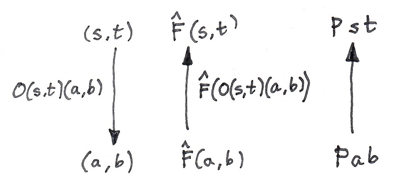
Let’s first analyze the definition of a presheaf $\hat F \in [\mathbf{Opt}^{op}, Set]$ . On objects, it maps pairs $(a, b)$ to sets $\hat F (a, b)$ .

On morphisms, it maps optics to functions (reversing the direction). Thus an optic:

$O(s, t) (a, b) = \int^{m \colon \mathbf M} C(s, m \triangleright a) \times C(m \triangleright b, t)$

is mapped to a function:

$\hat F (O (s, t)(a, b)) \colon \hat F (a, b) \to \hat F (s, t)$ .

The plan is to construct two mappings: from presheaves to Tambara modules and another from Tambara modules to presheaves. They have to be defined on (pairs of) objects as well as on morphisms. I will first sketch the proof using category theory and then translate it, step by step, to Haskell.

From presheaf to Tambara

On objects, given a presheaf $\hat F$ , we define a profunctor:

$P a b = \hat F (a, b)$

We know that it’s a profunctor because, given a pair of morphisms:

$h \colon a' \to a$
$h' \colon b \to b'$

we can construct a mapping:

$\hat F(a, b) \to \hat F (a', b')$

We do this by lifting an optic of the type:

$\int^m C(a', m \triangleright a) \times C(m \triangleright b, b')$

This optic can be instantiated by injecting $(1, \lambda^{-1}_a \circ h, h' \circ \lambda_b)$ into the coend.

The tricky part is to equip $P$ with the Tambara structure:

$\lambda_{ m, a b} \colon P a b \to P (m \triangleright a)( m \triangleright b)$

In this case, we want to implement:

$\lambda_{ m, a b} \colon \hat F (a, b) \to \hat F (m \triangleright a, m \triangleright b)$

We’ll do this by lifting a carefuly chosen optic of the type:

$O (m \triangleright a, a) (m \triangleright b, b)$

This optic is given by the following coend:

$\int^n C(m \triangleright a, n \triangleright a) \times C(n \triangleright b, m \triangleright b)$

We instantiate it by injecting the triple $(m, id_{m \triangleright a}, id_{m \triangleright b})$ into the coend.

On morphisms, we want to map an optic to an element of the hom-set $Set (P a b, P s t)$ . This mapping itself is an element of a bigger hom-set:

$Set \big( \int^m C(s, m \triangleright a) \times C(m \triangleright b, t), Set (P a b, P s t) \big)$

Using the co-continuity of the hom-set, we replace the mapping out of a coend with the end:

$\int_m Set \big( C(s, m \triangleright a) \times C(m \triangleright b, t), Set (P a b, P s t) \big)$

We have at our disposal a pair of morphisms:

$l \colon s \to m \triangleright a$
$r \colon m \triangleright b \to t$

which, together with the Tambara structure, give us the desired mapping:

$P a b \xrightarrow{\lambda m, a b} P (m \triangleright a)( m \triangleright b) \xrightarrow{P\, l\, r} P s t$

From Tambara to presheaf

On objects, given a Tambara module $P$ , we define a presheaf :

$\hat F a b = P a b$

On morphisms, we have to map a function on Tambara modules $P a b \to P s t$ to an optic. To do that, we need to come up with a specific Tambara module to feed it to this function. Since we want to produce an optic, it makes sense that we feed it an optic. The question is: Are optics Tambara modules?

An optic $O (s, t) (a, b)$ is a profunctor in each pair of arguments. Let’s see if we can come up with a Tambara structure in $(s, t)$ while keeping the pair $(a, b)$ constant. Given:

$\int^{m'} (C(s, m' \triangleright a) \times C(m' \triangleright b, t)$

We want to produce:

$\int^{m'} (C(m \triangleright s, m' \triangleright a) \times C(m' \triangleright b, m \triangleright t)$ .

We have at our disposal a pair of morphisms:

$l \colon s \to m' \triangleright a$
$r \colon m' \triangleright b \to t$

We know that simple hom-sets are Tambara modules, so we can apply the Tambara structure to both morphism:

$\lambda_{m, s, m' \triangleright a} \, l \colon m \triangleright s \to m \triangleright m' \triangleright a$
$\lambda_{m, m' \triangleright b} \, r \colon m \triangleright m' \triangleright b \to m \triangleright t$

After re-associating the iterated actions we inject the triple that consist of $m \otimes m'$ and the two resulting morphisms into our target coend.

Profunctor representation of optics

Since presheaves on $\mathbf{Opt}$ are Tambara modules, we can use the Tannakian reconstruction to represent a hom set in $\mathbf{Opt}$ as an end over Tambara modules:

$\int^{m \colon \mathbf M} C(s, m \triangleright a) \times C(m \triangleright b, t) \cong \int_{P \colon \mathbf{Tamb}} Set (P a b, P s t)$

This is the general form of the profunctor representation of optics that works for any monoidal action.

Haskell implementation

In Haskell, we can encode general optics (morphisms in $\mathbf{Opt}$ ) as:

			
data Opt ten act1 act2 s t a b = 
  forall m. (Actegory ten act1, Actegory ten act2) 
    => Opt (s -> m `act1` a) (m `act2` b -> t)

Notice that it’s okay to use two different actions (in fact, one can use two different categories). The corresponding Tambara modules are defined as:

			
class (Actegory ten act1, Actegory ten act2, Profunctor p) 
  => Tambara ten act1 act2 p where
    leftAct :: p a b -> p (m `act1` a) (m `act2` b)

The profunctor representation of these optics is given by a polymorphic function type:

			
type TamRep ten act1 act2 s t a b = 
    forall p . (Tambara ten act1 act2 p) => p a b -> p s t

Such functions can be composed (optics, zoomed in) using simple function composition.

Proof of equivalence

To prove the equivalence of the two representation, we need some additional definitions.

Here’s the unit optic that uses the unitors:

			
unitOpt :: (Actegory ten act1, Actegory ten act2) 
  => Opt ten act1 act2 a b a b
unitOpt = Opt unit' unit

Since we are working with the oposite category, we define the flipped version of optics:

			
data FlipOpt ten act1 act2 a b s t 
   = FlipOpt (Opt ten act1 act2 s t a b)

FlipOpt is an instance of Tambara:

			
instance (Actegory ten act1, Actegory ten act2) 
  => Tambara ten act1 act2 (FlipOpt ten act1 act2 a b) where
    leftAct (FlipOpt (Opt l r)) = FlipOpt (Opt l' r') 
      -- take advantage of the Tambara structure on hom-sets
      -- l :: s -> m a, l' :: n s -> n m a
      -- r :: m b -> t, r' :: n m b -> n t
      where l' = assoc' . leftAct @ten @act1 @act1 @(->) l
            r' =          leftAct @ten @act2 @act2 @(->) r . assoc
  

		

I made the use of the Tambara action on hom-functors explicit through type annotations.

Here’s the mapping from optics to the Tambara representation:

			
toProRep :: (Actegory ten act1, Actegory ten act2) => 
  Opt ten act1 act2 s t a b -> TamRep ten act1 act2 s t a b
toProRep (Opt s_ma mb_t) pab = dimap s_ma mb_t (leftAct pab)

The opposite mapping uses the flipped unit optics. This is why we needed the proof that flipped optic is a Tambara module. As such, we can pass it to our function that is polymorphic in Tambara modules:

			
fromProRep ::  (Actegory ten act1, Actegory ten act2) => 
  TamRep ten act1 act2 s t a b -> Opt ten act1 act2 s t a b
fromProRep pab_pst = opt
  where FlipOpt opt = pab_pst (FlipOpt unitOpt)

Examples

By plugging in different monoidal categories and their actions, we can immediately generate Tambara representations for a variety of optics.

We can use the Tambara encoding for the lens:

			
type Lens s t a b = forall p . 
  Tambara (,) (,) (,) p => p a b -> p s t

Here’s the example of a prism:

			
data Prism s t a b = forall m .
    Prism (s -> Either m a) (Either m b -> t)

and its Tambara representation:

			
type Prism' s t a b = forall p . 
  Tambara Either Either Either p => p a b -> p s t

Haskell code for this post is available here.

July 11, 2026

Tambara Equipment

Posted by Bartosz Milewski under Category Theory, Double category | Tags: Category Theory, Double Categories, Optics, Proarrow Equipment, Profunctors, Tambara Modules |
[2] Comments

I was originally attracted to category theory when trying to understand Haskell optics. I was puzzled by the van Laarhoven’s functor representations and Kmett’s use of Tambara modules. By playing Tetris with the Yoneda lemma I was able to make some progress, attacking more and more esoteric topics. With a group of researcher and students at the Oxford Adjoint School in Applied Category Theory we cracked the problem of traversal optics and published a paper summarizing the advances in profunctor optics.

Optics sit at an intersection of monoidal actions and Tambara modules. There is a duality between optics and Tambara representations. It is related to what mathematicians call Tannakian reconstruction, when an algebraic object is recovered from the totality of its representations.

No wonder then that a recent article by Mateusz Stroiński, Module categories, internal bimodules and Tambara modules, piqued my interest. It turns out that Tambara modules can be thought of as horizontal arrows in a double category, which is also a proarrow equipment. I will try to sketch the contents of this paper and illustrate it using Haskell code.

The slogan is that Tambara modules are to monoidal functors as profunctors are to functors.

The main advantage of the double-categorical setting for Tambara modules is that it works out of the box for enriched categories.

Monoidal functors redux

For simplicity, I’ll be using a simplified version of a strict monoidal functor, which omits the object constraint from the definition of a monoidal category:

			
class (Actegory ten act1, Actegory ten act2, Functor f) =>
  MonFunctor ten act1 act2 f where
    alpha  :: m `act2` f a -> f (m `act1` a)
    alpha' :: f (m `act1` a) -> m `act2` f a

Here, alpha' is the inverse of alpha.

Monoidal functors compose:

			
newtype MonFunCompose f g a = 
  MonFunCompose { getMonFunCompose :: f (g a) }

and the composition is again a monoidal functor:

			
instance ( Actegory ten act1
         , Actegory ten act2
         , Actegory ten act3
         , MonFunctor ten act2 act3 f
         , MonFunctor ten act1 act2 g) 
        => MonFunctor ten act1 act3 (MonFunCompose f g)
  where
    alpha mfga = 
        let m3fga' = second getMonFunCompose mfga
            fmga = alpha @ten @act2 @act3 m3fga'
            fgma = fmap (alpha @ten @act1 @act2) fmga
        in MonFunCompose fgma
    alpha' (MonFunCompose fgma) = 
        let fmga = fmap (alpha' @ten @act1 @act2) fgma
            mfga = alpha'  @ten @act2 @act3 fmga 
        in  second MonFunCompose mfga
  

		

Notice the use of type application to help the Haskell type checker.

Tambara modules

A Tambara module is a profunctor that is compatible with the action of a monoidal category. If you interpret a profunctor as a proof-relevant relation, a Tambara module has the property that, whenever two objects are related, they remain related when you “multiply” them by the same object $m$ . Multiplication in this case means the action of a monoidal category $\mathbf M$ . In other words, a Tambara module is a profunctor $J \colon A^{op} \times B \to \mathbf{Set}$ equipped with the transformation:

$\lambda_{m a b} \colon J a b \to J (m \triangleright_1 a) (m \triangleright_2 b)$

that is natural in $a$ and $b$ , and dinatural in $m$ . The action interacts nicely with the monoidal structure:

$\lambda_{(m \otimes n) a b} = \lambda_{m (n \triangleright a) (n \triangleright b)} \circ \lambda_{n a b}$

$\lambda_{1 a b} = id$

(modulo some associators and unitors).

We can illustrate this in Haskell as a typeclass:

			
class (Actegory ten act, Profunctor j) 
  => Tambara ten act j where
    leftAct :: j a b -> j (m `act` a) (m `act` b)

I chose to concentrate on the left action of the actegory, but it’s easy to define the right action, or both. For simplicity, I’m using the same action for both arguments. In full generality, we would have two separate actegories.

The simplest example of a Tambara module is the hom-functor:

			
instance (Actegory ten act) => Tambara ten act (->) where
    leftAct :: Actegory ten act => (a -> b) -> m `act` a -> m `act` b
    leftAct = second

Here I used the bifunctoriality of the action.

Tambara modules form a category, in which action-preserving natural transformations act as morphisms.

The usual profunctor composition using coends also works on Tambara modules.

			
data TamCompose p q d c where
  TamCompose :: p x c -> q d x -> TamCompose p q d c

The result of composition is again a Tambara module:

			
instance (Tambara ten act p, Tambara ten act q) 
  => Tambara ten act (TamCompose p q) where
    leftAct :: (Tambara ten act p, Tambara ten act q) =>
        TamCompose p q a b -> TamCompose p q (m `act` a) (m `act` b)
    leftAct (TamCompose pxc qdx) 
      = TamCompose (leftAct pxc) (leftAct qdx)
    

		

Taken together, we have a bicategory $\mathbf{Tam}$ , where actegories are 0-cells, Tambara modules with coend composition are 1-cells, and natural transformations between them are 2-cells.

Moreover, endo-Tambara modules, that is Tambara modules that operate within a single category, form a monoidal bicategory, with profunctor composition acting as a tensor product and a hom-functor acting as a unit.

Tambara Equipment

We have previously studied a double category $\mathbb{P}rof$ in which categories are 0-cells, profunctors are horizontal arrows, functors are vertical arrows, and natural transformations form 2-cells. This double category happens to be a proarrow equipment, which relates functors to representable profunctors in a specific way.

It turns out that there is an analogous construction with actegories as 0-cells, Tambara modules as horizontal 1-cells, and monoidal functors as vertical 1-cells. To form 2-cells, we first have to be able to lift (or restrict) a Tambara module along a pair of monoidal functors. We define a lifting of $J$ as the profunctor:

$\langle a, c \rangle \mapsto J(f a)(g c)$

or, using placeholders, $J(f -) (g =)$ . In Haskell this is:

newtype Lift f g j a c = Lift (j (f a) (g c))

The lifting of a Tambara module is again a Tambara module with the structure map defined as a composition:

$J (f a) (g c) \xrightarrow{\lambda_{m (f a) (g c)}} J (m \triangleright_2 f a) (m \triangleright_2 g c) \xrightarrow {J \alpha^{-1} \alpha} J (f (m \triangleright_1 a)) (g (m \triangleright_1 c))$

The second arrow lifts the (invertible) monoidal functor structure map to $J$ :

$\alpha \colon m \triangleright_2 g c \to g (m \triangleright_1 c)$

Here’s the same thing in Haskell:

			
instance ( Actegory ten act1
         , Actegory ten act2
         , MonFunctor ten act1 act2 f
         , MonFunctor ten act1 act2 g
         , Tambara ten act2 j) 
    => Tambara ten act1 (Lift f g j) where
    leftAct (Lift j) = Lift $ dimap alpha' alpha $ leftAct @ten @act2 j
    

		

I used type applications to select the correct left action corresponding to act2.

A 2-cell is then a natural transformation from $H$ to the lifting of $J$ .

Or, in Haskell:

type Cell f g h j = forall a c . h a c -> j (f a) (g c)

The companion and the conjoint are representable profunctors, that are automatically Tambara modules as long as f is a monoidal functor (the Identity functor is trivially monoidal):

			
type Companion f d c = Lift f Identity (->)
type Conjoint f d c  = Lift Identity f (->)

The unit and counit cells for the companion and the conjoint are reasonably easy to define (see the linked code).

Free Tambara and Optics

There is an obvious forgetful functor from $\mathbf{Tamb}$ to $\mathbf{Prof}$ (it forgets the action). This functor has a left adjoint. For any profunctor $J$ , it produces a free Tambara module given by the following coend:

$(\Phi J) \, s t = \int^m \int^{x y} C(s, m \triangleright x) \times J x y \times C(m \triangleright y, t)$

In Haskell, we model it as an existential data type:

			
data FreeTamb ten act j s t = 
  forall m x y. (MonoidalCategory ten, Actegory ten act) 
  => FreeTamb (s -> m `act` x) (j x y) (m `act` y -> t)

The result is indeed a Tambara module:

			
instance (Actegory ten act, MonoidalCategory ten, Profunctor j) 
  => Tambara ten act (FreeTamb ten act j) where
    -- na -> (nm)c, jcd, (nm)d -> nb
    leftAct (FreeTamb a_mc jcd md_b) = FreeTamb f jcd g
      where
        --f :: n `act` a -> (n `ten` m) `act` c
        f  na = assoc' $ second a_mc na
        --g :: (n `ten` m) `act` d -> n `act` b
        g nm_d= second md_b $ assoc nm_d
  

		

It so happens that optics can be defined as a free Tambara module acting on a representable profunctor $\Theta_{a b} x y = C(x, a) \times C(b, y)$ . Indeed, applying the Yoneda reduction, we get:

$O\, s t a b = \int^{m} C(s, m \triangleright a) \times C(m \triangleright b, t)$

In Haskell

data Rep a b x y = Rep (x -> a) (b -> y)

giving us:

type Optic ten s t a b = FreeTamb ten (Rep a b) s t

which, by Yoneda reduction, is isomorphic to:

			
data Optic ten act s t a b = forall m.
    Optic (s -> m `act` a) (m `act` b -> t)

Internalizing monoidal actions

A monoidal action, seen as a functor $\mathbf M \to [C, C]$ , can be internalized in $M$ if it has a right adjoint:

$C(m \triangleright a, t) \cong \mathbf M (m, \{a, t \} )$

If you think of the action as “multiplication,” the adjunction is reminiscent of currying, and the right adjoint plays to role on the “internal hom.”

In Haskell, we define a typeclass:

			
class (Actegory ten act, MonoidalCategory ten, Profunctor hom) 
  => IntHom ten act hom | hom -> act where
    icurry   :: (m `act` a -> b) -> (m -> hom a b)
    iuncurry :: (m -> hom a b)   -> (m `act` a -> b)

We can use this adjunction to simplify multiplicative optics:

$\int^{m} C(s, m \triangleright a) \times C(m \triangleright b, t) \cong \int^{m} C(s, m \triangleright a) \times \mathbf M (m, \{b, t \})$

Using the Yoneda reduction (a.k.a, “integrating” over $m$ ), this is equivalent to:

$O \, s t a b \cong C(s, \{b, t \} \triangleright a )$

With additive optics, we use the right adjoint to coproduct to produce hom-sets in a product category.

Both tricks are used in simplifying traversals, which are optics generated by polynomial functors:

$\int^{c \colon [\mathbb N , Set]} C(s, \sum_n c_n \times a^n) \times C (\sum_m c_m \times b^m, t)$

Here, $c$ is a natural-number-indexed family of objects with a monoidal structure given by convolution; and $a^n$ and $b^n$ are powers.

We first use the coproduct adjunction:

$C (\sum_m c_m \times b^m, t) \cong \prod_m C(c_m \times b^m, t)$

and follow it by the currying adjunction. We get the formula for a traversal:

$T \, s t a b \cong Set(s, \sum_n Set(b^n, t) \times a^n)$

The result can be illustrated in Haskell by replacing powers with lists:

type Traversal s t a b = s -> ([b] -> t, [a])

Internal monoid

The endo-hom $\{a, a\}$ is automatically a monoid in $\mathbf M$ . Indeed, we can define monoid multiplication as:

$\mathbf M(\{a, a\} \otimes \{a, a\}, \{a, a\}) \cong C\big((\{a, a\} \otimes \{a, a\}) \triangleright a, a\big)$

The right hand side can be implemented as a double application of the counit of the adjunction:

$\epsilon_{a a} = \{a, a\} \triangleright a \to a$

In Haskell, we first define a monoid internal to a monoidal category:

			
class (MonoidalCategory ten) => IMonoid ten m where
    imempty  :: Unit ten -> m
    imappend :: m `ten` m -> m

and show that hom a a is an instance of it:

			
instance (Actegory ten act, MonoidalCategory ten, IntHom ten act hom)  
  => IMonoid ten (hom a a) where
    imempty = icurry unit
    -- imappend :: (hom a a) `ten` (hom a a) -> hom a a
    imappend = icurry (eval . second eval . assoc)

where counit of the adjunction is the eval function:

			
eval :: (Actegory ten act, MonoidalCategory ten, IntHom ten act hom) 
  => hom a b `act` a -> b
eval = iuncurry id

Haskell code for this blog post is available here.

March 24, 2024

Neural Networks, Pre-lenses, and Triple Tambara Modules, Part II

Posted by Bartosz Milewski under Category Theory, Lens, Neural Networks, Programming | Tags: AI, Category Theory, Lens, Neural Networks, Optics, Profunctors, Tambara Modules |
1 Comment

I will now provide the categorical foundation of the Haskell implementation from the previous post. A PDF version that contains both parts is also available.

The Para Construction

There’s been a lot of interest in categorical foundations of deep learning. The basic idea is that of a parametric category, in which morphisms are parameterized by objects from a monoidal category $\mathcal P$ :

Screenshot 2024-03-24 at 15.00.20
Here, $p$ is an object of $\mathcal P$ .

When two such morphisms are composed, the result is parameterized by the tensor product of the parameters.

Screenshot 2024-03-24 at 15.00.34

An identity morphism is parameterized by the monoidal unit $I$ .

If the monoidal category $\mathcal P$ is not strict, the parametric composition and identity laws are not strict either. They are satisfied up to associators and unitors of $\mathcal P$ . A category with lax composition and identity laws is called a bicategory. The 2-cells in a parametric bicategory are called reparameterizations.

Of particular interest are parameterized bicategories that are built on top of actegories. An actegory $\mathcal C$ is a category in which we define an action of a monoidal category $\mathcal P$ :

$\bullet \colon \mathcal P \times \mathcal C \to C$

satisfying some obvious coherency conditions (unit and composition):

$I \bullet c \cong c$

$p \bullet (q \bullet c) \cong (p \otimes q) \bullet c$

There are two basic constructions of a parametric category on top of an actegory called $\mathbf{Para}$ and $\mathbf{coPara}$ . The first constructs parametric morphisms from $a$ to $b$ as $f_p = p \bullet a \to b$ , and the second as $g_p = a \to p \bullet b$ .

Parametric Optics

The $\mathbf{Para}$ construction can be extended to optics, where we’re dealing with pairs of objects from the underlying category (or categories, in the case of mixed optics). The parameterized optic is defined as the following coend:

$O \langle a, da \rangle \langle p, dp \rangle \langle s, ds \rangle = \int^{m} \mathcal C (p \bullet s, m \bullet a) \times \mathcal C (m \bullet da, dp \bullet ds)$

where the residues $m$ are objects of some monoidal category $\mathcal M$ , and the parameters $\langle p, dp \rangle$ come from another monoidal category $\mathcal P$ .

In Haskell, this is exactly the existential lens:

data ExLens a da p dp s ds = 
  forall m . ExLens ((p, s)  -> (m, a))  
                    ((m, da) -> (dp, ds))

There is, however, a more general bicategory of pre-optics, which underlies existential optics. In it, both the parameters and the residues are treated symmetrically.

The PreLens Bicategory

Pre-optics break the feedback loop in which the residues from the forward pass are fed back to the backward pass. We get the following formula:

$\begin{aligned}O & \langle a, da \rangle \langle m, dm \rangle \langle p, dp \rangle \langle s, ds \rangle = \\ &\mathcal C (p \bullet s, m \bullet a) \times \mathcal C (dm \bullet da, dp \bullet ds) \end{aligned}$

We interpret this as a hom-set from a pair of objects $\langle s, ds \rangle$ in $\mathcal C^{op} \times C$ to the pair of objects $\langle a, da \rangle$ also in $\mathcal C^{op} \times C$ , parameterized by a pair $\langle m, dm \rangle$ in $\mathcal M \times \mathcal M^{op}$ and a pair $\langle p, dp \rangle$ from $\mathcal P^{op} \times \mathcal P$ .

To simplify notation, I’ll use the bold $\mathbf C$ for the category $\mathcal C^{op} \times \mathcal C$ , and bold letters for pairs of objects and (twisted) pairs of morphisms. For instance, $\bold f \colon \bold a \to \bold b$ is a member of the hom-set $\mathbf C (\bold a, \bold b)$ represented by a pair $\langle f \colon a' \to a, g \colon b \to b' \rangle$ .

Similarly, I’ll use the notation $\bold m \bullet \bold a$ to denote the monoidal action of $\mathcal M^{op} \times \mathcal M$ on $\mathcal C^{op} \times \mathcal C$ :

$\langle m, dm \rangle \bullet \langle a, da \rangle = \langle m \bullet a, dm \bullet da \rangle$

and the analogous action of $\mathcal P^{op} \times \mathcal P$ .

In this notation, the pre-optic can be simply written as:

$O\; \bold a\, \bold m\, \bold p\, \bold s = \bold C (\bold m \bullet \bold a, \bold p \bullet \bold b)$

and an individual morphism as a triple:

$(\bold m, \bold p, \bold f \colon \bold m \bullet \bold a \to \bold p \bullet \bold b)$

Pre-optics form hom-sets in the $\mathbf{PreLens}$ bicategory. The composition is a mapping:

$\mathbf C (\bold m \bullet \bold b, \bold p \bullet \bold c) \times \mathbf C (\bold n \bullet \bold a, \bold q \bullet \bold b) \to \mathbf C (\bold (\bold m \otimes \bold n) \bullet \bold a, (\bold q \otimes \bold p) \bullet \bold c)$

Indeed, since both monoidal actions are functorial, we can lift the first morphism by $(\bold q \bullet -)$ and the second by $(\bold m \bullet -)$ :

$\mathbf C (\bold m \bullet \bold b, \bold p \bullet \bold c) \times \mathbf C (\bold n \bullet \bold a, \bold q \bullet \bold b) \xrightarrow{(\bold q \bullet) \times (\bold m \bullet)}$

$\mathbf C (\bold q \bullet \bold m \bullet \bold b, \bold q \bullet \bold p \bullet \bold c) \times \mathbf C (\bold m \bullet \bold n \bullet \bold a,\bold m \bullet \bold q \bullet \bold b)$

We can compose these hom-sets in $\mathbf C$ , as long as the two monoidal actions commute, that is, if we have:

$\bold q \bullet \bold m \bullet \bold b \to \bold m \bullet \bold q \bullet \bold b$

for all $\bold q$ , $\bold m$ , and $\bold b$ .
The identity morphism is a triple:

$(\bold 1, \bold 1, \bold{id} )$

parameterized by the unit objects in the monoidal categories $\mathbf M$ and $\mathbf P$ . Associativity and identity laws are satisfied modulo the associators and the unitors.

If the underlying category $\mathcal C$ is monoidal, the $\mathbf{PreOp}$ bicategory is also monoidal, with the obvious point-wise parallel composition of pre-optics.

Triple Tambara Modules

A triple Tambara module is a functor:

$T \colon \mathbf M^{op} \times \mathbf P \times \mathbf C \to \mathbf{Set}$

equipped with two families of natural transformations:

$\alpha \colon T \, \bold m \, \bold p \, \bold a \to T \, (\bold n \otimes \bold m) \, \bold p \, (\bold n \bullet a)$

$\beta \colon T \, \bold m \, \bold p \, (\bold r \bullet \bold a) \to T \, \bold m \, (\bold p \otimes \bold r) \, \bold a$

and some coherence conditions. For instance, the two paths from $T \, \bold m \, \bold p\, (\bold r \bullet \bold a)$ to $T \, (\bold n \otimes \bold m)\, (\bold p \otimes \bold r) \, (\bold n \bullet \bold a)$ must give the same result.

One can also define natural transformations between such functors that preserve the two structures, and define a bicategory of triple Tambara modules $\mathbf{TriTamb}$ .

As a special case, if we chose the category $\mathcal P$ to be the trivial one-object monoidal category, we get a version of (double-) Tambara modules. If we then take the coend, $P \langle a, b \rangle = \int^m T \langle m, m\rangle \langle a, b \rangle$ , we get regular Tambara modules.

Pre-optics themselves are an example of a triple Tambara representation. Indeed, for any fixed $\bold a$ , we can define a mapping $\alpha$ from the triple:

$(\bold m, \bold p, \bold f \colon \bold m \bullet \bold a \to \bold p \bullet \bold b)$

to the triple:

$(\bold n \otimes \bold m, \bold p, \bold f' \colon (\bold n \otimes \bold m) \bullet \bold a \to \bold p \bullet (\bold n \bullet \bold b))$

by lifting of $\bold f$ by $(\bold n \bullet -)$ and rearranging the actions using their commutativity.
Similarly for $\beta$ , we map:

$(\bold m, \bold p, \bold f \colon \bold m \bullet \bold a \to \bold p \bullet (\bold r \bullet \bold b))$

to:

$(\bold m , (\bold p \otimes \bold r), \bold f' \colon \bold m \bullet \bold a \to (\bold p \otimes \bold r) \bullet \bold b)$

Tambara Representation

The main result is that morphisms in $\mathbf {PreOp}$ can be expressed using triple Tambara modules. An optic:

$(\bold m, \bold p, \bold f \colon \bold m \bullet \bold a \to \bold p \bullet \bold b)$

is equivalent to a triple end:

$\int_{\bold r \colon \mathbf P} \int_{\bold n \colon \mathbf M} \int_{T \colon \mathbf{TriTamb}} \mathbf{Set} \big(T \, \bold n \, \bold r \, \bold a, T \, (\bold m \otimes \bold n) \, (\bold r \otimes \bold p) \, \bold b \big)$

Indeed, since pre-optics are themselves triple Tambara modules, we can apply the polymorphic mapping of Tambara modules to the identity optic $(\bold 1, \bold 1, \bold{id} )$ and get an arbitrary pre-optic.

Conversely, given an optic:

$(\bold m, \bold p, \bold f \colon \bold m \bullet \bold a \to \bold p \bullet \bold b)$

we can construct the polymorphic mapping of triple Tambara modules:

$\begin{aligned} & T \, \bold n \, \bold r \, \bold a \xrightarrow{\alpha} T \, (\bold m \otimes \bold n) \, \bold r \, (\bold m \bullet \bold a) \xrightarrow{T \, \bold f} T \, (\bold m \otimes \bold n) \, \bold r \, (\bold p \bullet \bold b) \xrightarrow{\beta} \\ & T \, (\bold m \otimes \bold n) \, (\bold r \otimes \bold p) \, \bold b \end{aligned}$

Bibliography

Brendan Fong, Michael Johnson, Lenses and Learners,
Brendan Fong, David Spivak, Rémy Tuyéras, Backprop as Functor: A compositional perspective on supervised learning, 34th Annual ACM/IEEE Symposium on Logic in Computer Science (LICS) 2019, pp. 1-13, 2019.
G.S.H. Cruttwell, Bruno Gavranović, Neil Ghani, Paul Wilson, Fabio Zanasi, Categorical Foundations of Gradient-Based Learning
Bruno Gavranović, Compositional Deep Learning
Bruno Gavranović, Fundamental Components of Deep Learning, PhD Thesis. 2024

March 22, 2024

Neural Networks, Pre-Lenses, and Triple Tambara Modules

Posted by Bartosz Milewski under Programming | Tags: AI, artificial-intelligence, deep-learning, Lens, machine-learning, Neural Networks, Optics, Profunctors, Tambara Modules |
1 Comment

Introduction

Neural networks are an example of composable systems, so it’s no surprise that they can be modeled in category theory, which is the ultimate science of composition. Moreover, the categorical ideas behind neural networks can be immediately implemented and tested in a programming language. In this post I will present the Haskell implementation of parametric lenses, generalize them to pre-lenses and introduce their profunctor representation. Using the profunctor representation I will build a working multi-layer perceptron.

In the second part of this post I will introduce the bicategory $\mathbf{PreLens}$ of pre-lenses and the bicategory of triple Tambara profunctors and show how they related to pre-lenses.

Complete Haskell implementation is available on gitHub, where you can also find the PDF version of this post, complete with the categorical picture.

Haskell Implementation

Every component of a neural network can be thought of as a system that transform input to output, and whose action depends on some parameters. In the language of neural networsks, this is called the forward pass. It takes a bunch of parameters p, combines it with the input s, and produces the output a. It can be described by a Haskell function:

fwd :: (p, s) -> a

But the real power of neural networks is in their ability to learn from mistakes. If we don’t like the output of the network, we can nudge it towards a better solution. If we want to nudge the output by some da, what change dp to the parameters should we make? The backward pass partitions the blame for the perceived error in direct proportion to the impact each parameter had on the result.

Because neural networks are composed of layers of neurons, each with their own sets or parameters, we might also ask the question: What change ds to this layer’s inputs (which are the outputs of the previous layer) should we make to improve the result? We could then back-propagate this information to the previous layer and let it adjust its own parameters. The backward pass can be described by another Haskell function:

bwd :: (p, s, da) -> (dp, ds)

The combination of these two functions forms a parametric lens:

data PLens a da p dp s ds = 
  PLens { fwd :: (p, s) -> a
        , bwd :: (p, s, da) -> (dp, ds) }

In this representation it’s not immediately obvious how to compose parametric lenses, so I’m going to present a variety of other representations that may be more convenient in some applications.

Existential Parametric Lens

Notice that the backward pass re-uses the arguments (p, s) of the forward pass. Although some information from the forward pass is needed for the backward pass, it’s not always clear that all of it is required. It makes more sense for the forward pass to produce some kind of a care package to be delivered to the backward pass. In the simplest case, this package would just be the pair (p, s). But from the perspective of the user of the lens, the exact type of this package is an internal implementation detail, so we might as well hide it as an existential type m. We thus arrive at a more symmetric representation:

data ExLens a da p dp s ds = 
  forall m . ExLens ((p, s)  -> (m, a))  
                    ((m, da) -> (dp, ds))

The type m is often called the residue of the lens.

These existential lenses can be composed in series. The result of the composition is parameterized by the product (a tuple) of the original parameters. We’ll see it more clearly in the next section.

But since the product of types is associative only up to isomorphism, the composition of parametric lenses is associative only up to isomorphism.

There is also an identity lens:

identityLens :: ExLens a da () () a da
identityLens = ExLens id id

but, again, the categorical identity laws are satisfied only up to isomorphism. This is why parametric lenses cannot be interpreted as hom-sets in a traditional category. Instead they are part of a bicategory that arises from the $\mathbf{Para}$ construction.

Pre-Lenses

Notice that there is still an asymmetry in the treatment of the parameters and the residues. The parameters are accumulated (tupled) during composition, while the residues are traced over (categorically, an existential type is described by a coend, which is a generalized trace). There is no reason why we shouldn’t accumulate the residues during composition and postpone the taking of the trace untill the very end.

We thus arrive at a fully symmetrical definition of a pre-lens:

data PreLens a da m dm p dp s ds =
  PreLens ((p, s)   -> (m, a))
          ((dm, da) -> (dp, ds))

We now have two separate types: m describing the residue, and dm describing the change of the residue.

Screenshot 2024-03-22 at 12.19.58

If all we need at the end is to trace over the residues, we’ll identify the two types.

Notice that the role of parameters and residues is reversed between the forward and the backward pass. The forward pass, given the parameters and the input, produces the output plus the residue. The backward pass answers the question: How should we nudge the parameters and the inputs (dp, ds) if we want the residues and the outputs to change by (dm, da). In neural networks this will be calculated using gradient descent.

The composition of pre-lenses accumulates both the parameters and the residues into tuples:

preCompose ::
    PreLens a' da' m dm p dp s ds -> 
    PreLens a da n dn q dq a' da' ->
    PreLens a da (m, n) (dm, dn) (q, p) (dq, dp) s ds
preCompose (PreLens f1 g1) (PreLens f2 g2) = PreLens f3 g3
  where
    f3 = unAssoc . second f2 . assoc . first sym . 
         unAssoc . second f1 . assoc
    g3 = unAssoc . second g1 . assoc . first sym . 
         unAssoc . second g2 . assoc

We use associators and symmetrizers to rearrange various tuples. Notice the separation of forward and backward passes. In particular, the backward pass of the composite lens depends only on backward passes of the composed lenses.

There is also an identity pre-lens:

idPreLens :: PreLens a da () () () () a da
idPreLens = PreLens id id

Pre-lenses thus form a bicategory that combines the $\mathbf{Para}$ and the $\mathbf{coPara}$ constructions in one.

There is also a monoidal structure in this category induced by parallel composition. In parallel composition we tuple the respective inputs and outputs, as well as the parameters and residues, both in the forward and the backward passes.

The existential lens can be obtained from the pre-lens at any time by tracing over the residues:

data ExLens a da p dp s ds = 
  forall m. ExLens (PreLens a da m m p dp s ds)

Notice however that the tracing can be performed after we are done with all the (serial and parallel) compositions. In particular, we could dedicate one pipeline to perform forward passes, gathering both parameters and residues, and then send this data over to another pipeline that performs backward passes. The data is produced and consumed in the LIFO order.

Pre-Neuron

As an example, let’s implement the basic building block of neural networks, the neuron. In what follows, we’ll use the following type synonyms:

type D = Double
type V = [D]

A neuron can be decomposed into three mini-layers. The first layer is the linear transformation, which calculates the scalar product of the input vector and the vector of parameters:

$a = \sum_{i = 1}^n p_i \times s_i$

It also produces the residue which, in this case, consists of the tuple (V, V) of inputs and parameters:

fw :: (V, V) -> ((V, V), D)
fw (p, s) = ((s, p), sumN n $ zipWith (*) p s)

The backward pass has the general signature:

bw :: ((dm, da) -> (dp, ds))

Because we’re eventually going to trace over the residues, we’ll use the same type for dm as for m. And because we are going to do arithmetic over the parameters, we reuse the type of p for the delta dp. Thus the signature of the backward pass is:

bw :: ((V, V), D) -> (V, V)

In the backward pass we’ll encode the gradient descent. The steepest gradient direction and slope is given by the partial derivatives:

$\frac{\partial{ a}}{\partial p_i} = s_i$

$\frac{\partial{ a}}{\partial s_i} = p_i$

We multiply them by the desired change in the output da:

dp = fmap (da *) s
ds = fmap (da *) p

Here’s the resulting lens:

linearL :: Int -> PreLens D D (V, V) (V, V) V V V V
linearL n = PreLens fw bw
  where
    fw :: (V, V) -> ((V, V), D)
    fw (p, s) = ((s, p), sumN n $ zipWith (*) p s)
    bw :: ((V, V), D) -> (V, V)
    bw ((s, p), da) = (fmap (da *) s
                      ,fmap (da *) p)

The linear transformation is followed by a bias, which uses a single number as the parameter, and generates no residue:

biasL :: PreLens D D () () D D D D
biasL = PreLens fw bw 
  where 
    fw :: (D, D) -> ((), D)
    fw (p, s) = ((), p + s)
    -- da/dp = 1, da/ds = 1
    bw :: ((), D) -> (D, D)
    bw (_, da) = (da, da)

Finally, we implement the non-linear activation layer using the tanh function:

activL :: PreLens D D D D () () D D
activL = PreLens fw bw
  where
    fw (_, s) = (s, tanh s)
    -- da/ds = 1 + (tanh s)^2
    bw (s, da)= ((), da * (1 - (tanh s)^2))

A neuron with $m$ inputs is a composition of the three components, modulo some monoidal rearrangements:

neuronL :: Int -> 
    PreLens D D ((V, V), D) ((V, V), D) Para Para V V

neuronL mIn = PreLens f' b'
  where 
    PreLens f b = 
      preCompose (preCompose (linearL mIn) biasL) activL
    f' :: (Para, V) -> (((V, V), D), D)
    f' (Para bi wt, s) = let (((vv, ()), d), a) = 
        f (((), (bi, wt)), s)
                         in ((vv, d), a)
    b' :: (((V, V), D), D) -> (Para, V)
    b' ((vv, d), da) = let (((), (d', w')), ds) = 
        b (((vv, ()), d), da)
                       in (Para d' w', ds)

The parameters for the neuron can be conveniently packaged into one data structure:

data Para = Para { bias   :: D
                 , weight :: V }

mkPara (b, v) = Para b v
unPara p = (bias p, weight p)

Using parallel composition, we can create whole layers of neurons, and then use sequential composition to model multi-layer neural networks. The loss function that compares the actual output with the expected output can also be implemented as a lens. We’ll perform this construction later using the profunctor representation.

Tambara Modules

As a rule, all optics that have an existential representation also have some kind of profunctor representation. The advantage of profunctor representations is that they are functions, and they compose using function composition.

Lenses, in particular, have a representation using a special category of profunctors called Tambara modules. A vanilla Tambara module is a profunctor p equipped with a family of transformations. It can be implemented as a Haskell class:

class  Profunctor p => Tambara p where
  alpha :: forall a da m. p a da -> p (m, a) (m, da)

The vanilla lens is then represented by the following profunctor-polymorphic function:

type Lens a da s ds = forall p. Tambara p => p a da -> p s ds

A similar representation can be constructed for pre-lenses. A pre-lens, however, has additional dependency on parameters and residues, so the analog of a Tambara module must also be parameterized by those. We need, therefore, a more complex type constructor t that takes six arguments:

t m dm p dp s ds

This is supposed to be a profunctor in three pairs of arguments, s ds, p dp, and dm m. Pro-functoriality in the first two pairs is implemented as two functions, diampS and dimapP. The inverted order in dm m means that t is covariant in m and contravariant in dm, as seen in the unusual type signature of dimapM:

dimapM  :: (m -> m') -> (dm' -> dm) -> 
  t m dm p dp s ds -> t m' dm' p  dp  s  ds

To generalize Tambara modules we first observe that the pre-lens now has two independent residues, m and dm, and the two should transform separately. Also, the composition of pre-lenses accumulates (through tupling) both the residues and the parameters, so it makes sense to use the additional type arguments to TriProFunctor as accumulators. Thus the generalized Tambara module has two methods, one for accumulating residues, and one for accumulating parameters:

class TriProFunctor t => Trimbara t where
  alpha :: t m dm p dp s ds -> 
           t (m1, m) (dm1, dm) p dp (m1, s) (dm1, ds)
  beta  :: t m dm p dp (p1, s) (dp1, ds) -> 
           t m dm (p, p1) (dp, dp1) s ds

These generalized Tambara modules satisfy some coherency conditions.

One can also define natural transformations that are compatible with the new structures, so that Trimbara modules form a category.

The question arises: can this definition be satisfied by an actual non-trivial TriProFunctor? Fortunately, it turns out that a pre-lens itself is an example of a Trimbara module. Here’s the implementation of alpha for a PreLens:

alpha (PreLens fw bw) = PreLens fw' bw'
  where
    fw' (p, (n, s)) = let (m, a) = fw (p, s)
                      in ((n, m), a)
    bw' ((dn, dm), da) = let (dp, ds) = bw (dm, da)
                         in (dp, (dn, ds))

and this is beta:

beta (PreLens fw bw) = PreLens fw' bw'
  where
    fw' ((p, r), s) = let (m, a) = fw (p, (r, s))
                      in (m, a)
    bw' (dm, da) = let (dp, (dr, ds)) = bw (dm, da)
                   in ((dp, dr), ds)

This result will become important in the next section.

TriLens

Since Trimbara modules form a category, we can define a polymorphic function type (a categorical end) over Trimbara modules . This gives us the (tri-)profunctor representation for a pre-lens:

type TriLens a da m dm p dp s ds =
    forall t. Trimbara t => forall p1 dp1 m1 dm1. 
      t m1 dm1 p1 dp1 a da -> 
      t (m, m1) (dm, dm1) (p1, p) (dp1, dp) s ds

Indeed, given a pre-lens we can construct the requisite mapping of Trimbara modules simply by lifting the two functions (the forward and the backward pass) and sandwiching them between the two Tambara structure maps:

toTamb :: PreLens a da m dm p dp s ds -> 
    TriLens a da m dm p dp s ds
toTamb (PreLens fw bw) = beta . dimapS fw bw . alpha

Conversely, given a mapping between Trimbara modules, we can construct a pre-lens by applying it to the identity pre-lens (modulo some rearrangement of tuples using the monoidal right/left unit laws):

fromTamb :: TriLens a da m dm p dp s ds -> 
    PreLens a da m dm p dp s ds
fromTamb f = dimapM runit unRunit $  
             dimapP unLunit lunit $ 
             f idPreLens

The main advantage of the profunctor representation is that we can now compose two lenses using simple function composition; again, modulo some associators:

triCompose ::
    TriLens b db m dm p dp s ds -> 
    TriLens a da n dn q dq b db ->
    TriLens a da (m, n) (dm, dn) (q, p) (dq, dp) s ds
triCompose f g = dimapP unAssoc assoc . 
                 dimapM unAssoc assoc . 
                 f . g

Parallel composition of TriLenses is also relatively straightforward, although it involves a lot of bookkeeping (see the gitHub implementation).

Training a Neural Network

As a proof of concept, I have implemented and trained a simple 3-layer perceptron.

The starting point is the conversion of the individual components of the neuron from their pre-lens representation to the profunctor representation using toTamb. For instance:

linearT :: Int -> TriLens D D (V, V) (V, V) V V V V
linearT n = toTamb (linearL n)

We get a profunctor representation of a neuron by composing its three components:

neuronT :: Int -> 
  TriLens D D ((V, V), D) ((V, V), D) Para Para V V
neuronT mIn = 
  dimapP (second (unLunit . unPara)) 
         (second (mkPara . lunit)) .
  triCompose (dimapM (first runit) (first unRunit) .
  triCompose (linearT mIn) biasT) activT

With parallel composition of tri-lenses, we can build a layer of neurons of arbitrary width.

layer :: Int -> Int -> 
  TriLens V V [((V, V), D)] [((V, V), D)] [Para] [Para] V V
layer mIn nOut = 
  dimapP (second unRunit) (second runit) .
  dimapM (first lunit) (first unLunit) .
  triCompose (branch nOut) (vecLens nOut (neuronT mIn))

The result is again a tri-lens, and such tri-lenses can be composed in series to create a multi-layer perceptron.

makeMlp :: Int -> [Int] -> 
  TriLens V V -- output
          [[((V, V), D)]] [[((V, V), D)]] -- residues
          [[Para]] [[Para]] -- parameters
          V V -- input

Here, the first integer specifies the number of inputs of each neuron in the first layer. The list [Int] specifies the number of neurons in consecutive layers (which is also the number of inputs of each neuron in the following layer).

The training of a neural network is usually done by feeding it a batch of inputs together with a batch of expected outputs. This can be simply done by arranging multiple perceptrons in parallel and accumulating the parameters for the whole batch.

batchN :: (VSpace dp) => Int -> 
    TriLens  a da m dm p dp s ds -> 
    TriLens [a] [da] [m] [dm] p dp [s] [ds]

To make the accumulation possible, the parameters must form a vector space, hence the constraint VSpace dp.

The whole thing is then capped by a square-distance loss lens that is parameterized by the ground truth values:

lossL :: PreLens D D ([V], [V]) ([V], [V]) [V] [V] [V] [V]
lossL = PreLens fw bw 
  where
    fw (gTruth, s) = 
      ((gTruth, s), sqDist (concat s) (concat gTruth))
    bw ((gTruth, s), da) = (fmap (fmap negate) delta', delta')
      where
        delta' = fmap (fmap (da *)) (zipWith minus s gTruth)

In the next post I will present the categorical version of this construction.

February 7, 2024

Linear Lenses in Haskell

Posted by Bartosz Milewski under Programming | Tags: Category Theory, education, Functional Programming, hinduism, mathematics, Optics, Profunctors, Tambara Modules |
[3] Comments

I always believed that the main problems in designing a programming language were resource management and concurrency–and the two are related. If you can track ownership of resources, you can be sure that no synchronization is needed when there’s a single owner.

I’ve been evangelizing resource management for a long time, first in C++, and then in D (see Appendix 3). I was happy to see it implemented in Rust as ownership types, and I’m happy to see it coming to Haskell as linear types.

Haskell has essentially solved the concurrency and parallelism problems by channeling mutation to dedicated monads, but resource management has always been part of the awkward squad. The main advantage of linear types in Haskell, other than dealing with external resources, is to allow safe mutation and non-GC memory management. This could potentially lead to substantial performance gains.

This post is based on very informative discussions I had with Arnaud Spiwack, who explained to me the work he’d done on linear types and linear lenses, some of it never before documented.

The PDF version of this post together with complete Haskell code is available on GitHub.

Linear types

What is a linear function? The short answer is that a linear function $a \multimap b$ “consumes” its argument exactly once. This is not the whole truth, though, because we also have linear identity $id_a \colon a \multimap a$ , which ostensibly does not consume $a$ . The long answer is that a linear function consumes its argument exactly once if it itself is consumed exactly once, and its result is consumed exactly once.

What remains to define is what it means to be consumed. A function is consumed when it’s applied to its argument. A base value like Int or Char is consumed when it’s evaluated, and an algebraic data type is consumed when it’s pattern-matched and all its matched components are consumed.

For instance, to consume a linear pair (a, b), you pattern-match it and then consume both a and b. To consume Either a b, you pattern-match it and consume the matched component, either a or b, depending on which branch was taken.

As you can see, except for the base values, a linear argument is like a hot potato: you “consume” it by passing it to somebody else.

So where does the buck stop? This is where the magic happens: Every resource comes with a special primitive that gets rid of it. A file handle gets closed, memory gets deallocated, an array gets frozen, and Frodo throws the ring into the fires of Mount Doom.

To notify the type system that the resource has been destroyed, a linear function will return a value inside the special unrestricted type Ur. When this type is pattern-matched, the original resource is finally destroyed.

For instance, for linear arrays, one such primitive is toList:

$\mathit{toList} \colon \text{Array} \; a \multimap \text{Ur} \, [a]$

In Haskell, we annotate the linear arrows with multiplicity 1:

toList :: Array a %1-> Ur  [a]

Similarly, magic is used to create the resource in the first place. For arrays, this happens inside the primitive fromList.

$\mathit{fromList} \colon [a] \to (\text{Array} \; a \multimap \text{Ur} \; b) \multimap \text{Ur} \; b$

or using Haskell syntax:

fromList :: [a] -> (Array a %1-> Ur b) %1-> Ur b

The kind of resource management I advertised in C++ was scope based. A resource was encapsulated in a smart pointer that was automatically destroyed at scope exit.

With linear types, the role of the scope is played by a user-provided linear function; here, the continuation:

(Array a %1 -> Ur b)

The primitive fromList promises to consume this user-provided function exactly once and to return its unrestricted result. The client is obliged to consume the array exactly once (e.g., by calling toList). This obligation is encoded in the type of the continuation accepted by fromList.

Linear lens: The existential form

A lens abstracts the idea of focusing on a part of a larger data structure. It is used to access or modify its focus. An existential form of a lens consists of two functions: one splitting the source into the focus and the residue; and the other replacing the focus with a new value, and creating a new whole. We don’t care about the actual type of the residue so we keep it as an existential.

The way to think about a linear lens is to consider its source as a resource. The act of splitting it into a focus and a residue is destructive: it consumes its source to produce two new resources. It splits one hot potato s into two hot potatoes: the residue c and the focus a.

Conversely, the part that rebuilds the target t must consume both the residue c and the new focus b.

We end up with the following Haskell implementation:

data LinLensEx a b s t where
  LinLensEx :: (s %1-> (c, a)) -> 
               ((c, b) %1-> t) -> LinLensEx a b s t

A Haskell existential type corresponds to a categorical coend, so the above definition is equivalent to:

$L a b s t = \int^c (s \multimap c \otimes a)\times (c \otimes b \multimap t)$

I use the lollipop notation for the hom-set in a monoidal category with a tensor product $\otimes$ .

The important property of a monoidal category is that its tensor product doesn’t come with a pair of projections; and the unit object is not terminal. In particular, a morphism $s \multimap c \otimes a$ cannot be decomposed into a product of two morphisms $(s \multimap c) \times (s \multimap a)$ .

However, in a closed monoidal category we can curry a mapping out of a tensor product:

$c \otimes b \multimap t \cong c \multimap (b \multimap t)$

We can therefore rewrite the existential lens as:

$L a b s t \cong \int^c (s \multimap c \otimes a)\times (c \multimap (b \multimap t))$

and then apply the co-Yoneda lemma to get:

$s \multimap \big((b \multimap t) \otimes a\big)$

Unlike the case of a standard lens, this form cannot be separated into a get/set pair.

The intuition is that a linear lens lets you consume the object $s$ , but it leaves you with the obligation to consume both the setter $b \multimap t$ and the focus $a$ . You can’t just extract $a$ alone, because that would leave a gaping hole in your object. You have to plug it in with a new object $b$ , and that’s what the setter lets you do.

Here’s the Haskell translation of this formula (conventionally, with the pairs of arguments reversed):

type LinLens s t a b = s %1-> (b %1-> t, a)

The Yoneda shenanigans translate into a pair of Haskell functions. Notice that, just like in the co-Yoneda trick, the existential $c$ is replaced by the linear function $b \multimap t$ .

fromLinLens :: forall s t a b.
  LinLens s t a b -> LinLensEx a b s t
fromLinLens h = LinLensEx f g
  where
    f :: s %1-> (b %1-> t, a)
    f = h
    g :: (b %1-> t, b) %1-> t
    g (set, b) = set b

The inverse mapping is:

toLinLens :: LinLensEx a b s t -> LinLens s t a b
toLinLens (LinLensEx f g) s = 
  case f s of
    (c, a) -> (\b -> g (c, b), a)

Profunctor representation

Every optic comes with a profunctor representation and the linear lens is no exception. Categorically speaking, a profunctor is a functor from the product category $\mathcal C^{op} \times \mathcal C$ to $\mathbf{Set}$ . It maps pairs of object to sets, and pairs of morphisms to functions. Since we are in a monoidal category, the morphisms are linear functions, but the mappings between sets are regular functions (see Appendix 1). Thus the action of the profunctor $p$ on morphisms is a function:

$(a' \multimap a) \to (b \multimap b') \to p a b \to p a' b'$

In Haskell:

class Profunctor p where
  dimap :: (a' %1-> a) -> (b %1-> b') -> p a b -> p a' b'

A Tambara module (a.k.a., a strong profunctor) is a profunctor equipped with the following mapping:

$\alpha_{a b c} \colon p a b \to p (c \otimes a) (c \otimes b)$

natural in $a$ and $b$ , dintural in $c$ .
In Haskell, this translates to a polymorphic function:

class (Profunctor p) => Tambara p where
   alpha :: forall a b c. p a b -> p (c, a) (c, b)

The linear lens $L a b s t$ is itself a Tambara module, for fixed $a b$ . To show this, let’s construct a mapping:

$\alpha_{s t c} \colon L a b s t \to L a b (c \otimes s) (c \otimes t)$

Expanding the definition:

$\int^{c''} (s \multimap c'' \otimes a)\times (c'' \otimes b \multimap t) \to$
$\; \int^{c' } (c \otimes s \multimap c' \otimes a)\times (c' \otimes b \multimap c \otimes t)$

By cocontinuity of the hom-set in $\mathbf{Set}$ , a mapping out of a coend is equivalent to an end:

$\int_{c''} \Big( (s \multimap c'' \otimes a)\times (c'' \otimes b \multimap t) \to$
$\;\int^{c' } (c \otimes s \multimap c' \otimes a)\times (c' \otimes b \multimap c \otimes t) \Big)$

Given a pair of linear arrows on the left we want to construct a coend on the right. We can do it by first lifting both arrow by $(c \otimes -)$ . We get:

$(c \otimes s \multimap c \otimes c'' \otimes a)\times (c \otimes c'' \otimes b \multimap c \otimes t)$

We can inject them into the coend on the right at $c' = c \otimes c''$ .

In Haskell, we construct the instance of the Profunctor class for the linear lens:

instance Profunctor (LinLensEx a b) where
  dimap f' g' (LinLensEx f g) = LinLensEx (f . f') (g' . g)

and the instance of Tambara:

instance Tambara (LinLensEx a b) where
  alpha (LinLensEx f g) = 
    LinLensEx (unassoc . second f) (second g . assoc)

Linear lenses can be composed and there is an identity linear lens:

$id_{a b} \colon L a b a b = \int^c (a \multimap c \otimes a)\times (c \otimes b \multimap b)$

given by injecting the pair $(id_a, id_b)$ at $c = I$ , the monoidal unit.

In Haskell, we can construct the identity lens using the left unitor (see Appendix 1):

idLens :: LinLensEx a b a b
idLens = LinLensEx unlunit lunit

The profunctor representation of a linear lens is given by an end over Tambara modules:

$L a b s t \cong \int_{p : Tamb} p a b \to p s t$

In Haskell, this translates to a type of functions polymorphic in Tambara modules:

type PLens a b s t = forall p. Tambara p => p a b -> p s t

The advantage of this representation is that it lets us compose linear lenses using simple function composition.

Here’s the categorical proof of the equivalence. Left to right: Given a triple: $(c, f \colon s \multimap c \otimes a, g \colon c \otimes b \multimap t)$ , we construct:

$p a b \xrightarrow{\alpha_{a b c}} p (c \otimes a) (c \otimes b) \xrightarrow{p f g} p s t$

Conversely, given a polymorphic (in Tambara modules) function $p a b \to p s t$ , we can apply it to the identity optic $id_{a b}$ and obtain $L a b s t$ .

In Haskell, this equivalence is witnessed by the following pair of functions:

fromPLens :: PLens a b s t -> LinLensEx a b s t
fromPLens f = f idLens

toPLens :: LinLensEx a b s t -> PLens a b s t
toPLens (LinLensEx f g) pab = dimap f g (alpha pab)

van Laarhoven representation

Similar to regular lenses, linear lenses have a functor-polymorphic van Laarhoven encoding. The difference is that we have to use endofunctors in the monoidal subcategory, where all arrows are linear:

class Functor f where
  fmap :: (a %1-> b) %1-> f a %1-> f b

Just like regular Haskell functors, linear functors are strong. We define strength as:

strength :: Functor f => (a, f b) %1-> f (a, b)
strength (a, fb) = fmap (eta a) fb

where eta is the unit of the currying adjunction (see Appendix 1).

With this definition, the van Laarhoven encoding of linear lenses is:

type VLL s t a b = forall f. Functor f => 
    (a %1-> f b) -> (s %1-> f t)

The equivalence of the two encodings is witnessed by a pair of functions:

toVLL :: LinLens s t a b -> VLL s t a b
toVLL lns f = fmap apply . strength . second f . lns

fromVLL :: forall s t a b. VLL s t a b -> LinLens s t a b
fromVLL vll s = unF (vll (F id) s)

Here, the functor F is defined as a linear pair (a tensor product):

data F a b x where
   F :: (b %1-> x) %1-> a %1-> F a b x
unF :: F a b x %1-> (b %1-> x, a)
unF (F bx a) = (bx, a)

with the obvious implementation of fmap

instance Functor (F a b) where
  fmap f (F bx a) = F (f . bx) a

You can find the categorical derivation of van Laarhoven representation in Appendix 2.

Linear optics

Linear lenses are but one example of more general linear optics. Linear optics are defined by the action of a monoidal category $\mathcal M$ on (possibly the same) monoidal category $\mathcal C$ :

$\bullet \colon \mathcal M \times \mathcal C \to \mathcal C$

In particular, one can define linear prisms and linear traversals using actions by a coproduct or a power series.

The existential form is given by:

$O a b s t = \int^{m \colon \mathcal M} (s \multimap m \bullet a)\times (m \bullet b \multimap t)$

There is a corresponding Tambara representation, with the following Tambara structure:

$\alpha_{a b m} \colon p a b \to p (m \bullet a) (m \bullet b)$

Incidentally, the two hom-sets in the definition of the optic can come from two different categories, so it’s possible to mix linear and non-linear arrows in one optic.

Appendix: 1 Closed monoidal category in Haskell

With the advent of linear types we now have two main categories lurking inside Haskell. They have the same objects–Haskell types– but the monoidal category has fewer arrows. These are the linear arrows $a \multimap b$ . They can be composed:

(.) :: (b %1-> c) %1-> (a %1-> b) %1-> a %1 -> c
(f . g) x = f (g x)

and there is an identity arrow for every object:

id :: a %1-> a
id a = a

In general, a tensor product in a monoidal category is a bifunctor: $\mathcal C \times \mathcal C \to \mathcal C$ . In Haskell, we identify the tensor product $\otimes$ with the built-in product (a, b). The difference is that, within the monoidal category, this product doesn’t have projections. There is no linear arrow $(a, b) \multimap a$ or $(a, b) \multimap b$ . Consequently, there is no diagonal map $a \multimap (a, a)$ , and the unit object $()$ is not terminal: there is no arrow $a \multimap ()$ .

We define the action of a bifunctor on a pair of linear arrows entirely within the monoidal category:

class Bifunctor p where
    bimap :: (a %1-> a') %1-> (b %1-> b') %1-> 
             p a b %1-> p a' b'
    first :: (a %1-> a') %1-> p a b %1-> p a' b
    first f = bimap f id
    second :: (b %1-> b') %1-> p a b %1-> p a b'
    second = bimap id

The product is itself an instance of this linear bifunctor:

instance Bifunctor (,) where
    bimap f g (a, b) = (f a, g b)

The tensor product has to satisfy coherence conditions–associativity and unit laws:

assoc :: ((a, b), c) %1-> (a, (b, c))
assoc ((a, b), c) = (a, (b, c))
unassoc :: (a, (b, c)) %1-> ((a, b), c)
unassoc (a, (b, c)) = ((a, b), c)

lunit :: ((), a) %1-> a
lunit ((), a) = a
unlunit :: a %1-> ((), a)
unlunit a = ((), a)

In Haskell, the type of arrows between any two objects is also an object. A category in which this is true is called closed. This identification is the consequence of the currying adjunction between the product and the function type. In a closed monoidal category, there is a corresponding adjunction between the tensor product and the object of linear arrows. The mapping out of a tensor product is equivalent to the mapping into the function object. In Haskell, this is witnessed by a pair of mappings:

curry :: ((a, b) %1-> c) %1-> (a %1-> (b %1-> c))
curry f x y = f (x, y)

uncurry :: (a %1-> (b %1-> c)) %1-> ((a, b) %1-> c)
uncurry f (x, y) = f x y

Every adjunction also defines a pair of unit and counit natural transformations:

eta :: a %1-> b %1-> (a, b)
eta a b = (a, b)

apply :: (a %1-> b, a) %-> b
apply (f, a) = f a

We can, for instance, use the unit to implement a point-free mapping of lenses:

toLinLens :: LinLensEx a b s t -> LinLens s t a b
toLinLens (LinLensEx f g) = first ((g .) . eta) . f

Finally, a note about the Haskell definition of a profunctor:

class Profunctor p where
  dimap :: (a' %1-> a) -> (b %1-> b') -> p a b -> p a' b'

Notice the mixing of two types of arrows. This is because a profunctor is defined as a mapping $\mathcal C^{op} \times \mathcal C \to \mathbf{Set}$ . Here, $\mathcal C$ is the monoidal category, so the arrows in it are linear. But p a b is just a set, and the mapping p a b -> p a' b' is just a regular function. Similarly, the type:

 (a' %1-> a)

is not treated as an object in $\mathcal C$ but rather as a set of linear arrows. In fact this hom-set is itself a profunctor:

newtype Hom a b = Hom (a %1-> b)

instance Profunctor Hom where
  dimap f g (Hom h) = Hom (g . h . f)

As you might have noticed, there are many definitions that extend the usual Haskel concepts to linear types. Since it makes no sense to re-introduce, and give new names to each of them, the linear extensions are written using multiplicity polymorphism. For instance, the most general currying function is written as:

curry :: ((a, b) %p -> c) %q -> a %p -> b %p -> c

covering four different combinations of multiplicities.

Appendix 2: van Laarhoven representation

We start by defining functorial strength in a monoidal category:

$\sigma_{a b} \colon a \otimes F b \multimap F (a \otimes b)$

To begin with, we can curry $\sigma$ . Thus we have to construct:

$a \multimap (F b \multimap F (a \otimes b))$

We have at our disposal the counit of the currying adjunction:

$\eta_{a b} \colon a \multimap (b \multimap a \otimes b)$

We can apply $\eta_{a b}$ to $a$ and lift the resulting map $(b \multimap a \otimes b)$ to arrive at $F b \multimap F (a \otimes b)$ .

Now let’s write the van Laarhoven representation as the end of the mapping of two linear hom-sets:

$\int_{F \colon [\mathcal C, \mathcal C]} (a \multimap F b) \to (s \multimap F t)$

We use the Yoneda lemma to replace $a \multimap F b$ with a set of natural transformations, written as an end over $x$ :

$\int_{F} \int_x \big( (b \multimap x) \multimap (a \multimap F x)\big) \to (s \multimap F t)$

We can uncurry it:

$\int_{F} \int_x \big( (b \multimap x) \otimes a \multimap F x \big) \to (s \multimap F t)$

and apply the ninja-Yoneda lemma in the functor category to get:

$s \multimap ((b \multimap t) \otimes a)$

Here, the ninja-Yoneda lemma operates on higher-order functors, such as $\Phi_{s t} F = (s \multimap F t)$ . It can be written as:

$\int_{F} \int_x (Gx \multimap Fx) \to \Phi_{s t} F \cong \Phi_{s t} G$

Appendix 3: My resource management curriculum

These are some of my blog posts and articles about resource management and its application to concurrent programming.

Strong Pointers and Resource Management in C++,
- Part 1, 1999
- Part 2, 2000
Walking Down Memory Lane, 2005 (with Andrei Alexandrescu)
unique ptr–How Unique is it?, 2009
Unique Objects, 2009
Race-free Multithreading, 2009
- Part 1: Ownership
- Part 2: Owner Polymorphism
Edward C++ hands, 2013

April 1, 2021

Traversals 3: Existential and Profunctor representations of Traversals

Posted by Bartosz Milewski under Programming | Tags: Category Theory, Lens, Polynomial Functors, Profunctors, Tambara Modules, Traversal |
Leave a Comment

Previously: Profunctors.

Traversals

A traversal is a kind of optic that can focus on zero or more items at a time. Naively, we would expect to have a getter that returns a list of values, and a setter that replaces a list of values. Think of a tree with $N$ leaves: a traversal would return a list of leaves, and it would allow you to replace them with a new list. The problem is that the size of the list you pass to the setter cannot be arbitrary—it must match the number of leaves in the particular tree. This is why, in Haskell, the setter and the getter are usually combined in a single function:

s -> ([b] -> t, [a])

Still, Haskell is not able to force the sizes of both lists to be equal.

Since a list type can be represented as an infinite sum of tuples, I knew that the categorical version of this formula must involve a power series, or a polynomial functor:

$\mathbf{Set} \big(s, \sum_{n} \mathbf{Set}(b^n, t) \times a^n\big)$

but was unable to come up with an existential form for it.

Pickering, Gibbons, and Wu came up with a representation for traversals using profunctors that were cartesian, cocartesian, and monoidal at the same time, but the monoidal constraint didn’t fit neatly into the Tambara scheme:

class Profunctor p => Monoidal p where
  par   :: p a b -> p c d -> p (a, c) (b, d)
  empty :: p () ()

We’ve been struggling with this problem, when one of my students, Mario Román came up with the ingenious idea to make $n$ existential.

The idea is that a coend in the existential representation of optics acts like a sum (or like an integral—hence the notation). A sum over natural numbers is equivalent to the coend over the category of natural numbers.

At the root of all optics there is a monoidal action. For lenses, this action is given by “scaling”

$a \to a \times c$

For prisms, it’s the “translation”

$a \to a + c$

For grates it’s the exponentiation

$a \to a^c$

The composition of a prism and a lens is an affine transformation

$a \to c_0 + a \times c_1$

A traversal is similarly generated by a polynomial functor, or a power series functor:

$a \to \sum_n c_n \times a^n$

The key observation here is that there is a different object $c_n$ for every power of $a$ , which can only be expressed using dependent types in programming. For every multiplicity of foci, the residue is of a different type.

In category theory, we can express the whole infinite sequence of residues as a functor from the monoidal category $\mathbb{N}$ of natural numbers to $\mathbf{Set}$ . (The sum is really a coend over $\mathbb{N}$ .)

The existential version of a traversal is thus given by:

$\int^{c \colon [\mathbb{N}, \mathbf{Set}]} \mathbf{Set}\big(s, \sum_n c_n \times a^n\big) \times \mathbf{Set}\big( \sum_m c_m \times b^m, t\big)$

We can now use the continuity of the hom-set to replace the mapping out of a sum with a product of mappings:

$\int^{c \colon [\mathbb{N}, \mathbf{Set}]} \mathbf{Set}\big(s, \sum_n c_n \times a^n\big) \times \prod_m \mathbf{Set}\big( c_m \times b^m, t\big)$

and use the currying adjunction

$\int^{c \colon [\mathbb{N}, \mathbf{Set}]} \mathbf{Set}\big(s, \sum_n c_n \times a^n\big) \times \prod_m \mathbf{Set}\big( c_m, \mathbf{Set}( b^m, t)\big)$

The product of hom-sets is really an end over $\mathbb{N}$ , or a set of natural transformations in $[\mathbb{N}, \mathbf{Set}]$

$\int^{c \colon [\mathbb{N}, \mathbf{Set}]} \mathbf{Set}\big(s, \sum_n c_n \times a^n\big) \times [\mathbb{N}, \mathbf{Set}]\big( c_-, \mathbf{Set}( b^-, t)\big)$

and we can apply the Yoneda lemma to “integrate” over $c$ to get:

$\mathbf{Set}(s, \sum_n (\mathbf{Set}(b^n, t) \times a^n)\big)$

which is exactly the formula for traversals.

Once we understood the existential representation of traversals, the profunctor representation followed. The equivalent of Tambara modules for traversals is a category of profunctors equipped with the monoidal action parameterized by objects in $[\mathbb{N}, \mathbf{Set}]$ :

$\alpha_{c, \langle a, b \rangle} \colon p \langle a, b \rangle \to p\langle \sum_n c_n \times a^n, \sum_m c_m \times b^m \rangle$

The double Yoneda trick works for these profunctors as well, proving the equivalence with the existential representation.

Generalizations

As hinted in my blog post and formalized by Mitchell Riley, Tambara modules can be generalized to an arbitrary monoidal action. We have also realized that we can combine actions in two different categories. We could take an arbitrary monoidal category $\mathcal{M}$ , define its action on two categories, $\mathcal{C}$ and $\mathcal{D}$ using strong monoidal functors:

$F \colon \mathcal{M} \to [\mathcal{C}, \mathcal{C}]$

$G \colon \mathcal{M} \to [\mathcal{D}, \mathcal{D}]$

These actions define the most general existential optic:

$\mathbf{Optic} \langle s, t \rangle \langle a, b \rangle = \int^{m \colon \mathcal{M}} \mathcal{C}(s, F_m a) \times \mathcal{D}(G_m b, t)$

Notice that the pairs of arguments are heterogenous—e.g., in $\langle a, b \rangle$ , $a$ is from $\mathcal{C}$ , and $b$ is from $\mathcal{D}$ .

We have also generalized Tambara modules:

$\alpha_{m, \langle a, b \rangle} \colon p \langle a, b \rangle \to p \langle F_m a, G_m b\rangle$

and the Pastro Street derivation of the promonad. That lead us to a more general proof of isomorphism between the profunctor formulation and the existential formulation of optics. Just to be general enough, we did it for enriched categories, replacing $\mathbf{Set}$ with an arbitrary monoidal category.

Finally, we described some new interesting optics like algebraic and monadic lenses.

The Physicist’s Explanation

The traversal result confirmed my initial intuition from general relativity that the most general optics are generated by the analog of diffeomorphisms. These are the smooth coordinate transformations under which Einstein’s theory is covariant.

Physicists have long been using symmetry groups to build theories. Laws of physics are symmetric with respect to translations, time shifts, rotations, etc.; leading to laws of conservation of momentum, energy, angular momentum, etc. There is an uncanny resemblance of these transformations to some of the monoidal actions in optics. The prism is related to translations, the lens to rotations or scaling, etc.

There are many global symmetries in physics, but the real power comes from local symmetries: gauge symmetries and diffeomorphisms. These give rise to the Standard Model and to Einstein’s theory of gravity.

A general monoidal action seen in optics is highly reminiscent of a diffeomorphism, and the symmetry behind a traversal looks like it’s generated by an analytical function.

In my opinion, these similarities are a reflection of a deeper principle of compositionality. There is only a limited set of ways we can decompose complex problems, and sooner or later they all end up in category theory.

The main difference between physics and category theory is that category theory is more interested in one-way mappings, whereas physics deals with invertible transformations. For instance, in category theory, monoids are more fundamental than groups.

Here’s how categorical optics might be seen by a physicist.

In physics we would start with a group of transformations. Its representations would be used, for instance, to classify elementary particles. In optics we start with a monoidal category $\mathcal{M}$ and define its action in the target category $\mathcal{C}$ . (Notice the use of a monoid rather than a group.)

$F \colon \mathcal{M} \to [\mathcal{C}, \mathcal{C}]$

In physics we would represent the group using matrices, here we use endofunctors.

A profunctor is like a path that connects the initial state to the final state. It describes all the ways in which $a$ can evolve into $b$ .

If we use mixed optics, final states come from a different category $\mathcal{D}$ , but their transformations are parameterized by the same monoidal category:

$G \colon \mathcal{M} \to [\mathcal{D}, \mathcal{D}]$

A path may be arbitrarily extended, at both ends, by a pair of morphisms. Given a morphism in $\mathcal{C}$ :

$f \colon a' \to a$

and another one in $\mathcal{D}$

$g \colon b \to b'$

the profunctor uses them to extend the path:

$p \langle a, b \rangle \to p \langle a', b' \rangle$

A (generalized) Tambara module is like the space of paths that can be extended by transforming their endpoints.

$\alpha_{m, \langle a, b \rangle} \colon p \langle a, b \rangle \to p \langle F_m a, G_m b\rangle$

If we have a path that can evolve $a$ into $b$ , then the same path can be used to evolve $F_m a$ into $G_m b$ . In physics, we would say that the paths are “invariant” under the transformation, but in category theory we are fine with a one-way mapping.

The profunctor representation is like a path integral:

$\int_{p \colon \mathbf{Tam}} \mathbf{Set}( p \langle a, b \rangle, p \langle s, t \rangle)$

We fix the end-states but we vary the paths. We integrate over all paths that have the “invariance” or extensibility property that defines the Tambara module.

For every such path, we have a mapping that takes the evolution from $a$ to $b$ and produces the evolution (along the same path) from $s$ to $t$ .

The main theorem of profunctor optics states that if, for a given collection of states, $\langle a, b \rangle, \langle s, t \rangle$ , such a mapping exists, then these states are related. There exists a transformation and a pair of morphisms that are secretly used in the path integral to extend the original path.

$\int^{m \colon \mathcal{M}} \mathcal{C}(s, F_m a) \times \mathcal{D}(G_m b, t)$

Again, the mappings are one-way rather than both ways. They let us get from $s$ to $F_m a$ and from $G_m b$ to $t$ .

This pair of morphisms is enough to extend any path $p \langle a, b \rangle$ to $p \langle s, t \rangle$ by first applying $\alpha_m$ and then lifting the two morphisms. The converse is also true: if every path can be extended then such a pair of morphisms must exist.

What seems unique to optics is the interplay between transformations and decompositions: The way $m$ can be interpreted both as parameterizing a monoidal action and the residue left over after removing the focus.

Conclusion

For all the details and a list of references you can look at our paper “Profunctor optics, a categorical update.” It’s the result of our work at the Adjoint School of Applied Category Theory in Oxford in 2019. It’s avaliable on arXiv.

I’d like to thank Mario Román for reading the draft and providing valuable feedback.

April 1, 2021

Traversals 2: Profunctors and Tambara Modules

Posted by Bartosz Milewski under Programming | Tags: Category Theory, Lens, Optics, Profunctors, Tambara Modules |
[4] Comments

Previously: Existentials.

Double Yoneda

If you squint hard enough, the Yoneda lemma:

$\int_{x} \mathbf{Set}\big(\mathcal{C}(a, x), f x\big) \cong f a$

could be interpreted as the representable functor $\mathcal{C}(a, -)$ acting as the unit with respect to taking the end. It takes an $f$ and returns an $f$ . Let’s keep this in mind.

We are going to need an identity that involves higher-order natural transformations between two higher-order functors. These are actually the functors $R_a$ that we’ve encountered before. They are parameterized by objects in $\mathcal{C}$ , and their action on functors (co-presheaves) is to apply those functors to objects. They are the “give me a functor and I’ll apply it to my favorite object” kind of functors.

We need a natural transformation between two such functors, and we can express it as an end:

$\int_f \mathbf{Set}( R_a f, R_s f) = \int_f \mathbf{Set}( f a, f s)$

Here’s the trick: replace these functors with their Yoneda equivalents:

$\int_f \mathbf{Set}( f a, f s) \cong \int_f \mathbf{Set}\Big(\int_{x} \mathbf{Set}\big(\mathcal{C}(a, x), fx), \int_{y} \mathbf{Set}\big(\mathcal{C}(s, y), f y\big)\Big)$

Notice that this is now a mapping between two hom-sets in the functor category, the first one being:

$\int_{x} \mathbf{Set}\big(\mathcal{C}(a, x), fx\big) = [\mathcal{C}, \mathbf{Set}]\big(\mathcal{C}(a, -), f\big)$

We can now use the corollary of the Yoneda lemma to replace the set of natural transformation between these two hom-functors with the hom-set:

$[\mathcal{C}, \mathbf{Set}]\big(\mathcal{C}(s, -), \mathcal{C}(a, -) \big)$

But this is again a natural transformation between two hom-functors, so it can be further reduced to $\mathcal{C}(a, s)$ . The result is:

$\int_f \mathbf{Set}( f a, f s) \cong \mathcal{C}(a, s)$

We’ve used the Yoneda lemma twice, so this trick is called the double-Yoneda.

Profunctors

It turns out that the prism also has a functor-polymorphic representation, but it uses profunctors in place of regular functors. A profunctor is a functor of two arguments, but its action on arrows has a twist. Here’s the Haskell definition:

class Profunctor p where
  dimap :: (a' -> a) -> (b -> b') -> (p a b -> p a' b')

It lifts a pair of functions, where the first one goes in the opposite direction.

In category theory, the “twist” is encoded by using the opposite category $\mathcal{C}^{op}$ , so a profunctor is defined a functor from $\mathcal{C}^{op} \times \mathcal{C}$ to $\mathbf{Set}$ .

The prime example of a profunctor is the hom-functor which, on objects, assigns the set $\mathcal{C}(a, b)$ to every pair $\langle a, b \rangle$ .

Before we talk about the profunctor representation of prisms and lenses, there is a simple optic called Iso. It’s defined by a pair of functions:

from :: s -> a
to   :: b -> t

The key observation here is that such a pair of arrows is an element of the hom set in the category $\mathcal{C}^{op} \times \mathcal{C}$ between the pair $\langle a, b \rangle$ and the pair $\langle s, t \rangle$ :

$(\mathcal{C}^{op} \times \mathcal{C})( \langle a, b \rangle, \langle s, t \rangle)$

The “twist” of using $\mathcal{C}^{op}$ reverses the direction of the first arrow.

Iso has a simple profunctor representation:

type Iso s t a b = forall p. Profunctor p => p a b -> p s t

This formula can be translated to category theory as an end in the profunctor category:

$\int_p \mathbf{Set}(p \langle a, b \rangle, p \langle s, t \rangle)$

Profunctor category is a category of co-presheaves $[\mathcal{C}^{op} \times \mathcal{C}, \mathbf{Set}]$ . We can immediately apply the double Yoneda identity to it to get:

$\int_p \mathbf{Set}(p \langle a, b \rangle, p \langle s, t \rangle) \cong (\mathcal{C}^{op} \times \mathcal{C})( \langle a, b \rangle, \langle s, t \rangle)$

which shows the equivalence of the two representations.

Tambara Modules

Here’s the profunctor representation of a prism:

type Prism s t a b = forall p. Choice p => p a b -> p s t

It looks almost the same as Iso, except that the quantification goes over a smaller class of profunctors called Choice (or cocartesian). This class is defined as:

class Profunctor p => Choice where
  left'  :: p a b -> p (Either a c) (Either b c)
  right' :: p a b -> p (Either c a) (Either c b)

Lenses can also be defined in a similar way, using the class of profunctors called Strong (or cartesian).

class Profunctor p => Strong where
  first'  :: p a b -> p (a, c) (b, c)
  second' :: p a b -> p (c, a) (c, b)

Profunctor categories with these structures are called Tambara modules. Tambara formulated them in the context of monoidal categories, for a more general tensor product. Sum (Either) and product (,) are just two special cases.

A Tambara module is an object in a profunctor category with additional structure defined by a family of morphisms:

$\alpha_{c, \langle a, b \rangle} \colon p \langle a, b \rangle \to p\langle c \otimes a, c \otimes b \rangle$

with some naturality and coherence conditions.

Lenses and prisms can thus be defined as ends in the appropriate Tambara modules

$\int_{p \colon \mathbf{Tam}} \mathbf{Set}(p \langle a, b \rangle, p \langle s, t \rangle)$

We can now use the double Yoneda trick to get the usual representation.

The problem is, we don’t know in what category the result should be. We know the objects are pairs $\langle a, b \rangle$ , but what are the morphisms between them? It turns out this problem was solved in a paper by Pastro and Street. The category in question is the Kleisli category for a particular promonad. This category is now better known as $\mathbf{Optic}$ . Let me explain.

Double Yoneda with Adjunctions

The double Yoneda trick worked for an unconstrained category of functors. We need to generalize it to a category with some additional structure (for instance, a Tambara module).

Let’s say we start with a functor category $[\mathcal{C}, \mathbf{Set}]$ and endow it with some structure, resulting in another functor category $\mathcal{T}$ . It means that there is a (higher-order) forgetful functor $U \colon \mathcal{T} \to [\mathcal{C}, \mathbf{Set}]$ that forgets this additional structure. We’ll also assume that there is the right adjoint functor $F$ that freely generates the structure.

We will re-start the derivation of double Yoneda using the forgetful functor

$\int_{f \colon \mathcal{T}} \mathbf{Set}( (U f) a, (U f) s)$

Here, $a$ and $s$ are objects in $\mathcal{C}$ and $(U f)$ is a functor in $[\mathcal{C}, \mathbf{Set}]$ .

We perform the Yoneda trick the same way as before to get:

$\int_{f \colon \mathcal{T}} \mathbf{Set}\Big(\int_{x \colon C} \mathbf{Set}\big(\mathcal{C}(a, x),(U f) x), \int_{y \colon C} \mathbf{Set}\big(\mathcal{C}(s, y),(U f) y\big)\Big)$

Again, we have two sets of natural transformations, the first one being:

$\int_{x \colon C} \mathbf{Set}\big(\mathcal{C}(a, x), (U f) x\big) = [\mathcal{C}, \mathbf{Set}]\big(\mathcal{C}(a, -), U f\big)$

The adjunction tells us that

$[\mathcal{C}, \mathbf{Set}]\big(\mathcal{C}(a, -), U f\big) \cong \mathcal{T}\Big(F\big(\mathcal{C}(a, -)\big), f\Big)$

The right-hand side is a hom-set in the functor category $\mathcal{T}$ . Plugging this back into the original formula, we get

$\int_{f \colon \mathcal{T}} \mathbf{Set}\Big(\mathcal{T}\Big(F\big(\mathcal{C}(a, -)\big), f\Big), \mathcal{T}\Big(F\big(\mathcal{C}(s, -)\big), f\Big) \Big)$

This is the set of natural transformations between two hom-functors, so we can use the corollary of the Yoneda lemma to replace it with:

$\mathcal{T}\Big( F\big(\mathcal{C}(s, -)\big), F\big(\mathcal{C}(a, -)\big) \Big)$

We can then use the adjunction again, in the opposite direction, to get:

$[\mathcal{C}, \mathbf{Set}] \Big( \mathcal{C}(s, -), (U \circ F)\big(\mathcal{C}(a, -)\big) \Big)$

or, using the end notation:

$\int_{c \colon C} \mathbf{Set} \Big(\mathcal{C}(s, c), (U \circ F)\big(\mathcal{C}(a, -)\big) c \Big)$

Finally, we use the Yoneda lemma again to get:

$(U \circ F) \big( \mathcal{C}(a, -) \big) s$

This is the action of the higher-order functor $(U \circ F)$ on the hom-functor $\mathcal{C}(a, -)$ , the result of which is applied to $s$ .

The composition of two functors that form an adjunction is a monad $\Phi$ . This is a monad in the functor category $[\mathcal{C}, \mathbf{Set}]$ . Altogether, we get:

$\int_{f \colon \mathcal{T}} \mathbf{Set}( (U f) a, (U f) s) \cong \Phi \big( \mathcal{C}(a, -) \big) s$

Profunctor Representation of Lenses and Prisms

The previous formula can be immediately applied to the category of Tambara modules. The forgetful functor takes a Tambara module and maps it to a regular profunctor $p$ , an object in the functor category $[\mathcal{C}^{op} \times \mathcal{C}, \mathbf{Set}]$ . We replace $a$ and $s$ with pairs of objects. We get:

$\int_{p \colon \mathbf{Tam}} \mathbf{Set}(p \langle a, b \rangle, p \langle s, t \rangle) \cong \Phi \big( (\mathcal{C}^{op} \times \mathcal{C})(\langle a, b \rangle, -) \big) \langle s, t \rangle$

The only missing piece is the higher order monad $\Phi$ —a monad operating on profunctors.

The key observation by Pastro and Street was that Tambara modules are higher-order coalgebras. The mappings:

$\alpha \colon p \langle a, b \rangle \to p\langle c \otimes a, c \otimes b \rangle$

can be thought of as components of a natural transformation

$\int_{\langle a, b \rangle, c} \mathbf{Set} \big( p \langle a, b \rangle, p\langle c \otimes a, c \otimes b \rangle \big)$

By continuity of hom-sets, we can move the end over $c$ to the right:

$\int_{\langle a, b \rangle} \mathbf{Set} \Big( p \langle a, b \rangle, \int_c p\langle c \otimes a, c \otimes b \rangle \Big)$

We can use this to define a higher order functor that acts on profunctors:

$(\Theta p)\langle a, b \rangle = \int_c p\langle c \otimes a, c \otimes b \rangle$

so that the family of Tambara mappings can be written as a set of natural transformations $p \to (\Theta p)$ :

$\int_{\langle a, b \rangle} \mathbf{Set} \big( p \langle a, b \rangle, (\Theta p)\langle a, b \rangle \big)$

Natural transformations are morphisms in the category of profunctors, and such a morphism $p \to (\Theta p)$ is, by definition, a coalgebra for the functor $\Theta$ .

Pastro and Street go on showing that $\Theta$ is more than a functor, it’s a comonad, and the Tambara structure is not just a coalgebra, it’s a comonad coalgebra.

What’s more, there is a monad that is adjoint to this comonad:

$(\Phi p) \langle s, t \rangle = \int^{\langle x, y \rangle, c} (\mathcal{C}^{op} \times \mathcal{C})\big(\langle c \otimes x, c \otimes y \rangle, \langle s, t \rangle \big) \times p \langle x, y \rangle$

When a monad is adjoint to a comonad, the comonad coalgebras are isomorphic to monad algebras—in this case, Tambara modules. Indeed, the algebras $(\Phi p) \to p$ are given by natural transformations:

$\int_{\langle s, t \rangle} \mathbf{Set}\Big( (\Phi p) \langle s, t \rangle, p\langle s, t \rangle \Big)$

Substituting the formula for $\Phi$ ,

$\int_{\langle s, t \rangle} \mathbf{Set}\Big( \int^{\langle x, y \rangle, c} (\mathcal{C}^{op} \times \mathcal{C})\big(\langle c \otimes x, c \otimes y \rangle, \langle s, t \rangle \big) \times p \langle x, y \rangle, p\langle s, t \rangle \Big)$

by continuity of the hom-set (with the coend in the negative position turning into an end),

$\int_{\langle s, t \rangle} \int_{\langle x, y \rangle, c}\mathbf{Set}\Big( (\mathcal{C}^{op} \times \mathcal{C})\big(\langle c \otimes x, c \otimes y \rangle, \langle s, t \rangle \big) \times p \langle x, y \rangle, p\langle s, t \rangle \Big)$

using the currying adjunction,

$\int_{\langle s, t \rangle, \langle x, y \rangle, c}\mathbf{Set}\Big( (\mathcal{C}^{op} \times \mathcal{C})\big(\langle c \otimes x, c \otimes y \rangle, \langle s, t \rangle \big), \mathbf{Set}\big( p \langle x, y \rangle, p\langle s, t \rangle \big) \Big)$

and the Yoneda lemma, we get

$\int_{\langle x, y \rangle, c} \mathbf{Set}\big( p \langle x, y \rangle, p\langle c \otimes x, c \otimes y \rangle \big)$

which is the Tambara structure $\alpha$ .

$\Phi$ is exactly the monad that appears on the right-hand side of the double-Yoneda with adjunctions. This is because every monad can be decomposed into a pair of adjoint functors. The decomposition we’re interested in is the one that involves the Kleisli category of free algebras for $\Phi$ . And now we know that these algebras are Tambara modules.

All that remains is to evaluate the action of $\Phi$ on the represesentable functor:

$\Phi \big( (\mathcal{C}^{op} \times \mathcal{C})(\langle a, b \rangle, -) \big) \langle s, t \rangle$

It’s a matter of simple substitution:

$\int^{\langle x, y \rangle, c} (\mathcal{C}^{op} \times \mathcal{C})\big(\langle c \otimes x, c \otimes y \rangle, \langle s, t \rangle \big) \times (\mathcal{C}^{op} \times \mathcal{C})(\langle a, b \rangle, \langle x, y \rangle)$

and using the Yoneda lemma to replace $\langle x, y \rangle$ with $\langle a, b \rangle$ . The result is:

$\int^c (\mathcal{C}^{op} \times \mathcal{C})\big(\langle c \otimes a, c \otimes b \rangle, \langle s, t \rangle \big)$

This is exactly the existential represenation of the lens and the prism:

$\int^c \mathcal{C}(s, c \otimes a) \times \mathcal{C}(c \otimes b, t)$

This was an encouraging result, and I was able to derive a few other optics using the same approach.

The idea was that Tambara modules were just one example of a monoidal action, and it could be easily generalized to other types of optics, like Grate, where the action $c \otimes a$ is replaced by the (contravariant in $c$ ) action $a^c$ (or c->a, in Haskell).

There was just one optic that resisted that treatment, the Traversal. The breakthrough came when I was joined by a group of talented students at the Applied Category Theory School in Oxford.

Next: Traversals.

Optics

Optics and Tambara modules

From presheaf to Tambara

From Tambara to presheaf

Profunctor representation of optics

Haskell implementation

Proof of equivalence

Examples

Monoidal functors redux

Tambara modules

Tambara Equipment

Free Tambara and Optics

Internalizing monoidal actions

Internal monoid

The Para Construction

Parametric Optics

The PreLens Bicategory

Triple Tambara Modules

Tambara Representation

Bibliography

Introduction

Haskell Implementation

Existential Parametric Lens

Pre-Lenses

Pre-Neuron

Tambara Modules

TriLens

Training a Neural Network

Linear types

Linear lens: The existential form

Profunctor representation

van Laarhoven representation

Linear optics

Appendix: 1 Closed monoidal category in Haskell

Appendix 2: van Laarhoven representation

Appendix 3: My resource management curriculum

Traversals

Generalizations

The Physicist’s Explanation

Conclusion

Double Yoneda

Profunctors

Tambara Modules

Double Yoneda with Adjunctions

Profunctor Representation of Lenses and Prisms

Top Posts

License

Blogroll

Follow Me

Archives