Note: A PDF version of this series is available on github.

My gateway drug to category theory was the Haskell lens library. What first piqued my attention was the van Laarhoven representation, which used functions that are functor-polymorphic. The following function type:

type Lens s t a b = 
  forall f. Functor f => (a -> f b) -> (s -> f t)

is isomorphic to the getter/setter pair that traditionally defines a lens:

get :: s -> a
set :: s -> b -> t

My intuition was that the Yoneda lemma must be somehow involved. I remember sharing this idea excitedly with Edward Kmett, who was the only expert on category theory I knew back then. The reasoning was that a polymorphic function in Haskell is equivalent to a natural transformation in category theory. The Yoneda lemma relates natural transformations to functor values. Let me explain.

In Haskell, the Yoneda lemma says that, for any functor f, this polymorphic function:

forall x. (a -> x) -> f x

is isomorphic to (f a).
In category theory, one way of writing it is:

If this looks a little intimidating, let me go through the notation:

1. The functor goes from some category to the category of sets, which is called . Such functor is called a co-presheaf.
2. stands for the set of arrows from to in , so it corresponds to the Haskell type a->x. In category theory it’s called a hom-set. The notation for hom-sets is: the name of the category followed by names of two objects in parentheses.
3. stands for a set of functions from to or, in Haskell (a -> x)-> f x. It’s a hom-set in .
4. Think of the integral sign as the forall quantifier. In category theory it’s called an end. Natural transformations between two functors and can be expressed using the end notation:
   

As you can see, the translation is pretty straightforward. The van Laarhoven representation in this notation reads:

If you vary in , it becomes a functor, which is called a representable functor—the object “representing” the whole functor. In Haskell, we call it the reader functor:

newtype Reader b x = Reader (b -> x)

You can plug a representable functor for in the Yoneda lemma to get the following very important corollary:

The set of natural transformation between two representable functors is isomorphic to a hom-set between the representing objects. (Notice that the objects are swapped on the right-hand side.)

The van Laarhoven representation

There is just one little problem: the forall quantifier in the van Laarhoven formula goes over functors, not types.

This is okay, though, because category theory works at many levels. Functors themselves form a category, and the Yoneda lemma works in that category too.

For instance, the category of functors from to is called . A hom-set in that category is a set of natural transformations between two functors which, as we’ve seen, can be expressed as an end:

Remember, it’s the name of the category, here , followed by names of two objects (here, functors and ) in parentheses.

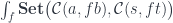
So the corollary to the Yoneda lemma in the functor category, after a few renamings, reads:

This is getting closer to the van Laarhoven formula because we have the end over functors, which is equivalent to

forall f. Functor f => ...

In fact, a judicious choice of and is all we need to finish the proof.

But sometimes it’s easier to define a functor indirectly, as an adjoint to another functor. Adjunctions actually allow us to switch categories. A functor defined by a mapping-out in one category can be adjoint to another functor defined by its mapping-in in another category.

A useful example is the currying adjunction in :

where corresponds to the function type a->y and, in , is isomorphic to the hom-set . This is just saying that a function of two arguments is equivalent to a function returning a function.

Here’s the clever trick: let’s replace and in the functorial Yoneda lemma with and , where and are some higher-order functors from to (as you will see, this notation anticipates the final substitution). We get:

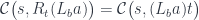
Now suppose that these functors are left adjoint to some other functors: and that go in the opposite direction from to . We can then replace all mappings-out in with the corresponding mappings-in in :

We are almost there! The last step is to realize that, in order to get the van Laarhoven formula, we need:

So these are just functors that apply to some fixed objects: and , respectively. The left-hand side becomes:

which is exactly the van Laarhoven representation.

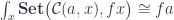
Now let’s look at the right-hand side:

We know what is, but what’s its left adjoint ? It must satisfy the adjunction:

or, using the end notation:

This identity has a simple solution when is , so we’ll just temporarily switch to . We have:

which is known as the IStore comonad in Haskell. We can check the identity by first applying the currying adjunction to eliminate the product:

and then using the Yoneda lemma to “integrate” over , which replaces with ,

So the right hand side of the original identity (after replacing with ) becomes:

which can be translated to Haskell as:

(s -> b -> t, s -> a)

or a pair of set and get.

I was very proud of myself for finding the right chain of substitutions, so I was pretty surprised when I learned from Mauro Jaskelioff and Russell O’Connor that they had a paper ready for publication with exactly the same proof. (They added a reference to my blog in their publication, which was probably a first.)

The Existentials

But there’s more: there are other optics for which this trick doesn’t work. The simplest one was the prism defined by a pair of functions:

match :: s -> Either t a
build :: b -> t

In this form it’s hard to see a commonality between a lens and a prism. There is, however, a way to unify them using existential types.

Here’s the idea: A lens can be applied to types that, at least conceptually, can be decomposed into two parts: the focus and the residue. It lets us extract the focus using get, and replace it with a new value using set, leaving the residue unchanged.

The important property of the residue is that it’s opaque: we don’t know how to retrieve it, and we don’t know how to modify it. All we know about it is that it exists and that it can be combined with the focus. This property can be expressed using existential types.

Symbolically, we would want to write something like this:

type Lens s t a b = exists c . (s -> (c, a), (c, b) -> t)

where c is the residue. We have here a pair of functions: The first decomposes the source s into the product of the residue c and the focus a . The second recombines the residue with the new focus b resulting in the target t.

Existential types can be encoded in Haskell using GADTs:

data Lens s t a b where
  Lens :: (s -> (c, a), (c, b) -> t) -> Lens s t a b

They can also be encoded in category theory using coends. So the lens can be written as:

The integral sign with the argument at the top is called a coend. You can read it as “there exists a ”.

There is a version of the Yoneda lemma for coends as well:

The intuition here is that, given a functorful of ‘s and a function c->a, we can fmap the latter over the former to obtain f a. We can do it even if we have no idea what the type c is.

We can use the currying adjunction and the Yoneda lemma to transform the new definition of the lens to the old one:

The exponential translates to the function type b->t, so this this is really the set/get pair that defines the lens.

The beauty of this representation is that it can be immediately applied to the prism, just by replacing the product with the sum (coproduct). This is the existential representation of a prism:

To recover the standard encoding, we use the mapping-out property of the sum:

This is simply saying that a function from the sum type is equivalent to a pair of functions—what we call case analysis in programming.

We get:

This has the form suitable for the use of the Yoneda lemma, namely:

with the functor

The result of the Yoneda is replacing with , so the result is:

which is exactly the match/build pair (in Haskell, the sum is translated to Either).

It turns out that every optic has an existential form.

Next: Profunctors.