What is algebra? Naively speaking algebra gives us the ability to perform calculations with numbers and symbols. Abstract algebra treats symbols as elements of a vector space: they can be multiplied by scalars and added to each other. But what makes algebras stand appart from linear spaces is the presence of vector multiplication: a bilinear product of vectors whose result is another vector (as opposed to inner product, which produces a scalar). Complex numbers, for instance, can be described as 2-d vectors, whose components are the real and the imaginary parts.

But nothing prepares you for this definition of F-algebra from the Haskell package Control.Functor.Algebra:

type Algebra f a = f a -> a

In this post I will try to bridge the gap between traditional algebras and more powerful F-algebras. F-algebras reduce the notion of an algebra to the bare minimum. It turns out that the three basic ingredients of an algebra are: a functor, a type, and a function. It always amazes me how much you can do with so little. In particular I will explain a very general way of evaluating arbitrary expressions using catamorphisms, which reduces to foldr when applied to lists (which can also be looked at as simple F-algebras).

The Essence of Algebra

There are two really essential aspects of an algebra:

  1. The ability to form expressions and
  2. The ability to evaluate these expressions

The Essence of Expression

The standard way of generating expressions is to use grammars. Here’s an example of a grammar in Haskell:

data Expr = Const Int
          | Add Expr Expr
          | Mul Expr Expr

Like most non-trivial grammars, this one is defined recursively. You may think of Expr as a self-similar fractal. An Expr, as a type, contains not only Const Int, but also Add and Mult, which inside contain Exprs, and so on. It’s trees all the way down.

1. The fractal nature of an expression type

But recursion can be abstracted away to uncover the real primitives behind expressions. The trick is to define a non-recursive function and then find its fixed point.

Since here we are dealing with types, we have to define a type function, otherwise known as type constructor. Here’s the non-recursive precursor of our grammar (later you’ll see that the F in ExprF stands for functor):

data ExprF a = Const Int
             | Add a a
             | Mul a a

The fractally recursive structure of Expr can be generated by repeatedly applying ExprF to itself, as in ExprF (ExprF (ExprF a))), etc. The more times we apply it, the deeper trees we can generate. After infinitely many iterations we should get to a fixed point where further iterations make no difference. It means that applying one more ExprF would’t change anything — a fixed point doesn’t move under ExprF. It’s like adding one to infinity: you get back infinity.

In Haskell, we can express the fixed point of a type constructor f as a type:

newtype Fix f = In (f (Fix f))

If you look at this formula closely, it is exactly what I said: Fix f is the type you get by applying f to itself. It’s a fixed point of f. (In the literature you’ll sometimes see Fix called Mu.)

We only need one generic recursive type, Fix, to be able to crank out other recursive types from (non-recursive) type constructors.

One thing to observe about the data constructor of Fix: In can be treated as a function that takes an element of type f (Fix f) and produces a Fix f:

In :: f (Fix f) -> Fix f

We’ll use this function later.

With that, we can redefine Expr as a fixed point of ExprF:

type Expr = Fix ExprF

You might ask yourself: Are there any values of the type Fix ExprF at all? Is this type inhabited? It’s a good question and the answer is yes, because there is one constructor of ExprF that doesn’t depend on a. This constructor is Const Int. We can bootstrap ourselves because we can always create a leaf Expr, for instance:

val :: Fix ExprF
val = In (Const 12)

Once we have that ability, we can create more and more complex values using the other two constructors of ExprF, as in:

testExpr = In $ (In $ (In $ Const 2) `Add` 
                (In $ Const 3)) `Mul` (In $ Const 4)

The Essence of Evaluation

Evaluation is a recipe for extracting a single value from an expression. In order to evaluate expressions which are defined recursively, the evaluation has to proceed recursively as well.

Again, recursion can be abstracted away — all we really need is an evaluation strategy for each top level construct (generated, for instance, by ExprF) and a way to evaluate its children. Let’s call this non-recursive top-level evaluator alg and the recursive one (for evaluating children) eval. Both alg and eval return values of the same type, a.

First, we need to be able to map eval over the children of an expression. Did somebody mentioned mapping? That means we need a functor!

Indeed, it’s easy to convince ourselves that our ExprF is a functor:

instance Functor ExprF where
    fmap f (Const i) = Const i
    fmap f (left `Add` right) = (f left) `Add` (f right)
    fmap f (left `Mul` right) = (f left) `Mul` (f right)

An F-algebra is built on top of a functor — any functor. (Strictly speaking, an endofunctor: it maps a given category into itself — in our examples the category refers to Hask — the category of all Haskell types).

Now suppose we know how to evaluate all the children of Add and Mul in an Expr, giving us values of some type a. All that’s left is to evaluate (Add a a) and (Mul a a) in ExprF a. (We also need to evaluate Const Int, but that doesn’t involve recursion.)

Here’s an example of such an evaluator that produces Int values:

alg :: ExprF Int -> Int

alg (Const i)   = i
alg (x `Add` y) = x + y
alg (x `Mul` y) = x * y

(Notice that we are free to add and multiply x and y, since they are just Ints.)

What I have done here is to pick one particular type, Int, as my evaluation target. This type is called the carrier type of the algebra. I then defined a function alg from the image of Int under the functor ExprF back to Int.

Just to show that the carrier type is arbitrary, let me define another evaluator that returns a string:

alg' :: ExprF String -> String

alg' (Const i)   = [chr (ord 'a' + i)]
alg' (x `Add` y) = x ++ y
alg' (x `Mul` y) = concat [[a, b] | a <- x, b <- y]

F-Algebras

We are now ready to define F-algebras in the most general terms. First I’ll use the language of category theory and then quickly translate it to Haskell.

An F-algebra consists of:

  1. an endofunctor F in a category C,
  2. an object A in that category, and
  3. a morphism from F(A) to A.

An F-algebra in Haskell is defined by a functor f, a carrier type a, and a function from (f a) to a. (The underlying category is Hask.)

Right about now the definition with which I started this post should start making sense:

type Algebra f a = f a -> a

For a given functor f and a carrier type a the alebra is defined by specifying just one function. Often this function itself is called the algebra, hence my use of the name alg in previous examples.

Back to our conrete example, the functor is ExprF, the carrier type is Int and the function is alg:

-- My simple algebra
type SimpleA = Algebra ExprF Int

alg :: SimpleA
alg (Const i)   = i
alg (x `Add` y) = x + y
alg (x `Mul` y) = x * y

The only thing that’s still missing is the definition of the function eval, which takes care of evaluating children of an expression. It turns out this function can be defined in a very general form. To do that we’ll need to familiarize ourselves with the notion of the initial algebra.

Initial Algebras

There are many algebras based on a given functor (I’ve shown you two so far). But there is one algebra to bind them all — the initial algebra. In fact you’ve already seen elements of it. Remember the Fix type function?

newtype Fix f = In (f (Fix f))

Given any functor f it defines a new unique type Fix f. We will now lift ourselves by the bootstraps. We’ll use this type as a carrier in the definition of another algebra. This will turn out to be our initial algebra.

First, let’s go back to our example and, instead of using Int or String, use (Fix ExprF) as the carrier type:

type ExprInitAlg = Algebra ExprF (Fix ExprF)

We have the functor and the carrier type. To complete the triple we need to define a function with the following signature:

ex_init_alg :: ExprF (Fix ExprF) -> Fix ExprF

Guess what, we already have a function of this type. It’s the constructor of Fix:

ex_init_alg = In

(Replace f with ExprF in the definition of Fix to see that the type signatures match.)

But wait! What does this “evaluator” evaluate? Given (ExprF Expr) it produces an Expr. For instance, when given,

Add (In $ Const 2) (In $ Const 3)

it will produce an Expr:

In $ Add (In $ Const 2) (In $ Const 3)

This evaluator doesn’t reduce anything like the evaluators we’ve been using so far. It is not lossy. It preserves all the information passed to it as input. [Note: In fact, Lambek’s lemma states that the initial algebra is an isomorphism.] In comparison, all other evaluators potentially lose some information. They return some kind of summary of the information encoded in the data structure. In this sense, the algebra we have just defined is at least as powerful as all other algebras based on the same functor. That’s why it’s called the initial algebra.

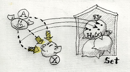
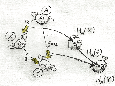
The word initial has a special meaning in category theory. The initial algebra has the property that there exists a (unique) homomophism from it to any other algebra based on the same functor.

A homomoprhism is a mapping that preserves certain structure. In the case of algebras, a homomorphism has to preserve the algebraic structure. An algebra consists of a functor, a carrier type, and an evaluator. Since we are keeping the functor fixed, we only need to map carrier types and evaluators.

In fact, a homomorphism of algebras is fully specified by a function that maps one carrier to another and obeys certain properties. Since the carrier of the intial algebra is Fix f, we need a function:

g :: Fix f -> a

where a is the carrier for the other algebra. That algebra has an evaluator alg with the signature:

alg :: f a -> a

2. Homomorphism from the initial algebra to an arbitrary algebra

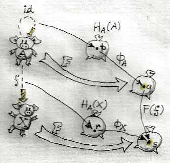
The special property g has to obey is that it shouldn’t matter whether we first use the initial algebra’s evaluator and then aply g, or first apply g (through fmap) and then the second algebra’s evaluator, alg. Let’s check the types involved to convince ourselves that this requirement makes sense.

The first evaluator uses In to go from f (Fix f) to Fix f. Then g takes Fix f to a.

The alternate route uses fmap g to map f (Fix f) to f a, followed by alg from f a to a. Notice that this is the first time that we used the functorial property of f. It allowed us to lift the function g to fmap g.

The crucial observation is that In is a losless transformation and it can be easily inverted. The inverse of In is unFix:

unFix :: Fix f -> f (Fix f)
unFix (In x) = x

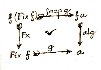
With one reversal of the arrow In to unFix, it’s easy to see that going the route of g is the same as taking the detour through unFix, followed by fmap g, and then alg:

3. Defining a catamorphism

g = alg . (fmap g) . unFix

We can use this equation as a recursive definition of g. We know that this definition converges because the application of g through fmap deals with subtrees of the original tree, and they are strictly smaller than the original tree.

We can abstract the evaluation further by factoring out the dependence on alg (redefining g = cata alg):

cata :: Functor f => (f a -> a) -> Fix f -> a
cata alg = alg . fmap (cata alg) . unFix

The result is a very generic function called a catamorphism. We have constructed the catamorphism from an algebra in order to prove that the fixed point of this algebra’s functor is the initial algebra. But wait, haven’t we just created the recursive evaluator we’ve been looking for?

Catamorphisms

Look again at the type signature of the catamorphism with some additional (redundant) parentheses:

cata :: Functor f => (f a -> a) -> (Fix f -> a)

It takes an arbitrary algebra, which is a non-recursive function f a -> a, and returns an evaluator function, (Fix f -> a). This function takes an expression of the type Fix f and evaluates it down to type a. A catamorphism lets us evaluate arbitrarily nested expressions!

Let’s try it with our simple functor ExprF, which we used to generate nested expressions of the type Fix ExprF.

We have already defined an alg for it:

type SimpleA = Algebra ExprF Int

alg :: SimpleA
alg (Const i)   = i
alg (x `Add` y) = x + y
alg (x `Mul` y) = x * y

So our full-blown evaluator is just:

eval :: Fix ExprF -> Int
-- eval = cata alg = alg . fmap (cata alg) . unFix
eval = alg . fmap eval . unFix

Let’s analyze it: First, unFix allows us to peek at the top level of the input expression: It’s either a leaf Const i or an Add or Mul whose children are, again, full-blown expression, albeit one degree shallower. We evaluate the children by recursively applying eval to them. We end up with a single level tree whose leaves are now evaluated down to Ints. That allows us to apply alg and get the result.

You can test this on a sample expression:

testExpr = In $ (In $ (In $ Const 2) `Add` 
                (In $ Const 3)) `Mul` (In $ Const 4)

You can run (and modify) this code online in the School of Haskell version of this blog.

{-# LANGUAGE DeriveFunctor #-}
data ExprF r = Const Int
             | Add r r
             | Mul r r
    deriving Functor

newtype Fix f = In (f (Fix f))
unFix :: Fix f -> f (Fix f)
unFix (In x) = x

cata :: Functor f => (f a -> a) -> Fix f -> a
cata alg = alg . fmap (cata alg) . unFix

alg :: ExprF Int -> Int
alg (Const i)   = i
alg (x `Add` y) = x + y
alg (x `Mul` y) = x * y

eval :: Fix ExprF -> Int
eval = cata alg

testExpr = In $ 
             (In $ (In $ Const 2) `Add` (In $ Const 3)) `Mul` 
             (In $ Const 4)

main = print $ eval $ testExpr

foldr

Traversing and evaluating a recursive data structure? Isn’t that what foldr does for lists?

Indeed, it’s easy to create algebras for lists. We start with a functor:

data ListF a b = Nil | Cons a b

instance Functor (ListF a) where
    fmap f Nil = Nil
    fmap f (Cons e x) = Cons e (f x)

The first type argument to ListF is the type of the element, the second is the one we will recurse into.

Here’s a simple algebra with the carrier type Int:

algSum :: ListF Int Int -> Int
algSum Nil = 0
algSum (Cons e acc) = e + acc

Using the constructor In we can recursively generate arbitrary lists:

lst :: Fix (ListF Int)
lst = In $ Cons 2 (In $ Cons 3 (In $ Cons 4 (In Nil)))

Finally, we can evaluate our list using our generic catamorphism:

cata algSum lst

Of course, we can do exactly the same thing with a more traditional list and foldr:

foldr (\e acc -> e + acc) 0 [2..4]

You should see the obvious paralles between the definition of the algSum algebra and the two arguments to foldr. The difference is that the algebraic approach can be generalized beyond lists to any recursive data structure.

Here’s the complete list example:

newtype Fix f = In (f (Fix f))

unFix :: Fix f -> f (Fix f)
unFix (In x) = x

cata :: Functor f => (f a -> a) -> Fix f -> a
cata alg = alg . fmap (cata alg) . unFix

data ListF a b = Nil | Cons a b

instance Functor (ListF a) where
    fmap f Nil = Nil
    fmap f (Cons e x) = Cons e (f x)

algSum :: ListF Int Int -> Int
algSum Nil = 0
algSum (Cons e acc) = e + acc

lst :: Fix (ListF Int)
lst = In $ Cons 2 (In $ Cons 3 (In $ Cons 4 (In Nil)))

main = do
    print $ (cata algSum) lst
    print $ foldr (\e acc -> e + acc) 0 [2, 3, 4]

Conclusion

Here are the main points of this post:

  1. Just like recursive functions are defined as fixed points of regular functions, recursive (nested) data structures can be defined as fixed points of regular type constructors.
  2. Functors are interesting type constructors because they give rise to nested data structures that support recursive evaluation (generalized folding).
  3. An F-algebra is defined by a functor f, a carrier type a, and a function from f a to a.
  4. There is one initial algebra that maps into all algebras defined over a given functor. This algebra’s carrier type is the fixed point of the functor in question.
  5. The unique mapping between the initial algebra and any other algebra over the same functor is generated by a catamorphism.
  6. Catamophism takes a simple algebra and creates a recursive evaluator for a nested data structure (the fixed point of the functor in question). This is a generalization of list folding to arbitrary recursive data structures.

Acknowledgment

I’m greatful to Gabriel Gonzales for reviewing this post. Gabriel made an interesting observation:

“Actually, even in Haskell recursion is not completely first class because the compiler does a terrible job of optimizing recursive code. This is why F-algebras and F-coalgebras are pervasive in high-performance Haskell libraries like vector, because they transform recursive code to non-recursive code, and the compiler does an amazing job of optimizing non-recursive code.”

Bibliography

Most examples in my post were taken from the first two publications below:

  1. Fixing GADTs by Tim Philip Williams.
  2. Advanced Functional Programming, Tim Sheard’s course notes.
  3. Functional Programming with Bananas, Lenses, Envelopes, and Barbed Wire by Erik Meijer, Maarten Fokkinga, and Ross Paterson.
  4. Recursive types for free! by Philip Wadler
  5. Catamorphisms in Haskell Wiki

You don’t need to know anything about category theory to use Haskell as a programming language. But if you want to understand the theory behind Haskell or contribute to its development, some familiarity with category theory is a prerequisite.

Category theory is very easy at the beginning. I was able to explain what a category is to my 10-year old son. But the learning curve gets steeper as you go. Functors are easy. Natural transformations may take some getting used to, but after chasing a few diagrams, you’ll get the hang of it. The Yoneda lemma is usually the first serious challenge, because to understand it, you have to be able to juggle several things in your mind at once. But once you’ve got it, it’s very satisfying. Things just fall into place and you gain a lot of intuition about categories, functors, and natural transformations.

A Teaser Problem

You are given a polymorphic function imager that, for any function from Bool to any type r, returns a list of r. Try running this code in the School of Haskell, with colorMap, heatMap, and soundMap. You may also define your own function of Bool and pass it to imager.

{-# LANGUAGE ExplicitForAll #-}
imager :: forall r . ((Bool -> r) -> [r])
imager = ???

data Color = Red | Green | Blue        deriving Show
data Note  = C | D | E | F | G | A | B deriving Show

colorMap x = if x then Blue else Red
heatMap  x = if x then 32   else 212
soundMap x = if x then C    else G

main = print $ imager colorMap

Can you guess the implementation of imager? How many possible imagers with the same signature are there? By the end of this article you should be able to validate your answers using the Yoneda’s lemma.

Categories

A category is a bunch of objects with arrows between them (incidentally, a “bunch” doesn’t mean a set but a more generall collection). We don’t know anything about the objects — all we know is the arrows, a.k.a morphisms.

Our usual intuition is that arrows are sort of like functions. Functions are mappings between sets. Indeed, morphisms have some function-like properties, for instance composability, which is associative:

Fig 1. Associativity of morphisms demonstrated on Haskell functions. (In my pictures, piggies will represent objects; sacks of potatoes, sets; and fireworks, morphisms.)

h :: a -> b
g :: b -> c
f :: c -> d

f . (g . h) == (f . g) . h

There is also an identity morphism for every object in a category, just like the id function:

Fig 2. The identity morphism.

id :: a -> a

id . f == f . id == f

In all Haskell examples I’ll be using the category Hask of Haskell types, with morphisms being plain old functions. An object in Hask is a type, like Int, [Bool], or [a]->Int. Types are nothing more than just sets of values. Bool is a two element set {True, False}, Integer is the set of all integers, and so on.

In general, a category of all sets and functions is called Set .

So how good is this sets-and-functions intuition for an arbitrary category? Are all categories really like collections of sets, and morphisms are like functions from set to set? What does the word like even mean in this context?

Functors

In category theory, when we say one category is “like” another category, we usually mean that there is a mapping between the two. For this mapping to be meaningful, it should preserve the structure of the category. So not only every object from one category has to be mapped into an object from another category, but also all morphisms must be mapped correctly — meaning they should preserve composition. Such a mapping has a name: it’s called a functor.

Functors in Hask are described by the type class Functor

class Functor f where
fmap :: (a -> b) -> (f a -> f b)

A Haskell Functor maps types into types and functions into functions — a type constructor does the former and fmap does the latter.

A type contructor is a mapping from one type to another. For instance, a list type constructor takes any type a and creates a list type, [a].

So instead of asking if every category is “like” the Set category, we can ask a more precise question: For what types of categories (if not all of them) there exist functors that map them into Set . Such categories are called representable, meaning they have a representation in Set .

As a physicist I had to deal a lot with groups, such as groups of spacetime rotations in various dimensions or unitary groups in complex spaces. It was very handy to represent these abstract groups as matrices acting on vectors. For instance, different representations of the same Lorenz group (more precisely, SL(2, C)) would correspond to physical particles with different spins. So vector spaces and matrices are to abstract groups as sets and functions are to abstract categories.

Yoneda Embedding

One of the things Yoneda showed is that there is at least one canonical functor from any so called locally small category into the category of sets and functions. The construction of this functor is surpisingly easy, so let me sketch it.

This functor should map every object in category C into a set. Set of what? It doesn’t really matter, a set is a set. So how about using a set of morphisms?

Fig 3. The Yoneda embedding. Object X is mapped by the functor into the set HA(X). The elements of the set correspond to morphisms from A to X.

How can we map any object into a set of morphisms? Easy. First, let’s arbitrarily fix one object in the category C, call it A. It doesn’t matter which object we pick, we’ll just have to hold on to it. Now, for every object X in C there is a set of morphisms (arrows) going from our fixed A to this X. We designate this set to be the image of X under the functor we are constructing. Let’s call this functor HA. There is one element in the set HA(X) for every morphism from A to X.

A functor must define a mapping of objects to objects (to sets, in our case) and morphisms to morphisms (to functions in our case). We have established the first part of the mapping. To define the second part, let’s pick an arbitrary morphism f from X to Y. We have to map it to some function from the set HA(X) to the set HA(Y).

Fig 4. The Yoneda functor also maps morphisms. Here, morphism f is mapped into the function HA(f) between sets HA(X) and HA(Y).

Let’s define this function, we’ll call it HA(f), through its action on any element of the set HA(X), call it x. By our construction, x corresponds to some particular morphism, u, from A to X. We now have at our disposal two morphisms, u :: A -> X and f :: X -> Y (that’s the morphism we are mapping). We can compose them. The result f . u is a morphism from A to Y, so it’s a member of the set HA(Y). We have just defined a function that takes an x from HA(X) and maps it into y from HA(Y), and this will be our HA(f).

Of course, you have to prove that this construction of HA is indeed a functor preserving composition of morphisms, but that’s reasonably easy, once the technique we have just used becomes familiar to you. Here’s the gist of this technique: Use components! When you are defining a functor from category C to category D, pick a component — an object X in C — and define its image, F(X). Then pick a morphism f in C, say from X to Y, and define its image, F(f), as a particular morphism from F(X) to F(Y).

Similarly, when defining a function from set S to T, use its components. Pick an element x of S and define its image in T. That’s exactly what we did in our construction.

Incidentally, what was that requirement that the category C be locally small? A category is locally small if the collection of morphisms between any two objects forms a set. This may come as a surprise but there are things in mathematics that are too big to be sets. A classic example is a collection of all sets, which cannot be a set itself, because it would lead to a paradox. A collection of all sets, however, is the basis of the Set category (which, incidentally, turns out to be locally small).

Summary So Far

Let me summarize what we’ve learned so far. A category is just a bunch of abstract objects and arrows between them. It tells us nothing about the internal structure of objects. However, for every (locally small) category there is a structure-preserving mapping (a functor) that maps it into a category of sets. Objects in the Set category do have internal structure: they have elements; and morphisms are functions acting on those elements. A representation maps the categorie’s surface structure of morphisms into the internal structure of sets.

It is like figuring out the properties of orbitals in atoms by looking at the chemical compounds they form, and at the way valencies work. Or discovering that baryons are composed of quarks by looking at their decay products. Incidentally, no one has ever “seen” a free quark, they always live inside other particles. It’s as if physicists were studying the “category” of baryons by mapping them into sets of quarks.

A Bar Example

This is all nice but we need an example. Let’s start with “A mathematician walks into a bar and orders a category.” The barman says, “We have this new tasty category but we can’t figure out what’s in it. All we know is that it has just one object A” — (“Oh, it’s a monoid,” the mathematician murmurs knowingly) — “…plus a whole bunch of morphisms. Of course all these morphisms go from A to A, because there’s nowhere else to go.”

What the barman doesn’t know is that the new category is just a re-packaging of the good old set of ASCII strings. The morphisms correspond to appending strings. So there is a morphism called foo that apends the string "foo"

foo :: String -> String
foo = (++"foo")

main = putStrLn $ foo "Hello "

and so on.

“I can tell you what’s inside A,” says the mathematician, “but only up to an isomorphism. I’m a mathematician not a magician.”

She quickly constructs a set that contains one element for each morphism — morphisms must, by law, be listed by the manufacturer on the label. So, when she sees foo, she puts an element with the label “foo”, and so on. Incidentally, there is one morphism with no name, which the mathematician maps to an empty label. (In reality this is an identity morphism that appends an empty string.)

“That’s what’s inside the object A,” she says.

“Moreover, this set comes equipped with functions that rearrange its elements. In fact there is a function for every morphism listed in the category,” she says. “Name any morphism and I’ll construct you a function.”

The barman gives her morphism p, which in reality is:

p = (++"p")

“Okay,” she says, “here’s how I construct the corresponding function. Pick any element in my set.”

The barman picks “foo”.

“Okay, ‘foo’ corresponds to the morphism foo,” she says, “so tell me what you call the morphism that’s the composition of foo and p?” (By law, the manufacturer is obliged to specify all admissible compositions of morphisms on the label.)

“It’s called foop,” says the barman.

Quick check:

p . foo == (++"p") . (++"foo") == (++"foop")
foop = (++"foop")

“Okay,” she says, “the function corresponding to p maps “foo” into “foop”. Hm, how curious! I bet this function will map the no-label elment into “p”, is that right?”

“Indeed, it does,” says the barman.

Quick check:

p . id == p

“I bet you this is just a string monoid,” says the mathematician.

“I think I’ll have my usual Top on the rocks instead.”

Natural Transformations

We’ve seen how to construct a representation of any (locally small) category in Set by selecting an arbitrary object A in the category and studying morphisms originating at A. What if we choose a different object B instead? How different is the representation HA from HB? For that matter, what if we pick any functor F from C to Set ? How is it related to HA? That’s what the Yoneda lemma is all about.

Let me start with a short recap.

A functor is a mapping between categories that preserves their structure. The structure of a category is defined by the way its morphisms compose. A functor F maps objects into objects and morphism into morphisms in such a way that if f . g = h then F(f) . F(g) = F(h).

A natural transformation is a mapping between functors that preserves the structure of the underlying categories.

Fig 5. A component of a transformation Φ at X. Φ maps functor F into functor G, ΦX is a morphism that maps object F(X) into object G(X).

First we have to understand how to define mappings between functors. Suppose we have functors F and G, both going from category C to category D. For a given object X in C, F will map it into F(X) in D, and G will map it into G(X) in D. A mapping Φ between functors must map object F(X) to object G(X), both in category D. We know that a mapping of objects is called a morphism. So for every object X we have to provide a morphism ΦX from F(X) to G(X). This morphism is called a component of Φ at X. Or, looking at it from a different angle, Φ is a family of morphisms parameterized by X.

An Example of Natural Transformation

Just to give you some Haskell intuition, consider functors on Hask . These are mapping of types (type constructors) such as a -> [a] or a -> Maybe a, with the corresponging mappings of morphisms (functions) defined by fmap. Recall:

class Functor f where
fmap :: (a -> b) -> (f a -> f b)

The mapping between Haskell functors is a family of functions parameterized by types. For instance, a mapping between the [] functor and the Maybe functor will map a list of a, [a] into Maybe a. Here’s an example of such a family of functions called safeHead:

safeHead :: [a] -> Maybe a
safeHead []     = Nothing
safeHead (x:xs) = Just x

A family of functions parameterized by type is nothing special: it’s called a polymorphic function. It can also be described as a function on both types and values, with a more verbose signature:

{-# LANGUAGE ExplicitForAll #-}

safeHead :: forall a . [a] -> Maybe a
safeHead []     = Nothing
safeHead (x:xs) = Just x

main = print $ safeHead ["One", "Two"]

Let’s go back to natural transformations. I have described what it means to define a transformation of functors in terms of objects, but functors also map morphism. It turns out, however, that the tranformation of morphisms is completely determined by the two functors. A morphism f from X to Y is transformed under F into F(f) and under G into G(f). G(f) must therefore be the image of F(f) under Φ. No choice here! Except that now we have two ways of going from F(X) to G(Y).

Fig 6. The naturality square. Φ is a natural transformation if this diagram commutes, that is, both paths are equivalent.

We can first use the morphism F(f) to take us to F(Y) and then use ΦY to get to G(Y). Or we can first take ΦX to take us to G(X), and then G(f) to get to G(Y). We call Φ a natural transformation if these two paths result in the same morphism (the diagram commutes).

The best insight I can offer is that a natural transformation works on structure, while a general morphism works on contents. The naturality condition ensures that it doesn’t matter if you first rearrange the structure and then the content, or the other way around. Or, in other words, that a natural transformation doesn’t touch the content. This will become clearer in examples.

Going back to Haskell: Is safeHead a natural transformation between two functors [] and Maybe? Let’s start with a function f from some type a to b. There are two ways of mapping this function: one using the fmap defined by [], which is the list function map; and the other using the Maybe‘s fmap, which is defined in the Maybe‘s functor instance definition:

instance Functor Maybe where
   fmap f (Just x) = Just (f x)
   fmap _ Nothing  = Nothing

The two path from [a] to Maybe b are:

  1. Apply fmap f to [a] to get [b] and then safeHead it, or
  2. Apply safeHead to [a] and then use the Maybe version of fmap.

There are only two cases to consider: an empty list and a non-empty list. For an emtpy list we get Nothing both ways, otherwise we get Just f acting on the first element of the list.

We have thus shown that safeHead is a natural transformation. There are more interestig examples of natural transformations in Haskell; monadic return and join come to mind.

The intuition behind natural transformations is that they deal with structure, not contents. safeHead couldn’t care less about what’s stored in a list, but it understands the structure of the list: things like the list being empty, or having a first element. The type of this element doesn’t matter. In Haskell, natural transformations are polymorphic functions that can, like safeHead be typed using forall:

safeHead :: forall a . [a] -> Maybe a

Yoneda Lemma

Going back to the Yoneda lemma, it states that for any functor from C to Set there is a natural transformation from our canonical representation HA to this functor. Moreover, there are exactly as many such natural transformations as there are elements in F(A).

That, by the way, answers our other question about the dependence on the choice of A in the Yoneda embedding. The Yoneda lemma tells us that there are natural transformations both ways between HA and HB.

Amazingly, the proof of the Yoneda lemma, at least in one direction, is quite simple. The trick is to first define the natural transformation Φ on one special element of HA(A): the element that corresponds to the identity morphism on A (remember, there is always one of these for every object). Let’s call this element p. Its image under ΦA will be in F(A), which is a set. You can pick any element of this set and it will define a different but equally good Φ. Let’s call this element q. So we have fixed ΦA(p) = q.

Now we have to define the action of Φ on an arbitrary element in the image of HA. Remember that the functor HA transforms objects in C into sets. So let’s take an arbitrary object X and its image HA(X). The elements in HA(X) correspond to morphisms from A to X. So let’s pick one such morphism and call it f. Its image is an element r in HA(X). The question is, what does r map into under Φ? Remember, it’s image must be an element of F(X).

Fig 7. The mappings in the Yoneda lemma. F is an arbitrary functor. Any choice of p determines the morphism ΦX for any X.

To figure that out, let’s consider the F route. F being a functor transforms our morphism f into F(f) — which is a morphism from F(A) to F(X). But, as you may remember, we have selected a special element in F(A) — our q. Now apply F(f) to q and you get an element in F(X), call it s. (Remember, F(f) is just a regular function between two sets, F(A) and F(X).)

There’s nothing more natural than picking ΦX(r) to be this s! We have thus defined a natural transformation Φ for any X and r.

The straightforward proof that this definition of Φ is indeed natural is left as an exercise to the user.

A Haskell Example

I’ve been very meticulous about distinguishing between morphisms from A to X in C and the corresponding set elements in HA(X). But in practice it’s more convenient to skip the middle man and define natural transformations in the Yoneda lemma as going directly from these morphisms to F(X). Keeping this in mind, the Haskell version of the Yoneda lemma is ofter written as follows:

forall r . ((a -> r) -> f r) ~ f a

where the (lowercase) f is the functor (think of it as a type constructor and its corresponding fmap), (a -> r) is a function corresponding to the morphism from A to X in our orginal formulation. The Yoneda’s natural transformation maps this morphism into the image of r under f — the F(X) in the original formulation. The forall r means that the function ((a -> r) -> f r) works for any type r, as is necessary to make it a natural transformation.

The lemma states that the type of this function, forall r . ((a -> r) -> f r) is equivalent to the much simpler type f a. If you remember that types are just sets of values, you can interpret this result as stating that there is one-to-one correspondence between natural transformations and values of the type f r.

Remember the example from the beginning of this article? There was a function imager with the following signature:

imager :: forall r . ((Bool -> r) -> [r])

This looks very much like a natural transformation from the Yoneda lemma with the type a fixed to Bool and the functor, the list functor []. (I’ll call the functions Bool->r iffies.)

The question was, how many different implementations of this signature are there?

The Yoneda lemma tells us exactly how to construct such natural transformations. It instructs us to start with an identity iffie: idBool :: Bool -> Bool, and pick any element of [Bool] to be its image under our natural transformation. We can, for instance, pick [True, False, True, True]. Once we’ve done that, the action of this natural transformation on any iffie h is fixed. We just map the morphism h using the functor (in Haskell we fmap the iffie), and apply it to our pick, [True, False, True, True].

Therefore, all natural transformations with the signature:

forall r . ((Bool -> r) -> [r])

are in one-to-one correspondence with different lists of Bool.

Conversely, if you want to find out what list of Bool is hidden in a given implementation of imager, just pass it an identity iffie. Try it:

{-# LANGUAGE ExplicitForAll #-}

imager :: forall r . ((Bool -> r) -> [r])
imager iffie = fmap iffie [True, False, True, True]

data Color = Red | Green | Blue        deriving Show
data Note  = C | D | E | F | G | A | B deriving Show

colorMap x = if x then Blue else Red
heatMap  x = if x then 32   else 212
soundMap x = if x then C    else G
idBool :: Bool -> Bool
idBool x = x

main = print $ imager idBool

Remember, this application of the Yoneda lemma is only valid if imager is a natural transformation — its naturality square must commute. The two functors in the imager naturality diagram are the Yoneda embedding and the list functor. Naturality of imager translates into the requirement that any function f :: a -> b modifying an iffie could be pulled out of the imager:

imager (f . iffie) == map f (imager iffie)

Here’s an example of such a function translating colors to strings commuting with the application of imager:

{-# LANGUAGE ExplicitForAll #-}

imager :: forall r . ((Bool -> r) -> [r])
imager iffie = fmap iffie [True, False, True, True]

data Color = Red | Green | Blue  deriving Show

colorMap x = if x then Blue else Red

f :: Color -> String
f = show 

main = do
    print $ imager (f . colorMap)
    print $ map f (imager colorMap)

The Structure of Natural Transformations

That brings another important intuition about the Yoneda lemma in Haskell. You start with a type signature that describes a natural transformation: a particular kind of polymorphic function that takes a probing function as an argument and returns a type that’s the result of a functor acting on the result type of the probing function. Yoneda tells us that the structure of this natural transformation is tightly constrained.

One of the strengths of Haskell is its very strict and powerful type system. Many Haskell programers start designing their programs by defining type signatures of major functions. The Yoneda lemma tells us that type signatures not only restrict how functions can be combined, but also how they can be implemented.

As an extreme, there is one particular signature that has only one implementation: a->a (or, more explicitly, forall a. a -> a). The only natural implementation of this signature is the identity function, id.

Just for fun, let me sketch the proof using the Yoneda lemma. If we pick the source type as the singleton unit type, (), then the Yoneda embedding consists of all functions taking unit as an argument. A function taking unit has only one return value so it’s really equivalent to this value. The functor we pick is the identity functor. So the question is, how many natural tranformation of the the following type are there?

forall a. ((() -> a) -> a)

Well, there are as many as there are elements in the image of () under the identity functor, which is exactly one! Since a function ()->a can be identified with a, it means we have only one natural transformation with the following signature:

forall a. (a -> a)

Moreover, by Yoneda construction, this function is defined by fmapping the function ()->a over the element () using the identity functor. So our natural transformation, when probed with a value of the type a will return the same value. But that’s just the definition of the identity function. (In reality things are slightly more complicated because every Haskell type must include undefined, but that’s a different story.)

Here’s an exercise for the reader: Show that the naturality square for this example is equivalent to id commuting with any function: f . id == id . f.

Conclusion

I hope I provided you with enough background information and intuition so that you’ll be able to easily read more advanced blog posts, like this one:
Reverse Engineering Machines with the Yoneda Lemma by Dan Piponi, or GADTs by Gabriel Gonzales.

Acknowledgments

I’d like to thank Gabriel Gonzales for providing useful comments and John Wiegley, Michael Sloan, and Eric Niebler for many interesting conversations.


I’ve been dealing with concurrency for many years in the context of C++ and D (see my presentation about Software Transactional Memory in D). I worked for a startup, Corensic, that made an ingenious tool called Jinx for detecting data races using a lightweight hypervisor. I recorded a series of screencasts teaching concurrency to C++ programmers. If you follow these screencasts you might realize that I was strongly favoring functional approach to concurrency, promoting immutability and pure functions. I even showed how non-functional looking code leads to data races that could be detected by (now defunct) Jinx. Essentially I was teaching C++ programmers how to imitate Haskell.

Except that C++ could only support a small subset of Haskell functionality and provide no guarantees against even the most common concurrency errors.

It’s unfortunate that most programmers haven’t seen what Haskell can do with concurrency. There is a natural barrier to learning a new language, especially one that has the reputation of being mind boggling. A lot of people are turned off simply by unfamiliar syntax. They can’t get over the fact that in Haskell a function call uses no parentheses or commas. What in C++ looks like

f(x, y)

in Haskell is written as:

f x y

Other people dread the word “monad,” which in Haskell is essentially a tool for embedding imperative code inside functional code.

Why is Haskell syntax the way it is? Couldn’t it have been more C- or Java- like? Well, look no farther than Scala. Because of Java-like syntax the most basic functional trick, currying a function, requires a Scala programmer to anticipate this possibility in the function definition (using special syntax: multiple pairs of parentheses). If you have no access to the source code for a function, you can’t curry it (at least not without even more syntactic gymnastics).

If you managed to wade through this post so far, you are probably not faint of heart and you will accept the challenge of reading an excellent article by Simon Peyton Jones, Beautiful Concurrency that does a great job of explaining to the uninitiated Haskell’s beautiful approach to concurrency. It’s not a new article, but it has been adapted to the new format of the School of Haskell by Yours Truly, which means you’ll be able to run code examples embedded in it. If you feel adventurous, you might even edit them and see how the results change.


Anybody who tries to popularize Haskell has to deal with the monad problem. You can’t write the simplest Haskell program without a monad (the IO monad in particular) and yet there is no easy way to explain what a monad is. Mind you, when teaching object oriented programming, nobody starts with a definition of “object.” There’s no need for that because everybody has some intuition about objects — we are surrounded by objects in real life. Which is very convenient because if you tried to define what an object is in C++ or Java, you’d have to use quite a bit of hard-core PL theory; plus you’d have to wave your hands a lot. This trick doesn’t work with monads because, except for category theorists, nobody comes to Haskell with any intuitions about monads. The name monad is scary in itself (this is probably why monads in F# are innocuously called “computation expressions”).

In my n’th attempt to tackle monads I tried a different, mystical, approach. In mysticism you often talk about things that you cannot define. Taoism takes this approach to the extreme — any attempt to define Tao must fail: “Tao that can be described is not the eternal Tao.” Hence the slightly tongue-in-cheek approach I took in this tutorial, Pure Functions, Laziness, I/O, and Monads. If you’re new to Haskell, it might help if you read the two previous tutorials in my Basics of Haskell. Notice that these tutorials are in the new format introduced by the School of Haskell, where you can run and edit program snippets directly in your browser.

I must confess that this tutorial got slightly cold welcome in the Haskell community. That’s why I’m curious what non-Haskellers think of it. Does my approach make monads less or more scary? Take into account that I decided to tackle monads right after explaining the very basics of Haskell syntax — in most courses or books monads are treated as an advanced topic.


At last I can start blabbing about it. The School of Haskell went beta. We’ve been working on it for the last half a year with a team of top-notch Haskell programmers.

Our main effort is to create an online Haskell IDE, but the technology we’ve been developing for it was just aching to be used for teaching Haskell. Imagine an online tutorial where snippets of code can be compiled and run on the spot. You can play with them: edit, compile, and run with your changes. You can pull instant documentation for any library function used in the snippet. Yup! And there’s more. Read the blog I linked to above and sign up for beta. It’s a great opportunity to fulfill you New Year’s resolution to finally learn Haskell or to create some Haskell content yourself. Enjoy!


2013 starts on a very positive note: Simon Peyton-Jones has just endorsed our company, FP Complete. And, as the saying goes, he put his money where his mouth is: He invested his own money in FP Complete. Here’s what he wrote about us in his blog:

Of course, FP Complete thereby faces the challenge of making a business out of a language ecosystem, something known to be difficult! Here I am encouraged by the fact that Aaron and Bartosz are not, like many of us, primarily techno-geeks whose primary motivation is the technology itself (just read the Haskell Weekly News if you have any doubt what I mean). They are excited by Haskell all right, but they want to build a business, and they have experience of doing just that. And I’m very encouraged by the fact that Michael Snoyman (a giant of the Haskell community) has joined them, along with several others.

Of course, if you’ve been following my blogs you know that I am a techno-geek too. You might have noticed a slow evolution in my interests from the messiness of C++ and its template metaprogramming, through a flirt with the D language, the pitfalls of concurrency and parallelism, to the clarity and robustness of Haskell. If I was able to entice some of you to make some of this journey with me, it makes me very happy.

But, as Simon PJ pointed out, loving a language and having fun with it is not the same as creating a successful business. Aaron (the CEO) and I have been spending a lot of time discussing business strategies. Everything we do is a deliberate step towards self-sustainability and profitability. All our work would be for naught if we couldn’t create a steady stream of revenue. It is a tremendous task, but we have experience and we are quick learners. We talk to companies to help them figure out how they can improve their bottom lines using Haskell. We identify the obstacles in the way of adoption of Haskell and help overcome them. If we can tap into even a small percentage of profits that the industry will make by adopting Haskell, our future is secured. And Simon P-J may stay assured that his investment will pay back manyfold.


I published a new blog post at the FP Complete site, with a peek at our efforts to create the Haskell IDE. I concentrated mostly on the interaction between the programmer and the IDE. I’ve been always championing the top-down approach to design and implementation — in the case of a GUI program, the top is the GUI. Of course we’ve been working on the infrastructure as well, but user experience is what makes or breaks software products.


A web programmer must be fluent in at least four languages: HTML, CSS, JavaScript, and a fourth language for writing server code. There’s nothing wrong with having specialized domain-specific languages — the problem is, they don’t fit together nicely. This is why a web developer has to learn the fifth language — the language of the application he or she uses to put together a web site. There are many such applications and each comes with a large set of rules and conventions. These applications are as flexible as their designers made them. They make common patterns easy to implement, but they don’t help with general programmability. For that you need a programming language, not an environment.

The idea behind the Yesod framework is to use an existing language, Haskell, to unify all aspects of web programming. There are many reasons why a functional language is a great fit for web programming — for instance, the way it deals with state and mutation matches very well the RESTful principles of client/server interaction.

I realize that most web programmers are not familiar with Haskell, so I decided to create a series of tutorials introducing Yesod for non-Haskellers. You’ll learn Haskell as you go, in small increments. Here’s the first installment of this tutorial. Enjoy!


I have posted a new blog about Haskell that I think may be read and understood by any curious programmers. It’s about Haskell syntax, which seems very weird at first but actually makes a lot of sense.


The post is on the FP Complete site. Time to graduate from the GoF patterns into something a bit more abstract. Have fun!