Haskell | Bartosz Milewski's Programming Cafe

June 30, 2026

Actegories

Posted by Bartosz Milewski under Category Theory, Haskell | Tags: Actegories, Category Theory, Haskell, Lens, Optics |
Leave a Comment

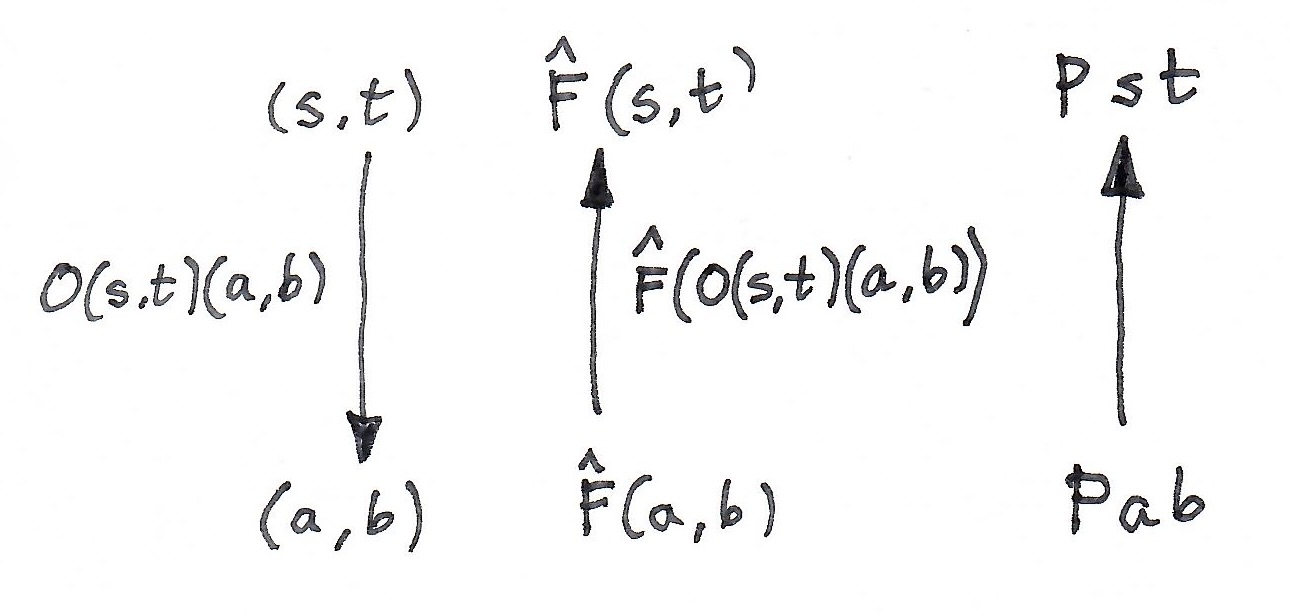
Previously: Kan Extensions in Double Categories.

In programming, actegories play a central role in optics: lenses, prisms, traversals, etc. To understand actegories, let’s start with the definition of a monoidal category.

Monoidal Category

A monoidal category $\mathbf M$ is a category equipped with a tensor product. A tensor product is a functor $\otimes \colon \mathbf M \times \mathbf M \to \mathbf M$ . We assume that this product is associative and unital– up to isomorphism. It means that there is an invertible associator:

$\alpha_{a, b, c} \colon (a \otimes b) \otimes c \to a \otimes (b \otimes c)$

natural in all three arguments. We also have a unit object $1$ and two (invertible, natural) unitors:

$\lambda_a \colon 1 \otimes a \to a$

$\rho_a \colon a \otimes 1 \to a$

To get a better feel for it, we can try to model a monoidal category in Haskell. We parameterize it by the type of the tensor product, ten, which we want to be a Bifunctor:

class (Bifunctor ten) => MonoidalCategory ten where ...

The standard way to define a subcategory of Hask is to restrict the types of objects by imposing a constraint. Such a restriction has a special kind, Constraint:

			
class Bifunctor ten
  => MonoidalCategory (obj :: Type -> Constraint) ten where ...

A common example of such a constraint is a typeclass. For instance Monoid will restrict the objects of the category to be monoids. (In principle, we should also restrict the type of arrows, here to monoid morphisms.)

We can specify the unit of a monoidal category as an associated type (parameterized by ten):

    type Unit ten :: Type

The unit should be an object of the category, so it should satisfy the constraint. We can encode this in our definition as a precondition: obj (Unit ten). This leads to a circularity, which we can overcome using the language pragma UndecidableSuperClasses:

			
class (Bifunctor ten , obj (Unit ten))
  => MonoidalCategory (obj :: Type -> Constraint) ten where
    type Unit ten :: Type
    ...

Finally, we can add the associator and the unitors (and their inverses):

			
class (Bifunctor ten , obj (Unit ten))
  => MonoidalCategory (obj :: Type -> Constraint) ten where
    type Unit ten :: Type
    alpha  :: (obj a, obj b, obj c) =>  (a `ten` b) `ten` c -> a `ten` (b `ten` c)
    lambda :: (obj a) => (Unit ten) `ten` a -> a
    ...

		

Notice the obj constraints in the type of these functions and the infix notation for the tensor.

Let’s work out a few examples. The simplest is the category of all types with a cartesian product as tensor.

			
instance MonoidalCategory Hask (,) where
    type Unit (,) = ()
    alpha ((a, b), c) = (a, (b, c))
    lambda ((), a) = a
    ...

		

We define Hask using an empty class, and we make all objects its instances:

			
class Hask a
instance Hask a

Similarly, we can define a monoidal category with Either as the tensor product, or with Monoid as the object constraint.

Actegory

An actegory is a category that supports the action of a monoidal category. You may think of it as “multiplying” or “scaling” the objects of this category by objects of the monoidal category. The (left) action can be defined as a functor from the product category to $C$ :

$\triangleright \colon \mathbf M \times C \to C$

or, after currying, as a functor from $\mathbf M$ to the endofunctor category:

$\triangleright \colon \mathbf M \to [C, C]$

The coherency conditions are the invertible natural transformations that relate the action $\triangleright$ to the tensor product $\otimes$ and its unit $1$ :

$\alpha_{m n a} \colon (m \otimes n) \triangleright a \to m \triangleright (n \triangleright a)$

$\lambda_{a} \colon 1 \triangleright a \to a$

The action is functorial in both arguments, so our Haskell translation pegs it, for simplicity, as a Bifunctor. (A Profunctor action is also possible. Categorically, it would correspond to using $\mathbf M^{op}$ as the monoidal category.)

			
class (MonoidalCategory obj ten, Bifunctor act) 
  => Actegory obj ten act | act -> ten where
    assoc  :: (obj m, obj n) 
           => (m `ten` n) `act` a -> m `act` (n `act` a)
    assoc' :: (obj m, obj n)
           => m `act` (n `act` a) -> (m `ten` n) `act` a
    unit   :: Unit ten `act` a -> a
    unit'  :: a -> Unit ten `act` a

		

Another simplifying assumption is that the action uniquely identifies the tensor product, encoded here as the functional dependency act -> ten.

The simplest example of an actegory is the self action of the cartesian product. Here, the monoidal category acts on itself:

			
instance Actegory Hask (,) (,) where
    assoc ((m, n), a) = (m, (n, a))
    assoc' (m, (n, a)) = ((m, n), a)
    unit ((), a) = a
    unit' a = ((), a)

		

Monoidal Functors

Actegories that use the same monoidal category for their actions form a category. The morphisms in this category are (strict) monoidal functors. These are functors that map one action to another:

$f (m \triangleright_1 a) \cong m \triangleright _2 f a$

In Haskell, we can model them as:

			
class (Actegory obj ten act1, Actegory obj ten act2, Functor f) =>
  MonFunctor obj ten act1 act2 f where
    as  :: obj m => m `act2` f a   -> f (m `act1` a)
    as' :: obj m => f (m `act1` a) -> m `act2` f a

In fact, actegories form a bicategory, with action-preserving natural transformations acting between monoidal functors.

Here’s an interesting example of a monoidal functor between non-trivial actegories:

			
instance (Traversable f) => MonFunctor Monoid (,) (,) (,) f where
    as (m, fa) = fmap (m, ) fa
    as' = sequenceA

Haskell code is available here.

June 8, 2026

Kan Extensions in Haskell

Posted by Bartosz Milewski under Category Theory, Haskell, Programming | Tags: Category Theory, Haskell, Kan extensions, Universal Arrows |
1 Comment

Previously: Tabulation Tribulations.

If you think of functor composition as a form of multiplication, Kan extensions are an attempt to construct inverses of this multiplication. But unlike multiplication, composition is not symmetric, so we have extensions that attempt to undo precomposition, and lifts that do the same for postcomposition. Furthermore, there rarely is a single inverse to any form of composition, so we have the parsimonious right extensions and lifts, and the generous left extensions and lifts. We end up with four combinations that correspond to four different adjunctions:

$(- \circ j) \dashv \text{Ran}_j -$

$\text{Lan}_j - \dashv (- \circ j )$

$(j \circ -) \dashv \text{Rift}_j -$

$\text{Lift}_j - \dashv (j \circ -)$

We’ll concentrate on the extensions, since we can provide explicit point-wise formulas for them in cases that are of interest to us, that is in $\mathbf{Cat}$ and in $\mathbb{P}rof$ .

Right Kan extensions

The definition of the right Kan extension relates the mapping out of the composition to the mapping into $\text{Ran}$ . In Haskell, we can define them as two types:

			
type Phi  j s d = Compose s j ~> d
type Phi' j s d = s ~> Ran j d

The wavy arrows denote natural transformations:

type f ~> g = forall x. f x -> g x

To show that there is an adjunction we can either prove the (natural) isomorphism between Phi and Phi', or implement the unit and counit of the adjunction (together with zigzag identities):

			
eta     :: (Functor j, Functor d) => d ~> Ran j (Compose d j)
epsilon :: (Functor j, Functor d) => Compose (Ran j d) j ~> d

In Haskell we can implement the right Kan extension as:

newtype Ran j d a = Ran (forall x . (a -> j x) -> d x)

This is a straightforward translation of the categorical formula that uses an end:

$(\text{Ran}_j d) \,a = \int_x \text{Set}(C(a, j \,x), d \, x)$

The adjunction can then be implemented as a pair of mappings:

			
leftAdj :: (Functor j, Functor d, Functor s) =>
   Phi j s d -> Phi' j s d
leftAdj phi sx = Ran (\x_jx -> phi (Compose (fmap x_jx sx)))
rightAdj ::  (Functor j, Functor d, Functor s) =>
   Phi' j s d -> Phi j s d
rightAdj phi' (Compose sj) = 
    let (Ran ran) = phi' sj
    in ran id

		

Or as the unit/counit pair:

			
eta :: (Functor j, Functor d) => d ~> Ran j (Compose d j)
eta dx = Ran (\x_jx -> Compose (fmap x_jx dx))
epsilon :: (Functor j, Functor d) => Compose (Ran j d) j ~> d
epsilon (Compose (Ran ran)) = ran id

Universal arrows

There is a third way, which gives a better starting point for generalizations. It can be used on an object-by-object basis, even if there is no global adjunction. It’s based on the idea of the universal arrow.

A universal arrow is a terminal object in the comma category. For a given functor $L \colon D \to C$ , the comma category $L/c$ consists of pairs $(d, f \colon L d \to c)$ . In other words, it’s a category of arrows from the image of $L$ to some fixed object $c \in C$ . Morphisms in the comma category are arrows $h: d \to d'$ in $D$ that make the corresponding triangles in $C$ commute:

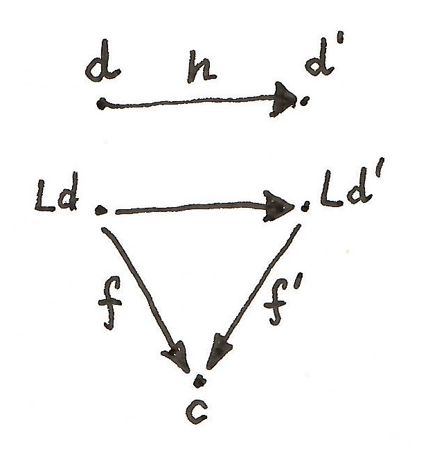
A terminal object in $L/c$ is a pair $(t, \tau)$ , through which every arrow $\Phi \colon L d \to c$ factorizes uniquely. That means, there is a unique arrow $h \colon d \to t$ that makes the following triangle commute:

If there is an adjunction $L \dashv R$ , then we can easily construct the universal arrow as a pair $(R c, \epsilon_c)$ , where $\epsilon_c$ is a component of the counit of the adjunction. Indeed, every $\Phi \colon L d \to c$ factorizes through $\epsilon_c$ :

$\Phi = \epsilon_c \circ L \Phi'$

where $\Phi' = \text{leftAdj}\, \Phi$ .

The advantage of the universal arrow approach is that it’s pointwise. We can do it for each object $c$ separately.

Reversing this process, rather than building an adjuncion, we can directly construct a universal arrow. We start by defining of a component of a counit. Then we postulate that any other counit-like mapping factorizes uniquely throught that counit.

Let’s see how it works for our definition of the right Kan extension. The counit has the following signature:

epsilon :: (Functor j, Functor d) => Compose (Ran j d) j ~> d

We can illustrate it with the following string diagram:

In general, the functors go between three different categories: A, B, and M. In Haskell we have just one category and three endofunctors.

Any other mapping of this form has the signature (replacing Ran j d with an arbitrary functor s):

type Phi j s d = Compose s j ~> d

Or, as a string diagram:

We postulate that, for every Phi, there is a unique Phi' that factorizes it through epsilon. That is, we have a function:

			
leftAdj :: (Functor j, Functor d, Functor s) =>
   Phi j s d -> Phi' j s d

such that:

			
factor :: (Functor j, Functor d, Functor s) => Phi j s d -> Phi j s d
factor phi = epsilon . Compose . leftAdj phi . getCompose

Modulo newtype shenanigans, this is exactly $\epsilon \circ (L_j \Phi')$ , where $L_j s = s \circ j$ is functor precomposition. Or as a string diagram:

Notice that rightAdj doesn’t appear anywhere in this construction.

The computational interpretation of this universal construction lets us calculate a mapping into a right Kan extension. Namely, to determine a natural transformation from some functor s to Ran j d, it’s enough to provide a mapping phi from Compose s j to d.

Left Kan extensions

We can now apply the same idea to the left Kan extension. This time we start with the unit:

eta :: (Functor j, Functor d) => d ~> Compose (Lan j d) j

We postulate that for any other mapping of this form (replacing Lan j d with and arbitrary s):

type Phi j s d = d ~> Compose s j

there is a unique Phi':

type Phi' j s d = Lan j d ~> s

that factorizes it through eta:

			
factor :: (Functor j, Functor d, Functor s) => Phi j s d -> Phi j s d
factor phi = Compose . rightAdj phi . getCompose . eta

In Haskell, the left Kan extension is given by the existential data type:

			
data Lan j d a where
    Lan :: (j x -> a) -> d x -> Lan j d a

In category theory, this formula uses a coend:

$(\text{Lan}_j d) \, a = \int^x C(j \, x, a) \times d \, x$

Indeed, for any given Phi, we can obtain a Phi' by applying this function:

			
rightAdj :: (Functor j, Functor d, Functor s) =>
   Phi j s d -> Phi' j s d
rightAdj d_sj (Lan jx_a dx) = 
    let Compose sjx = d_sj dx
    in fmap jx_a sjx

		

The result factorizes Phi through eta:

			
factor :: (Functor j, Functor d, Functor s) => Phi j s d -> Phi j s d
factor phi = Compose . rightAdj phi . getCompose . eta

The computational interpretation of this universal construction let us calculate a mapping out of the left Kan extension.

See Haskell code for right and left Kan extensions.

Next, we’ll generalize these construction to a double category setting.

May 16, 2026

Profunctor Equipment in Haskell

Posted by Bartosz Milewski under Category Theory, Haskell, Programming | Tags: Category Theory, Haskell, Profunctor Equipment |
[2] Comments

Previously: Profunctor Equipment.

To make things more palatable for programmers, I decided to provide a toy implementation of some of the equipments in Haskell. The advantage of this encoding is that it can be verified by the compiler, and I still trust the compiler more than I trust the AI.

A more adequate implementation would require a full-blown dependently typed language, but if we restrict ourselves to just a single category and work only with endo-functors and endo-profunctors, we can get at least some intuitions. If you want to see a more elaborate version, see the proarrows library by Sjoerd Visscher.

The only 0-cell I’ll be using is the Haskell category of types and functions. For vertical 1-cells I’ll use the standard library implementation of Functor, and for horizontal ones I’ll use Profunctor.

A 2-cell in $\mathbb{P}rof$ :

is implemented as a natural transformation:

type Cell f g h j = forall a c . h a c -> j (f a) (g c)

The forall serves as a universal quantifier.

The horizontal composition of such cells is given by:

hcomp :: (Functor f, Functor f', Functor g, Functor g'
         , Profunctor h, Profunctor j, Profunctor k) =>
    Cell f g h j -> Cell f' g' j k 
                 -> Cell (Compose f' f) (Compose g' g) h k
hcomp fg_hj fg_jk hac = dimap getCompose Compose $ fg_jk (fg_hj hac)

I used the library definition of functor composition:

newtype Compose f g a = Compose { getCompose :: f (g a) }

Vertical composition of cells uses a more elaborate profunctor composition:

vcomp :: (Functor f, Functor g, Functor h
         , Profunctor p, Profunctor q, Profunctor r, Profunctor s) =>
    Cell f g p r -> Cell g h q s 
                 -> Cell f h (Procompose q p) (Procompose s r)
vcomp fg_pr gh_qs (Procompose qxc pax) 
    = Procompose (gh_qs qxc) (fg_pr pax)

Profunctor composition is defined using a coend. In Haskell, we implement a coend:

$\int^x P \langle x, c\rangle \times Q \langle d, x \rangle$

as an existential type:

data Procompose p q d c where
  Procompose :: p x c -> q d x -> Procompose p q d c

Here, x is a type that’s not in the argument list, so it’s interpreted using the existential counterpart of forall.

This is the horizontal unit cell:

type Hunit p = Cell Identity Identity p p

hUnit :: Profunctor p => Hunit p
hUnit = dimap runIdentity Identity

and here’s its vertical counterpart:

type Vunit f a b = Cell f f (->) (->)

vUnit :: Functor f => Vunit f a b
vUnit = fmap

I used the library implementation of the Identity functor, and the type constructor (->) for the hom-profunctor–the unit of profunctor composition. The unit laws are satisfied up to isomorphism.

The companion and the conjoint are synonyms of the library types Costar and Star:

newtype Star f d c   = Star   { runStar   :: d -> f c }
newtype Costar f d c = Costar { runCostar :: f d -> c }

type Companion f d c = Costar f d c
type Conjoint f d c  = Star f d c

The companion unit and counit cells:

are given by, respectively:

type CompUnit f   = Cell Identity f (->) (Costar f)

compUnit :: Functor f => CompUnit f
compUnit h = Costar (fmap (h . runIdentity))

and

type CompCoUnit f = Cell f Identity (Costar f) (->)

compCoUnit :: Functor f => CompCoUnit f 
compCoUnit (Costar h) = Identity . h

Similarly for the conjoint:

type ConjUnit f   = Cell f Identity (->) (Star f)

conjUnit :: Functor f => ConjUnit f 
conjUnit h = Star  (fmap (Identity . h))

and:

type ConjCoUnit f = Cell Identity f (Star f) (->)

conjCoUnit :: Functor f => ConjCoUnit f 
conjCoUnit (Star h) = h . runIdentity

More advanced constructions would require the definition of categories internal to Hask and the use of dependent types.

Haskell code is available here.

January 4, 2025

Legalizing Comonad Composition

Posted by Bartosz Milewski under Category Theory, Haskell, Programming | Tags: Category Theory, Comonad, Game of Life, Haskell |
[7] Comments

The yearly Advent of Code is always a source of interesting coding challenges. You can often solve them the easy way, or spend days trying to solve them “the right way.” I personally prefer the latter. This year I decided to do some yak shaving with a puzzle that involved looking for patterns in a grid. The pattern was the string XMAS, and it could start at any location and go in any direction whatsoever.

My immediate impulse was to elevate the grid to a comonad. The idea is that a comonad describes a data structure in which every location is a center of some neighborhood, and it lets you apply an algorithm to all neighborhoods in one fell swoop. Common examples of comonads are infinite streams and infinite grids.

Why would anyone use an infinite grid to solve a problem on a finite grid? Imagine you’re walking through a neighborhood. At every step you may hit the boundary of a grid. So a function that retrieves the current state is allowed to fail. You may implement it as returning a Maybe value. So why not pre-fill the infinite grid with Maybe values, padding it with Nothing outside of bounds. This might sound crazy, but in a lazy language it makes perfect sense to trade code for data.

I won’t bore you with the details, they are available at my GitHub repository. Instead, I will discuss a similar program, one that I worked out some time ago, but wasn’t satisfied with the solution: the famous Conway’s Game of Life. This one actually uses an infinite grid, and I did implement it previously using a comonad. But this time I was more ambitious: I wanted to generate this two-dimensional comonad by composing a pair of one-dimensional ones.

The idea is simple. Each row of the grid is an infinite bidirectional stream. Since it has a specific “current position,” we’ll call it a cursor. Such a cursor can be easily made into a comonad. You can extract the current value; and you can duplicate a cursor by creating a cursor of cursors, each shifted by the appropriate offset (increasing in one direction, decreasing in the other).

A two-dimensional grid can then be implemented as a cursor of cursors–the inner one extending horizontally, and the outer one vertically.

It should be a piece of cake to define a comonad instance for it: extract should be a composition of (extract . extract) and duplicate a composition of (duplicate . fmap duplicate), right? It typechecks, so it must be right. But, just in case, like every good Haskell programmer, I decided to check the comonad laws. There are three of them:

extract . duplicate = id
fmap extract . duplicate = id
duplicate . duplicate = fmap duplicate . duplicate

And they failed! I must have done something illegal, but what?

In cases like this, it’s best to turn to basics–which means category theory. Compared to Haskell, category theory is much less verbose. A comonad is a functor $W$ equipped with two natural transformations:

$\varepsilon \colon W \to \text{Id}$

$\delta \colon W \to W \circ W$

In Haskell, we write the components of these transformations as:

extract :: w a -> a
duplicate :: w a -> w (w a)

The comonad laws are illustrated by the following commuting diagrams. Here are the two counit laws:

and one associativity law:

These are the same laws we’ve seen above, but the categorical notation makes them look more symmetric.

So the problem is: Given a comonad $W$ , is the composition $W \circ W$ also a comonad? Can we implement the two natural transformations for it?

$\varepsilon_c \colon W \circ W \to \text{Id}$

$\delta_c \colon W \circ W \to W \circ W \circ W \circ W$

The straightforward implementation would be:

$W \circ W \xrightarrow{\varepsilon \circ W} W \xrightarrow{\varepsilon} \text{Id}$

corresponding to (extract . extract), and:

$W \circ W \xrightarrow{W \circ \delta} W \circ W \circ W \xrightarrow{\delta \circ W \circ W} W \circ W \circ W \circ W$

corresponding to (duplicate . fmap duplicate).

To see why this doesn’t work, let’s ask a more general question: When is a composition of two comonads, say $W_2 \circ W_1$ , again a comonad? We can easily define a counit:

$W_2 \circ W_1 \xrightarrow{\varepsilon_2 \circ W_1} W \xrightarrow{\varepsilon_1} \text{Id}$

The comultiplication, though, is tricky:

$W_2 \circ W_1 \xrightarrow{W_2 \circ \delta_1} W_2 \circ W_1 \circ W_1 \xrightarrow{\delta_2 \circ W} W_2 \circ W_2 \circ W_1 \circ W_1$

Do you see the problem? The result is $W_2^2 \circ W_1^2$ but it should be $(W_2 \circ W_1)^2$ . To make it a comonad, we have to be able to push $W_2$ through $W_1$ in the middle. We need $W_2$ to distribute over $W_1$ through a natural transformation:

$\lambda \colon W_2 \circ W_1 \to W_1 \circ W_2$

But isn’t that only relevant when we compose two different comonads–surely any functor distributes over itself! And there’s the rub: Not every comonad distributes over itself. Because a distributive comonad must preserve the comonad laws. In particular, to restore the the counit law we need this diagram to commute:

and for the comultiplication law, we require:

Even if the two comonad are the same, the counit condition is still non-trivial:

The two whiskerings of $\varepsilon$ are in general not equal. All we can get from the original comonad laws is that they are only equal when applied to the result of comultiplication:

$(\varepsilon \circ W) \cdot \delta = (W \circ \varepsilon) \cdot \delta$ .

Equipped with the distributive mapping $\lambda$ we can complete our definition of comultiplication for a composition of two comonads:

$W_2 \circ W_1 \xrightarrow{W_2 \circ \delta_1} W_2 \circ W_1^2 \xrightarrow{\delta_2 \circ W} W_2^2 \circ W_1^2 \xrightarrow{W_2 \circ \lambda \circ W_1} (W_2 \circ W_1)^2$

Going back to our Haskell code, we need to impose the distributivity condition on our comonad. There is a type class for it defined in Data.Distributive:

class Functor w => Distributive w where
  distribute :: Functor f => f (w a) -> w (f a)

Thus the general formula for composing two comonads is:

instance (Comonad w2, Comonad w1, Distributive w1) => 
  Comonad (Compose w2 w1) where
    extract = extract . extract . getCompose
    duplicate = fmap Compose . Compose .
                fmap distribute . duplicate . fmap duplicate .
                getCompose

In particular, it works for composing a comonad with itself, as long as the comonad distributes over itself.

Equipped with these new tools, let’s go back to implementing a two-dimensional infinite grid. We start with an infinite stream:

data Stream a = (:>) { headS :: a
                     , tailS :: Stream a}
  deriving Functor

infixr 5 :>

What does it mean for a stream to be distributive? It means that we can transpose a “matrix” whose rows are streams. The functor f is used to organize these rows. It could, for instance, be a list functor, in which case you’d have a list of (infinite) streams.

  [   1 :>   2 :>   3 .. 
  ,  10 :>  20 :>  30 ..
  , 100 :> 200 :> 300 .. 
  ]

Transposing a list of streams means creating a stream of lists. The first row is a list of heads of all the streams, the second row is a list of second elements of all the streams, and so on.

  [1, 10, 100] :>
  [2, 20, 200] :>
  [3, 30, 300] :>
  ..

Because streams are infinite, we end up with an infinite stream of lists. For a general functor, we use a recursive formula:

instance Distributive Stream where
    distribute :: Functor f => f (Stream a) -> Stream (f a)
    distribute stms = (headS  stms) :> distribute (tailS  stms)

(Notice that, if we wanted to transpose a list of lists, this procedure would fail. Interestingly, the list monad is not distributive. We really need either fixed size or infinity in the picture.)

We can build a cursor from two streams, one going backward to infinity, and one going forward to infinity. The head of the forward stream will serve as our “current position.”

data Cursor a = Cur { bwStm :: Stream a
                    , fwStm :: Stream a }
  deriving Functor

Because streams are distributive, so are cursors. We just flip them about the diagonal:

instance Distributive Cursor where
    distribute :: Functor f => f (Cursor a) -> Cursor (f a)
    distribute fCur = Cur (distribute (bwStm  fCur)) 
                          (distribute (fwStm  fCur))

A cursor is also a comonad:

instance Comonad Cursor where
  extract (Cur _ (a :> _)) = a
  duplicate bi = Cur (iterateS moveBwd (moveBwd bi)) 
                     (iterateS moveFwd bi)

duplicate creates a cursor of cursors that are progressively shifted backward and forward. The forward shift is implemented as:

moveFwd :: Cursor a -> Cursor a
moveFwd (Cur bw (a :> as)) = Cur (a :> bw) as

and similarly for the backward shift.

Finally, the grid is defined as a cursor of cursors:

type Grid a = Compose Cursor Cursor a

And because Cursor is a distributive comonad, Grid is automatically a lawful comonad. We can now use the comonadic extend to advance the state of the whole grid:

generations :: Grid Cell -> [Grid Cell]
generations = iterate $ extend nextGen

using a local function:

nextGen :: Grid Cell -> Cell
nextGen grid
  | cnt == 3 = Full
  | cnt == 2 = extract grid
  | otherwise = Empty
  where
      cnt = countNeighbors grid

You can find the full implementation of the Game of Life and the solution of the Advent of Code puzzle, both using comonad composition, on my GitHub.

July 16, 2012

The Functor Pattern in C++

Posted by Bartosz Milewski under Programming | Tags: C++11, functor, Haskell, Programming, templates |
Leave a Comment

The post is on the FP Complete site. Time to graduate from the GoF patterns into something a bit more abstract. Have fun!

[twitter-follow screen_name=’BartoszMilewski’]

Bartosz Milewski's Programming Cafe

Actegories

Monoidal Category

Actegory

Monoidal Functors

Kan Extensions in Haskell

Right Kan extensions

Universal arrows

Left Kan extensions

Profunctor Equipment in Haskell

Legalizing Comonad Composition

The Functor Pattern in C++

Top Posts

License

Blogroll

Follow Me

Archives