Haskell

Archived Posts from this Category

July 15, 2014

Natural Transformations and Ends

Posted by Bartosz Milewski under Category Theory, Haskell
[3] Comments

In category theory we never look inside objects. All information about objects is encoded in the arrows (morphisms) between them. In set theory, on the other hand, we express properties of sets through their elements. But there is a strong link between categories and sets, at least in the case of locally small categories. In those categories, morphisms between any two objects form a set. We call this set the hom-set.

Go one level up in abstraction and you have categories of functors, which are mappings between categories. In a functor category a functor is treated as an object, and a natural transformation — a mapping between functors– is treated as a morphism. So a hom-set in a functor category is a set of natural transformations between two functors. An interesting question arises: How is this set related to the hom-sets in the categories that are mapped by these functors? After all, they are sets in the same category of sets. The answer involves, as usual, a universal construction. This one is called an end.

Notation

The problem with category theory is that it deals with so many levels of abstraction that you quickly run out of fonts for your notation. I’ll try to stick to more or less the standard notation. I’ll use capital letters C, D, etc. for categories (script font would be nice, but it’s not very practical in a blog). The corresponding lower case letters, c, d — optionally with primes, like c', d' — will denote objects in those categories. I’ll use f, g, h, etc. for morphisms and F, G, H for functors. I’ll also use the terse notation for hom-sets, so the set of all morphisms between objects c and c' in category C will be simply C(c, c'). The set of natural transformations between two functors F and G, both mapping C to D, will be [C, D](F, G). I will not use parentheses for functors acting on objects or morphisms, so F acting on c will be simply F c (and similarly F f, when acting on f). But occasionally I’ll break the rules if it helps the presentation.

Natural Transformations

A natural transformation is a map between functors. So let’s start with two functors F and G, both going from category C to another category D. Let’s focus on one object in C, call it c. F maps c to F c and G maps c to G c. These two, F c and G c, are objects in D. As such they define a hom-set: the set of all morphisms from F c to G c denoted D(F c, G c). A natural transformation picks one morphism from every such hom-set. Not all picks are natural, as we’ll see soon.

Hom-set defined by two images of object c under functors F and G

A hom-set, being a set, is also an object in Set — the category of sets. So let’s look at the hom-sets D(F c, G c) as objects in Set. There is one for every c. If we carefully pick one element from each, we will have a natural transformation (I said “carefully”). A natural transformation is a family of morphisms picked from hom-sets D(F c, G c), one for each c. If you think of those hom-sets as fibers growing from objects in C, a natural transformation is a cross-section through all these fibers.

Here’s another way of looking at this. Let’s pick an arbitrary set in Set, call it X (sorry, I’m using a capital letter for an object in Set, but I do need lowercase x for its element). A function φ from X to the set D(F c, G c) maps an element x of X to a particular morphism in D(F c, G c). We can think of it as picking a component of some natural transformation. Each choice of x would potentially correspond to a different natural transformation. So the set X could be looked upon as representing some set of natural transformations. We still have to fill in a lot of blanks, but we are on the right track.

A function from a set X to a hom-set defined by two functors F and G

Since a natural transformation is a family of morphisms, we need a family of such functions from X to D(F c, G c), one for every c. Let’s call this family τ. When we fix c, it’s a function from X to D(F c, G c). When we fix x, it’s a precursor of a natural transformation: a family of morphisms picked from hom-sets.

A family of functions parameterized by c and x

The only thing missing from this picture is the naturality condition. Not all families of D(F c, G c) are natural. We need to account for the fact that our functors F and G not only map objects, but also morphisms.

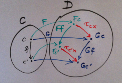
So let’s look at morphisms in C and how they are mapped to morphisms in D by, say, our functor F. We can pick two object in C, c and c'. Morphisms between those two form a hom-set C(c, c'). F maps this hom-set to another hom-set, D(F c, F c'). Similarly, G maps the same hom-set to D(G c, G c').

Four hom-sets defined by two functors F and G and two objects c and c’. A natural transformation is a recipe for picking red arrows.

Taken together, we have a diagram of four hom-sets between four objects: F c, F c', G c, and G c'. Fixing a morphism f from c to c' (an element of C(c, c')) picks two morphisms, one F f from D(F c, F c') and one G f from D(G c, G c'), given the functoriality of F and G. Fixing an x in X picks two morphisms, one τ_{c x} from D(F c, G c) and one τ_{c' x} from D(F c', G c'). These four better commute:

G f . τ_{c x} = τ_{c' x} . F f

The commuting naturality square

That’s the naturality condition. Any τ that satisfies this condition defines a set of natural transformations, one for each x.

Wedges

All this time I’ve been setting up the scene for one important insight. The set X and the family of functions τ look a lot like a cone (see my blog post about limits). Except that, instead on one functor, we have two, and τ is not really a natural transformation. But we are getting close. And if we can carve out something cone-like out of this construction, than we could maybe find something limit-like. And indeed the cone-like object is called a wedge and the limit-like thing is called an end, and in our case the end would be a set of all natural transformations from F to G. So let’s work this thing out.

If we were constructing a cone, we’d start with a functor from our source category C to the target category — Set in this case. That’s easy to define for objects: c goes into the set D(F c, G c). But we run into a problem with morphisms. Suppose we want to map a morphism h that goes from c to c':

h : c -> c'

Its image should be a function from D(F c, G c) to D(F c', G c'). It’s a function that maps morphisms to morphisms. Let’s see what morphisms are at our disposal. We have:

F h : F c -> F c'
G h : G c -> G c'

How can we turn a morphism f from D(F c, G c)

f : F c -> G c

into a morphism f' from D(F c', G c'):

f' : F c' -> G c'

One thing we could do is to post-compose G h after f to get to G c'; but there is no way to get anywhere from F c'. So it can’t be that simple.

But notice one thing. Even though τ maps elements of X to “diagonal” hom-sets (by diagonal I mean that the argument c is repeated in D(F c, G c)), naturality condition involves off-diagonal hom-sets, like D(F c, F c') and D(G c, G c') (c potentially different from c'). So maybe we should open our minds to those off-diagonal hom-sets in our search of a functor? How about a functor that maps a pair of elements (c, c') to a hom-set D(F c, G c')? Let’s see if we can figure out its action on morphisms.

Now, since we are constructing a functor of two arguments, we have to define its action on a pair of morphisms, (f, g).

f : c -> c'
g : d -> d'

The image of this pair should be a function in Set that maps D(F c, G d) into D(F c', G d'). Unfortunately, we run into the same problem again. Given h : F c -> G d, we can follow it with G g : G d -> G d', but there is no way we can move anywhere from F c'. The only morphism at our disposal goes the wrong way, F f : F c -> F c'. If we could only reverse it!

Ah! but functors that go “the wrong way” on morphisms are well known. They are called contravariant functors, as opposed to the good old covariant functors that we have grown to love and cherish. What we need is a functor that’s contravariant in the first argument and covariant in the second. Such functors even have a name: they are called profunctors.

So, given a pair of morphisms (f, g) our profunctor S_nat will map a morphism from D(F c', G d) to a morphism from D(F c, G d'). Notice that this time I have inverted c and c'.

Given h : F c' -> G d, we can easily construct a correpsponding morphism in D(F c, G d') by this composition:

G g . h . F f : F c' -> G d

Constructing the action of a profunctor built from two functors on a pair of morphisms

So that’s our action of S_nat on a pair of morphisms from C. It turns a morphism h into:

(S_nat f g) h = G g . h . F f

Let’s summarize what we have so far: We have a profunctor S_nat, a set X, and a family of morphisms τ from X to diagonal elements S_nat c c. We are not interested in defining τ for off-diagonal elements of S_nat. What remains is to impose some kind of generic condition on τ that would let it generate natural transformations only. We would like to formulate this condition in terms of a general profunctor S, if possible.

What’s the minimal consistency condition on τ, given that it only generates diagonal elements S c c? We need a way to somehow connect two such objects, say S c c and S c' c'. Suppose we have a morphism f : c -> c'. How can we use this morphism to operate on S c c and S c' c'? A profunctor S can be used to map a pair of morphisms, so how about pairing our f with something obvious that always exists, like the identity morphism id? Let’s try it:

S id_c f  : S c  c  -> S c c'
S f id_c' : S c' c' -> S c c'

(Notice the inversion of c and c' when f is used as the first argument — that’s our contravariance in action.) We have found two ways to get from two diagonal elements to the same non-diagonal element of S. Together with τ_c and τ_c' they form a diamond. This diamond better commute or we’re in trouble.

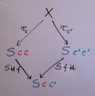
The wedge condition

S id_c f . τ_c = S f id_c' . τ_c'

Now we can finally define a wedge for an arbitrary profunctor S. A wedge for S consists of an object X and a family of morphisms τ_c from X to S c c that satisfy the wedge condition above.

And if we plug in our special profunctor S_nat that maps pairs of objects to hom-sets, the wedge condition turns into the naturality condition for our two functors. Let’s check this out.

Remember, this is how S_nat acts on a pair of morphisms f and g:

(S_nat f g) h = G g . h . F f

Substituting identities in the right places, we get (remember, functors turn identities into identities):

(S_nat id_c f) h = G f . h
(S_nat f id_c') h' = h' . F f

Notice that h and h' are morphisms in D but, at the same time, elements of sets S c c and S c' c' in the wedge condition. They are given, respectively, by the action of τ_c and τ_c’ on an element x of X. The wedge condition for S_nat will therefore post-compose τ_c and pre-compose τ_c:

G f . τ_c = τ_c' . F f

And this is exactly the naturality condition for components of τ. It means that τ that satisfies the wedge condition is a natural transformation for any choice of x.

Dinatural transformations

This definition of a wedge looks almost like the definition of a cone, except that the commuting conditions in a cone were expressed in terms of naturality of the transformation between the diagonal functor Δ_X and the functor F. Here, we could also say that the object X is an image of a diagonal profunctor Δ_X — trivially defined to map pairs of objects from C to an object X, and pairs of morphisms to the identity morphism on X.

A wedge (Strictly speaking, a profunctor is a mapping from C^opxC to D — the “op” accounting for the reversal of the direction of morphisms in the first argument)

So what we need to complete the picture is some generalized notion of a natural transformation between two profunctors R and S. Since we are only interested in the mapping of diagonal elements of profunctors, this transformation will be called a dinatural transformation (diagonally natural). All we need is to expand the top vertex of the diamond diagram (the wedge condition) to create the commuting hexagon below.

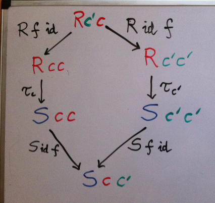
Dinaturality condition

S id_c f . τ_c . R f id_c = S f id_c' . τ_c' . R id_c' f

With this dinaturality condition we can define a wedge for any profunctor S with a vertex X as a dinatural transformation between Δ_X and S.

Now, just as we have defined a limit as a universal cone, we can define an end as a universal wedge. An end is an object End S and a dinatural transformation ω such that for any other wedge (X, τ) there is a unique morphism h from X to End S for which all the triangles in the following diagram commute:

The end as a universal wedge

In particular, since the wedges for our profunctor S_nat defined natural transformations, their end defines the set of all natural transformations between the functors F and G: [C, D](F, G).

There is special notation for an end using the integral symbol. We are “integrating” a profunctor S along a diagnonal over all objects c in category C.

End S = ∫ _c S(c, c)

Using this notation, the set of natural transformations can be written as the following end:

[C, D](F, G) = ∫ _c D(F c, G c)

Note: This is a bit of abuse of notation that happens quite often in category theory. The integral sign makes more sense for coends, which are duals of ends. Coends are related to colimits, which include coproducts, which are the category theory proxies for sums. In this sense, a coend is a generalization of a sum; just as an integral is an infinite continuous sum. By the same token, an end is a generalization of a product. Unfortunately, there is no common symbol for a continuous product in calculus, so we are stuck with the integral symbol.

In Haskell, ends become universal quantifiers, hence this definition of natural transformation from Edward Kmett’s category extras (here f and g are functors):

type f :~> g = forall a. f a -> g a
type Natural f g = f :~> g

You can find more about representing profunctors, dinatural transformations, and ends in Haskell in Edward’s blog.

The Moment of Zen

You can think of a hom-set as defining a mapping: It takes a pair of objects and generates a set of morphisms — an object in Set. A profunctor generalizes this idea. It takes a pair of objects and generates a hom-set-like object in a category that’s not necessarily the category of sets. The mapping from a pair of objects to a hom-set is functorial: its action on pairs of morphisms is well defined as well. Except that this action is contravariant in the first argument and covariant in the second. And so is a profunctor which imitates it.

We’ve seen before how a functor can embed a simple graph into a category and define a limit. The limit embodies the structure of this graph in a single object. A profunctor embeds a structure of a hom-set into a category. An end then embodies this structure in a single object. When this hom-set structure is fashioned using two functors, the end becomes a set of mappings between those two functors — a set of natural transformations. But nothing stops us from fashioning more complex hom-set-like structures and finding their ends.

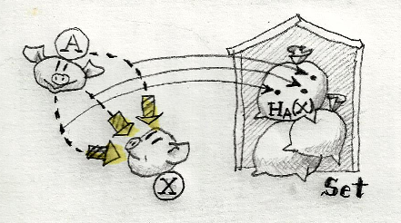
One such construction I’ve had my eyes on for a long itme is called the Kan extension. To give you an idea, imagine a functor T that’s defined on a sub-category M of a bigger category C. It maps it into a category A. The question is, can we extend, or interpolate, this functor over the rest of C? How would we define its value on an object c that’s not in M? The trick is to look at all the hom-sets that go from c to objects in M.

Kan extension setup

Our extended functor will have to map not only c to an object in A, but also all those hom-sets to hom-sets in A. After all, that’s what functors do. This mapping of hom-sets looks very much like a profunctor. It has to be contravariant in its source and covariant in its target. If this profunctor has an end, that’s a perfect candidate for the image of c under the extended functor. That, in a nutshell, is the idea behind the right Kan extension (the left one is, predictably, built with coends). But that’s a topic for another blog post.

June 17, 2014

Exponentials, Currying, and Universal Constructions

Posted by Bartosz Milewski under Category Theory, Haskell, Programming
[9] Comments

Haskell is a language deeply rooted in category theory. But as you don’t need to study the root system of Vitis vinifera in order to enjoy a glass of wine, you don’t need to know much about category theory in order to program in Haskell. Nevertheless, some of us just can’t help ourselves. We have to dig into the rich terroir of category theory to gain deeper insight into the art of functional programming. And today I’d like to talk about functions.

The basic category-theoretical model for Haskell is the category Hask, where objects are Haskell types, and morphisms are functions. The problem with this picture is that it puts functions on a different footing than the rest of the language. Functions from type A to type B — in other words, morphisms from object A to object B in Hask — form a set. This set is called the hom set, Hom(A, B). The fact that it’s just a set and not something bigger is a property of Hask — the property of being locally small. But in Haskell functions from type A to type B also form a type A->B. A type is an object in Hask. So what’s the connection between the set Hom(A, B) and the object A->B? The answer to this question is very interesting and involves products, exponentials, currying, and of course universal constructions.

In my previous blog I talked about the universal construction of limits — objects that represent relationships between other objects. In particular, a product can be defined as such a limit representing the most trivial relationship between two objects — that of just being two objects. Morphisms are also involved in relationships between objects, so maybe there is a way of representing them as an object as well. And indeed, it’s possible to define an object to represent a set of morphisms between two other objects A and B. Such an object is called the exponential and denoted by B^A.

Notice that the domain A of the morphisms appears in the exponent. That might seem odd at first, but it makes perfect sense if you consider the relationship between multiplication (product) and exponentiation. In arithmetic, mⁿ means m multiplied by itself n times. If you replace m and n with types (for simplicity, think of types as sets of values) and multiplication with (set-theoretical) product, you can think of mⁿ as a set of n-tuples of values of type m: (m₁, m₂, m₃,… m_n). Of course, if n is a type, it’s not immediately clear what an n-tuple is (it’s a categorical power), but you can gain some intuition if you consider enumerated finite types. For instance, functions from Bool to any type m, Bool->m, can be represented as all possible pairs of ms (one value for True and one for False). They correspond to the exponential m^Bool. Also, for finite types, the number of different functions from n to m is equal to mⁿ. But the connection between products and exponentials goes deeper than that.

Universal Construction

The basic relationship describing a function is that of application. Given a pair (function, argument), produce a result. It terms of types, a function of type X->Y applied to X produces Y. We want to define the exponential object Y^X to model this relationship. How do we do that?

There isn’t really that much choice. We need to map a pair of objects (Y^X, X) to Y. But what is a pair, and what does it mean to map? We can represent the pair as an object — a product of Y^X × X — and then we can map it to Y using a morphism, which we’ll call app.

It immediately follows that we can’t define exponential objects if we don’t have products. Again, it kind of make intuitive sense — exponentiation arising from iterated multiplication.

From previous experience we know that having a relationship between objects is usually not enough to define a new object. There may be many other objects that model this relationship. We need a way to compare them and pick the one that models it best.

So suppose that we have an impostor object Z, together with a morphism g from Z × X to Y impersonating application. We know that our choice for Y^X is universal if for any Z and g there is a unique morphism, which we’ll call λg, that maps Z to Y^X, and which factors through app:

g = app . (λg, id)

Universality diagram defining the exponential object

Such universal object might not exist in every category, but it does in Hask. In general, a category in which there is a terminal object, a product of any two objects, and an exponential of any two objects is called Cartesian closed. Cartesian closed categories are, for obvious reasons, very important in computer science.

Currying

There’s another way of looking at the diagram that defines the exponential object. You can think of the morphism g as a function of two variables:

g :: (Z, X) -> Y

For any such g there is a unique morphism λg that maps Z to Y^X, an object representing a function from X to Y. This establishes a one-to-one correspondence between functions of two variables and functions returning functions, which we know under the name of currying. So currying “falls out” of the definition of the exponential object.

Adjunction

Any time there is a one-to-one correspondence between sets of morphisms you might want to look for an underlying adjunction. You might remember from my previous blog post that a functor F is said to be left adjoint to the functor G (or G right adjoint to F) if the following two hom sets are naturally isomorphic:

Hom(FZ, Y) ~ Hom(Z, GY)

In our case we have a one-to-one mapping between the morphism g from Z×X to Y and the morphism λg from Z to Y^X. In a category where all products and all exponentials exist, we can define these two functors:

F_XZ = Z × X
G_XY = Y^X

In Haskell, these functors would be implemented as:

newtype F x z = F (z, x)
instance Functor (F x) where
    fmap f (F (z, x)) = F (f z, x)

newtype G x y = G (x -> y)
instance Functor (G x) where
    fmap f (G g) = G (f . g)

and the isomorphism of hom sets would be given by the function phi and its inverse phi':

phi :: (F x z -> y) -> z -> G x y
phi f z = G $ \x -> f (F (z, x))

phi' :: (z -> G x y) -> F x z -> y
phi' g (F (z, x)) = let G f = g z 
                    in f x

Exponentiation can thus be defined as the right adjoint of taking a product.

January 28, 2014

You Can’t Make an Algebra without Breaking a Few Eggs

Posted by Bartosz Milewski under Category Theory, Functional Programming, Haskell, Monads, Programming
[8] Comments

In my previous post I worked on stretching the intuition of what a container is. I proposed that, in Haskell, any functor may be interpreted as some kind of container, including the hard cases like the state functor or the IO functor. I also talked about natural transformations between functors as “repackaging” schemes for containers, which work without “breaking the eggs” — not looking inside the elements stored in the container. Continuing with this analogy: Algebras are like recipes for making omelets.

The intuition is that an algebra provides a way to combine elements stored inside a container. This cannot be done for arbitrary types because there is no generic notion of “combining.” So an algebra is always defined for a specific type. For instance, you can define an algebra for numbers because you know how to add or multiply them, or for strings because you can concatenate them, and so on. The way elements are combined by an algebra is in general driven by the structure of the container itself.

For example, think of an expression tree as a container.

data Expr a = Const a 
            | Add (Expr a) (Expr a) 
            | Mul (Expr a) (Expr a)

We could define many algebras for it. An integer algebra would work on an expression tree that stores integers. A complex algebra would work on a tree that stores complex numbers. A Boolean algebra would work on Boolean expressions using, for instance, logical OR to evaluate the Add node and logical AND for the Mul node. You could even define an algebra of sets with union and intersection for Add and Mul. In fact, in the absence of any additional requirements, any pair of binary functions acting on a given type will do.

The definition of an algebra for a given functor f consists of a type t called the carrier type and a function called the action. Any Haskell algebra is therefore of the type:

newtype Algebra f t = Algebra (f t -> t)

More abstractly, in category theory, an algebra (or, more precisely, an F-algebra) for an endofunctor F is a pair (A, alg) of an object A and a morphism alg : F A -> A. As always, the standard translation from category theory to Haskell replaces objects with types and morphisms with functions.

Let’s have a look at a simple example of an algebra. Let’s pick the list functor and define an Int algebra for it, for instance:

sumAlg :: Algebra [] Int
sumAlg = Algebra (foldr (+) 0)

Despite its simplicity, this example leads to some interesting observations.

First, the use of foldr tells us that it’s possible to handle recursion separately from evaluation. The evaluation is really parameterized here by the function (+) and the value, zero. The algebra is type-specific. On the other hand, foldr is fully polymorphic. It turns out that there is another algebra hidden in this example, and it’s determined just by (+) and zero. We’ll see that more clearly when we talk about fixed points of functors.

The second observation is that a list is not only a functor but also a monad. Is there something special about algebras for a monad? We’ll see.

Algebras and Fixed Points

I wrote a whole blog post about F-algebras with a more categorical slant. Here I’ll elaborate on the Haskell aspects of algebras and develop some more intuitions.

A recursive container is not only a functor but it can also be defined as a fixed point of a functor. So, really, we should start with a double functor, parameterized by two types, a and b:

data ExprF a b = Const a
               | Add b b
               | Mul b b
     deriving Functor

We can then find its fixed point: a type that, when substituted for b, will give back itself. Think of a functor as a TV camera (sorry for switching metaphors). When you point it at some type b, its image appears in all the little monitors where b is on the right hand side of the definition. We all know what happens when you point the camera back at the monitors — you get the ever receding image within image within image… That’s your fixed point.

This “pointing of the camera at the monitors” can be abstracted into a Haskell data structure. It is parameterized by a functor f, which provides the camera and the monitors. The fixed point is given by the ever receding:

newtype Fix f = In (f (Fix f))

Notice that, on the left hand side, f appears without an argument. If f a is a container of a then f by itself is a recipe for creating a container from any type. Fix takes such a recipe and applies it to itself — to (Fix f).

Later we’ll also need the deconstructor, unIn:

unIn :: Fix f -> f (Fix f)
unIn (In x) = x

Going back to our earlier functor, we can apply Fix to it and get back the recursive version of Expr:

type Expr a = Fix (ExprF a)

Here, (ExprF a) is a recipe for stuffing any type b into a simple (non-recursive) container defined by ExprF.

Creating actual expressions using the above definition of Expr is a little awkward, but possible. Here’s one:

testExpr :: Expr Int
testExpr = In $ (In $ (In $ Const 2) `Add` (In $ Const 3)) 
                `Mul` (In $ Const 4)

Knowing that a recursive data type such as (Expr a) is defined in terms of a simpler functor (ExprF a b) means that any recursive algebra for it can be defined in terms of a simpler algebra. For instance, we can define a simple algebra for (ExprF Int) by picking the carrier type Double and the following action:

alg :: ExprF Int Double -> Double
alg (Const i) = fromIntegral i
alg (Add x y) = x + y
alg (Mul x y) = x * y

We can use this algebra to work on arbitrary recursive expressions of type Expr Int. We’ll call this new recursive function eval. When given an (Expr Int) it will do the following:

Extract the contents of the outer Fix by pattern matching on the consturctor In. The contents is of the type ExprF acting on (Expr Int).
Apply eval (the recursive one we are just defininig) to this contents. Do this using fmap. Here we are taking advantage of the fact that ExprF is a functor. This application of eval replaces the children of the expression ExprF with Doubles — the results of their evaluation.
Apply alg to the result of the previous step, which is of the type (ExprF Int Double).

Here’s the code that implements these steps:

eval :: Fix (ExprF Int) -> Double
eval (In expr) = alg (fmap eval expr)

Notice that this code does not depend on the details of the functor. In fact it will work for any functor and any algebra:

cata :: Functor f => (f a -> a) -> Fix f -> a
cata alg = alg . fmap (cata alg) . unIn

This generic function is called a catamorphism. It lets you apply an algebra to the contents of a recursively defined container.

My first example of an algebra was acting on a list. A list can also be defined as a fixed point of a functor:

data ListF a b = Empty | Cons a b
     deriving Functor

If you work out the details, you can convince yourself that the sumAlg I defined earlier is nothing else but the catamorphism for the functor ListF Int applied to the following simple algebra:

alg :: ListF Int Int -> Int
alg Empty = 0
alg (Cons a b) = a + b

Now we understand why any list catamorphism is parameterized by one value and one function of two arguments.

Monads and Algebras

As I said in the beginning, a list is not only a functor but also a monad. A monad adds two special abilities to a functor/container. It lets you create a default container that contains just a given value: The function that does it is called return. And it lets you collapse a container of containers into a single container: That function is called join (and I explained before how it relates to the more commonly used bind, >>=).

When we define an algebra for a functor that happens to be a monad, it would be nice for this algebra to interact sensibly with return and join. For instance, you can apply return to a value of the algebra’s carrier type to obtain a default container of that type. Evaluating such a container should be trivial — it should give you back the same value:

(1) alg . return == id

For instance, in the list monad return creates a singleton list, so we want the algebra to extract the value from a singleton without modifying it in any way.

alg [a] =
(alg . return) a =
id a =
a

Now let’s consider a container of containers of the carrier type. We have two ways of collapsing it: we can fmap our algebra over it — in other words, evaluate all the sub-containers — or we can join it. Expecting to get the same result in both cases would be asking a lot (but we get something like this in the Kleisli category later). We can demand though that, for an algebra to be compatible with a monad, the two resulting containers at least evaluate to the same thing:

(2) alg . fmap alg == alg . join

Let’s see what this condition means for lists, where join is concatenation. We start with a list of lists and we apply two evaluation strategies to it: We can evaluate the sub-lists and then evaluate the resulting list of results, or we can concatenate the sub-lists and then evaluate the concatenated list.

Guess what, our condition is equivalent to imposing associativity on the algebra. Think of the action of the algebra on a two-element list as some kind of “multiplication.” Since the concatenation of [a, [b, c]] is the same as the concatenation of [[a, b], c], these two must evaluate to the same value. But that’s just associativity of our “multiplication.”

How much can we extend this analogy with multiplication? Can we actually produce a unit element? Of course: The action of the algebra on an empty list:

e = alg []

Let’s check it: Apply our compatibility conditions to the list [[a], []]. This is the left hand side:

(alg . fmap alg) [[a], []] = 
alg [alg [a], alg []] = 
alg [a, e]

And this is the right hand side:

(alg . join) [[a], []] = 
alg [a] = 
a

So, indeed, e is the right unit of our “multiplication.” You can do the same calculation for [[], [a]] to show that it’s also the left unit.

We have an associative operation equipped with a unit — that’s called a monoid. So any list algebra compatible with the list’s monadic structure defines a monoid.

T-Algebras

An F-algebra that’s compatible with a monad (conditions (1) and (2) above), both built on the same functor, is called a T-algebra. I guess that’s because mathematicians replace F with T when they talk about monads. There may be many T-algebras for a given monad and in fact they form a category of their own.

This is not saying much, because requirements for a category are pretty minimal. You have to define arrows: here it would be homomorphisms of T-algebras. A homomorphism of algebras maps one carrier into another in such a way as to preserve the action.

In Haskell, a homomorphism of algebras would just be a function h from one carrier type to another such that:

h    :: A -> B
alg  :: F A -> A
alg' :: F B -> B

h . alg == alg' . fmap h

Here, alg and alg' are the two actions with carrier types A and B, respectively, and F is the functor. What this means is that, if you have a container of As you can evaluate it using alg and then apply h to it and get a B, or you can apply h to the contents of the container using fmap and then evaluate the resulting container of Bs using alg'. The result should be the same in both cases.

This is a pretty standard way of defining homomorphisms for any structure, not just an algebra. Homomorphisms behave like functions: they are composable and there always is an identity homomorphism for every algebra, so they indeed turn T-algebras into a category — the so called Eilenberg-Moore category.

Remember what I said about the compatibility between join and alg? They both take down one layer of containment. Other than that, they are very different: join is a polymorphic natural transformation — it operates on the structure of the container, not its contents. An F-algebra operates on the contents and is defined only for a specific type.

And yet we can use join to define a T-algebra. Just consider using a container as a carrier type. A container is an image of some type a under a functor m which, for our purposes also happens to be a monad. Apply m to it one more time and you get a container of containers. You can “evaluate” this container of containers down to a single container using join.

You have just defined an algebra for the functor m whose carrier type is (m a) and the action is join. In fact, you have defined a whole family of algebras parameterized by the type a. Keep in mind that a is not the carrier type of this algebra, (m a) is. These algebras are called free algebras for the monad m. Guess what, they also form a category — the so called Kleisli category — which is a subcategory of the Eilenberg-Moore category.

Why are these two categories important? Well, it’s a topic for another blog post, but here’s the idea: Suppose you have two functors, F and G, one going from category C to D and the other going back. If G were the inverse of F, we would say that C and D are isomorphic. But what if they were “almost” inverse? For instance, their composition instead of being the identity were somehow mappable to identity. This kind of relationship between functors can be formalized into an adjunction. It so happens that the composition of two adjoint functors forms a monad (or a comonad, if you compose them the other way around). Not only that — any monad may be decomposed into a pair of adjoint functors. There are many ways to perform this decomposition and there are many choices for the intermediate category — the target of F and the source of G. The Kleisli category is the smallest such category and the Eilenberg-Moore category is the largest one.

January 14, 2014

Functors are Containers

Posted by Bartosz Milewski under Category Theory, Haskell, Monads, Programming
[6] Comments

For an outsider, Haskell is full of intimidating terms like functor, monad, applicative, monoid… These mathematical abstractions are hard to explain to a newcomer. The internet is full of tutorials that try to simplify them with limited success.

The most common simplification you hear is that a functor or a monad is like a box or a container. Indeed, a list is a container and a functor, Maybe is like a box, but what about functions? Functions from a fixed type to an arbitrary type define both a functor and a monad (the reader monad). More complex functions define the state and the continuation monads (all these monads are functors as well). I used to point these out as counterexamples to the simplistic picture of a functor as a container. Then I had an epiphany: These are containers!

So here’s the plan: I will first try to convince you that a functor is the purest expression of containment. I’ll follow with progressively more complex examples. Then I’ll show you what natural transformations really are and how simple the Yoneda lemma is in terms of containers. After functors, I’ll talk about container interpretation of pointed, applicative, and monad. I will end with a new twist on the state monad.

What’s a Container?

What is a container after all? We all have some intuitions about containers and containment but if you try to formalize them, you get bogged down with tricky cases. For instance, can a container be infinite? In Haskell you can easily define the list of all integers or all Pythagorean triples. In non-lazy language like C++ you can fake infinite containers by defining input iterators. Obviously, an infinite container doesn’t physically contain all the data: it generates it on demand, just like a function does. We can also memoize functions and tabulate their values. Is the hash table of the values of the sin function a container or a function?

The bottom line is that there isn’t that much of a difference between containers and functions.

What characterizes a container is its ability to contain values. In a strongly typed language, these values have types. The type of elements shouldn’t matter, so it’s natural to describe a generic container as a mapping of types — element type to container type. A truly polymorphic container should not impose any constraints on the type of values it contains, so it is a total function from types to types.

It would be nice to be able to generically describe a way to retrieve values stored in a container, but each container provides its own unique retrieval protocol. A retrieval mechanism needs a way to specify the location from which to retrieve the value and a protocol for failure. This is an orthogonal problem and, in Haskell, it is addressed by lenses.

It would also be nice to be able to iterate over, or enumerate the contents of a container, but that cannot be done generically either. You need at least to specify the order of traversal. Even the simplest list can be traversed forwards or backwards, not to mention pre-, in-, and post-order traversals of trees. This problem is addressed, for instance, by Haskell’s Traversable functors.

But I think there is a deeper reason why we wouldn’t want to restrict ourselves to enumerable containers, and it has to do with infinity. This might sound like a heresy, but I don’t see any reason why we should limit the semantics of a language to countable infinities. The fact that digital computers can’t represent infinities, even those of the countable kind, doesn’t stop us from defining types that have infinite membership (the usual Ints and Floats are finite, because of the binary representation, but there are, for instance, infinitely many lists of Ints). Being able to enumerate the elements of a container, or convert it to a (possibly infinite) list means that it is countable. There are some operations that require countability: witness the Foldable type class with its toList function and Traversable, which is a subclass of Foldable. But maybe there is a subset of functionality that does not require the contents of the container to be countable.

If we restrain ourselves from retrieving or enumerating the contents of a container, how do we know the contents even exists? Because we can operate on it! The most generic operation over the contents of a container is applying a function to it. And that’s what functors let us do.

Container as Functor

Here’s the translation of terms from category theory to Haskell.

A functor maps all objects in one category to objects in another category. In Haskell the objects are types, so a functor maps types into types (so, strictly speaking, it’s an endofunctor). You can look at it as a function on types, and this is reflected in the notation for the kind of the functor: * -> *. But normally, in a definition of a functor, you just see a polymorphic type constructor, which doesn’t really look like a function unless you squint really hard.

A categorical functor also maps morphisms to morphisms. In Haskell, morphisms correspond to functions, so a Functor type class defines a mapping of functions:

fmap :: (a -> b) -> (f a -> f b)

(Here, f is the functor in question acting on types a and b.)

Now let’s put on our container glasses and have another look at the functor. The type constructor defines a generic container type parameterized by the type of the element. The polymorphic function fmap, usually seen in its curried form:

fmap :: (a -> b) -> f a -> f b

defines the action of an arbitrary function (a -> b) on a container (f a) of elements of type a resulting in a container full of elements of type b.

Examples

Let’s have a look at a few important functors as containers.

There is the trivial but surprisingly useful container that can hold no elements. It’s called the Const functor (parameterized by an unrelated type b):

newtype Const b a = Const { getConst :: b }

instance Functor (Const b) where
    fmap _ (Const x) = Const x

Notice that fmap ignores its function argument because there isn’t any contents this function could act upon.

A container that can hold one and only one element is defined by the Identity functor:

newtype Identity a = Identity { runIdentity :: a }

instance Functor Identity where
    fmap f (Identity x) = Identity (f x)

Then there is the familiar Maybe container that can hold (maybe) one element and a bunch of regular containers like lists, trees, etc.

The really interesting container is defined by the function application functor, ((->) e) (which I would really like to write as (e-> )). The functor itself is parameterized by the type e — the type of the function argument. This is best seen when this functor is re-cast as a type constructor:

newtype Reader e a = Reader (e -> a)

This is of course the functor that underlies the Reader monad, where the first argument represents some kind of environment. It’s also the functor you’ll see in a moment in the Yoneda lemma.

Here’s the Functor instance for Reader:

instance Functor (Reader e) where  
    fmap f (Reader g) = Reader (\x -> f (g x))

or, equivalently, for the function application operator:

instance Functor ((->) e) where
    fmap = (.)

This is a strange kind of container where the values that are “stored” are keyed by values of type e, the environments. Given a particular environment, you can retrieve the corresponding value by simply calling the function:

runReader :: Reader e a -> e -> a
runReader (Reader f) env = f env

You can look at it as a generalization of the key/value store where the environment plays the role of the key.

The reader functor (for the lack of a better term) covers a large spectrum of containers depending of the type of the environment you pick. The simplest choice is the unit type (), which contains only one element, (). A function from unit is just a constant, so such a function provides a container for storing one value (just like the Identity functor). A function of Bool stores two values. A function of Integer is equivalent to an infinite list. If it weren’t for space and time limitations we could in principle memoize any function and turn it into a lookup table.

In type theory you might see the type of functions from A to B written as B^A, where A and B are types seen as sets. That’s because the analogy with exponentiation — taking B to the power of A — is very fruitful. When A is the unit type with just one element, B^A becomes B¹, which is just B: A function from unit is just a constant of type B. A function of Bool, which contains just two elements, is like B² or BxB: a Cartesian product of Bs, or the set of pairs of Bs. A function from the enumeration of N values is equivalent to an N-tuple of Bs, or an element of BxBxBx…B, N-fold. You can kind of see how this generalizes into B to the power of A, for arbitrary A.

So a function from A to B is like a huge tuple of Bs that is indexed by an element of A. Notice however that the values stored in this kind of container can only be enumerated (or traversed) if A itself is enumerable.

The IO functor that is the basis of the IO monad is even more interesting as a container because it offers no way of extracting its contents. An object of the type IO String, for instance, may contain all possible answers from a user to a prompt, but we can’t look at any of them in separation. All we can do is to process them in bulk. This is true even when IO is looked upon as a monad. All a monad lets you do is to pass your IO container to another monadic function that returns a new container. You’re just passing along containers without ever finding out if the Schrodinger’s cat trapped in them is dead or alive. Yes, parallels with quantum mechanics help a lot!

Natural Transformations

Now that we’ve got used to viewing functors as containers, let’s figure out what natural transformations are. A natural transformation is a mapping of functors that preserves their functorial nature. If functor F maps object A to X and another functor G maps A to Y, then a natural transformation from F to G must map X to Y. A mapping from X to Y is a morphism. So you can look at a natural transformation as a family of morphisms parameterized by A.

In Haskell, we turn all these objects A, X, and Y into types. We have two functors f and g acting on type a. A natural transformation will be a polymorphic function that maps f a to g a for any a.

forall a . f a -> g a

What does it mean in terms of containers? Very simple: A natural transformation is a way of re-packaging containers. It tells you how to take elements from one container and put them into another. It must do it without ever inspecting the elements themselves (it can, however, drop some elements or clone them).

Examples of natural transformations abound, but my favorite is safeHead. It takes the head element from a list container and repackages it into a Maybe container:

safeHead :: forall a . [a] -> Maybe a
safeHead []     = Nothing
safeHead (x:xs) = Just x

What about a more ambitions example: Let’s take a reader functor, Int -> a, and map it into the list functor [a]. The former corresponds to a container of a keyed by an integer, so it’s easily repackaged into a finite or an infinite list, for instance:

genInfList :: forall a . (Int -> a) -> [a]
genInfList f = fmap f [0..]

I’ll show you soon that all natural transformations from (Int -> a) to [a] have this form, and differ only by the choice of the list of integers (here, I arbitrarily picked [0..]).

A natural transformation, being a mapping of functors, must interact nicely with morphisms as well. The corresponding naturality condition translates easily into our container language. It tells you that it shouldn’t matter whether you first apply a function to the contents of a container (fmap over it) and then repackage it, or first repackage and then apply the function. This meshes very well with our intuition that repackaging doesn’t touch the elements of the container — it doesn’t breaks the eggs in the crate.

The Yoneda Lemma

Now let’s get back to the function application functor (the Reader functor). I said it had something to do with the Yoneda lemma. I wrote a whole blog about the Yoneda lemma, so I’m not going to repeat it here — just translate it into the container language.

What Yoneda says is that the reader is a universal container from which stuff can be repackaged into any other container. I just showed you how to repackage the Int reader into a list using fmap and a list of Int. It turns out that you can do the same for any type of reader and an arbitrary container type. You just provide a container full of “environments” and fmap the reader function over it. In my example, the environment type was Int and the container was a list.

Moreover, Yoneda says that there is a one-to-one correspondence between “repackaging schemes” and containers of environments. Given a container of environments you do the repackaging by fmapping the reader over it, as I did in the example. The inverse is also easy: given a repackaging, call it with an identity reader:

idReader :: Reader e e
idReader = Reader id

and you’ll get a container filled with environments.

Let me re-word it in terms of functors and natural transformations. For any functor f and any type e, all natural transformations of the form:

forall a . ((e -> a) -> f a)

are in one-to-one correspondence with values of the type f e. This is a pretty powerful equivalence. On the one hand you have a polymorphic function, on the other hand a polymorphic data structure, and they encode the same data. Except that things you do with functions are different than things you do with data structures so, depending on the context, one may be more convenient than the other.

For instance, if we apply the Yoneda lemma to the reader functor itself, we find out that all repackagings (natural transformations) between readers can be parameterized by functions between their environment types:

forall a . ((e -> a) -> (e' -> a)) ~ e' -> e

Or, you can look at this result as the CPS transform: Any function can be encoded in the Continuation Passing Style. The argument (e -> a) is the continuation. The forall quantifier tells us that the return type of the continuation is up to the caller. The caller might, for instance, decide to print the result, in which case they would call the function with the continuation that returns IO (). Or they might call it with id, which is itself polymorphic: a -> a.

Where Do Containers Come From?

A functor is a type constructor — it operates on types — but in a program you want to deal with data. A particular functor might define its data constructor: List and Maybe have constructors. A function, which we need in order to create an instance of the reader functor, may either be defined globally or through a lambda expression. You can’t construct an IO object, but there are some built-in runtime functions, like getChar or putChar that return IO.

If you have functions that produce containers you may compose them to create more complex containers, as in:

-- m is the functor
f :: a -> m b
g :: b -> m c
fmap g (f x) :: m (m c)

But the general ability to construct containers from scratch and to combine them requires special powers that are granted by successively more powerful classes of containers.

Pointed

The first special power is the ability to create a default container from an element of any type. The function that does that is called pure in the context of applicative and return in the context of a monad. To confuse things a bit more, there is a type class Pointed that defines just this ability, giving it yet another name, point:

class Functor f => Pointed f where
        point :: a -> f a

point is a natural transformation. You might object that there is no functor on the left hand side of the arrow, but just imagine seeing Identity there. Naturality just means that you can sneak a function under the functor using fmap:

fmap g (point x) = point (g x)

The presence of point means that there is a default, “trivial,” shape for the container in question. We usually don’t want this container to be empty (although it may — I’m grateful to Edward Kmett for correcting me on this point). It doesn’t mean that it’s a singleton, though — for ZipList, for instance, pure generates an infinite list of a.

Applicative

Once you have a container of one type, fmap lets you generate a container of another type. But since the function you pass to fmap takes only one argument, you can’t create more complex types that take more than one argument in their constructor. You can’t even create a container of (non-diagonal) pairs. For that you need a more general ability: to apply a multi-argument function to multiple containers at once.

Of course, you can curry a multi-argument function and fmap it over the first container, but the result will be a container of hungry functions waiting for more arguments.

h :: a -> b -> c
fmap h (m a) :: m (b -> c)

(Here, m stands for the functor, applicative, or the monad in question.)

What you need is the ability to apply a container of functions to a container of arguments. The function that does that is called <*> in the context of applicative, and ap in the context of monad.

(<*>) :: m (a -> b) -> m a -> m b

As I mentioned before, Applicative is also Pointed, with point renamed to pure. This lets you wrap any additional arguments to your multi-argument functions.

The intuition is that applicative brings to the table its ability to increase the complexity of objects stored in containers. A functor lets you modify the objects but it’s a one-input one-output transformation. An applicative can combine multiple sources of information. You will often see applicative used with data constructors (which are just functions) to create containers of object from containers of arguments. When the containers also carry state, as you’ll see when we talk about State, an applicative will also be able to reflect the state of the arguments in the state of the result.

Monad

The monad has the special power of collapsing containers. The function that does it is called join and it turns a container of containers into a single container:

join :: m (m a) -> m a

Although it’s not obvious at first sight, join is also a natural transformation. The fmap for the m . m functor is the square of the original fmap, so the naturality condition looks like this:

 fmap f . join = join . (fmap . fmap) f

Every monad is also an applicative with return playing the role of pure and ap implementing <*>:

ap :: m (a -> b) -> m a -> m b
ap mf ma = join $ fmap (\f -> fmap f ma) mf

When working with the container interpretation, I find this view of a monad as an applicative functor with join more intuitive. In practice, however, it’s more convenient to define the monad in terms of bind, which combines application of a function a la fmap with the collapsing of the container. This is done using the function >>=:

(>>=) :: m a -> (a -> m b) -> m b
ma >>= k = join (fmap k ma)

Here, k is a function that produces containers. It is applied to a container of a, ma, using fmap. We’ve seen this before, but we had no way to collapse the resulting container of containers — join makes this possible.

Imagine a hierarchy of containment. You start with functions that produce containers. They “lift” your data to the level of containers. These are functions like putChar, data constructors like Just, etc. Then you have the “trivial” lifters of data called pure or return. You may operate on the data stored in containers by “lifting” a regular function using fmap. Applicative lets you lift multi-parameter functions to create containers of more complex data. You may also lift functions that produce containers to climb the rungs of containment: you get containers of containers, and so on. But only the monad provides the ability to collapse this hierarchy.

State

Let’s have a look at the state functor, the basis of the state monad. It’s very similar to the reader functor, except that it also modifies the environment. We’ll call this modifiable environment “state.” The modified state is paired with the return value of the function that defines the state functor:

newtype State s a = State (s -> (a, s))

As a container, the reader functor generalized the key/value store. How should we interpret the state functor in the container language? Part of it is still the key/value mapping, but we have the additional key/key mapping that describes the state transformation. (The state plays the role of the key.) Notice also that the action of fmap modifies the values, but doesn’t change the key mappings.

instance Functor (State s) where
  fmap f (State g) = State (\st -> let (x, st') = g st 
                                   in (f x, st'))

This is even more obvious if we separate the two mappings. Here’s the equivalent definition of the state functor in terms of two functions:

data State' s a = State' (s -> a) (s -> s)

The first function maps state to value: that’s our key/value store, identical to that of the reader functor. The second function is the state transition matrix. Their actions are quite independent:

runState' (State' f tr) s = (f s, tr s)

In this representation, you can clearly see that fmap only acts on the key/value part of the container, and its action on data is identical to that of the reader functor:

instance Functor (State' s) where
  fmap f (State' g tr) = State' (f . g) tr

In the container language, we like to separate the contents from the shape of the container. Clearly, in the case of the state functor, the transition matrix, not being influenced by fmap, is part of the shape.

A look at the Applicative instance for this representation of the state functor is also interesting:

instance Applicative (State' s) where
  pure x = State' (const x) id
  State' fg tr1 <*> State' fx tr2 =
      State' ff (tr2 . tr1)
    where
      ff st = let g = fg st
                  x = fx (tr1 st)
              in g x

The default container created by pure uses identity as its transition matrix. As expected, the action of <*> creates a new “shape” for the container, but it does it in a very regular way by composing the transition matrices. In the language of linear algebra, the transformation of state by the applicative functor would be called “linear.” This will not be true with monads.

You can also see the propagation of side effects: the values for the first and second argument are retrieved using different keys: The key for the retrieval of the function g is the original state, st; but the argument to the function, x, is retrieved using the state transformed by the transition matrix of the first argument (tr1 st). Notice however that the selection of keys is not influenced by the values stored in the containers.

But here’s the monad instance:

instance Monad (State' s) where
  return x = State' (const x) id
  State' fx tr >>= k =
      State' ff ttr
    where
      ff st  = let x = fx st
                   st' = tr st
                   State' fy tr' = k x
               in fy st' 
      ttr st = let x = fx st
                   st' = tr st
                   State' fy tr' = k x
               in tr' st'

What’s interesting here is that the calculation of the transition matrix requires the evaluation of the function k with the argument x. It means that the state transition is no longer linear — the decision which state to chose next may depend on the contents of the container. This is also visible in the implementation of join for this monad:

join :: State' s (State' s a) -> State' s a
join (State' ff ttr) = State' f' tr'
  where
    f' st  = let State' f tr = ff st
                 st'         = ttr st
             in f st'
    tr' st = let State' f tr = ff st
                 st'         = ttr st
             in tr st'

Here, the outer container stores the inner container as data. Part of the inner container is its transition matrix. So the decision of which transition matrix tr to use is intertwined with data in a non-linear way.

This non-linearity means that a monad is strictly more powerful than applicative, but it also makes composing monads together harder.

Conclusions

The only way to really understand a complex concept is to see it from as many different angles as possible. Looking at functors as containers provides a different perspective and brings new insights. For me it was the realization that functions can be seen as non-enumerable containers of values, and that the state monad can be seen as a key/value store with an accompanying state transition matrix that brought the aha! moments. It was also nice to explicitly see the linearity in the applicative’s propagation of state. It was surprising to discover the simplicity of the Yoneda lemma and natural transformations in the language of containers.

Bibliography and Acknowledgments

A container is not a very well defined term — an ambiguity I exploited in this blog post — but there is a well defined notion of finitary containers, and they indeed have a strong connection to functors. Russell O’Connor and Mauro Jaskelioff have recently shown that every traversable functor is a finitary container (I’m grateful to the authors for providing me with the preliminary copy of their paper, in which they have also independently and much more rigorously shown the connection between the Yoneda lemma for the functor category and the van Laarhoven formulation of the lens).

October 8, 2013

Lenses, Stores, and Yoneda

Posted by Bartosz Milewski under Category Theory, Functional Programming, Haskell, Lens, Programming
[13] Comments

Edward Kmett’s lens library made lenses talk of the town. This is, however, not a lens tutorial (let’s wait for the upcoming Simon Peyton Jones’s intro to lenses (edit: here it is)). I’m going to concentrate on one aspect of lenses that I’ve found intriguing — the van Laarhoven representation.

Quick introduction: A lens is a data structure with a getter and a setter.

get :: b -> a
set :: b -> a -> b

Given object of type b, the getter returns the value of type a of the substructure on which the lens is focused (say, a field of a record, or an element of a list). The setter takes the object and a new value and returns a modified object, with the focus substructure replaced by the new value.

A lens can also be represented as a single function that returns a Store structure. Given the object of type b the lens returns a pair of: old value at the focus, and a function to modify it. This pair represents the Store comonad (I followed the naming convention in Russell O’Connor’s paper, see bibliography):

data Store a b = Store
  { pos  :: a
  , peek :: a -> b
  }

The two elements of Store are just like getter and setter except that the initial b -> was factored out.

Here’s the unexpected turn of events: Twan van Laarhoven came up with a totally different representation for a lens. Applied to the Store comonad it looks like this:

forall g . Functor g => (a -> g a) -> g b

The Store with pos and peek is equivalent to this single polymorphic function. Notice that the polymorphism is in terms of the functor g, which means that the function may only use the functor-specific fmap, nothing else. Recall the signature of fmap — for a given g:

fmap :: (a -> b) -> g a -> g b

The only way the van Laarhoven function could produce the result g b is if it has access to a function a -> b and a value of type a (which is exactly the content of Store). It can apply the function a -> g a to this value and fmap the function a -> b over it. Russell O’Connor showed the isomorphism between the two representations of the Store comonad.

This is all hunky-dory, but what’s the theory behind this equivalence? When is a data structure equivalent to a polymorphic function? I’ve seen this pattern in the Yoneda lemma (for a refresher, see my tutorial: Understanding Yoneda). In Haskell we usually see a slightly narrower application of Yoneda. It says that a certain set of polymorphic functions (natural transformations) is equivalent to a certain set of values in the image of the functor g:

forall t . (a -> t) -> g t
   ≈ g a

Here, (a -> t) is a function, which is mapped to g t — some functor g acting on type t. This mapping is defined once for all possible types t — it’s a natural transformation — hence forall t. All such natural transformations are equivalent to (parameterized by, isomomophic to) a type (set of values) g a. I use the symbol ≈ for type isomorphism.

There definitely is a pattern, but we have to look at the application of Yoneda not to Haskell types (the Hask category) but to Haskell functors.

Yoneda on Functors

We are in luck because functors form a category. Objects in the Functor Category are functors between some underlying categories, and morphisms are natural transformations between those functors.

Here’s the Yoneda construction in the Functor Category. Let’s fix one functor f and consider all natural transformations of f to an arbitrary functor g. These transformations form a set, which is an object in the Set Category. For each choice of g we get a different set. Let’s call this mapping from functors to sets a representation, rep. This mapping, the canonical Yoneda embedding, is actually a functor. I’ll call this a second order functor, since it takes a functor as its argument. Being a functor, its action on morphisms in the Functor Category is also well-defined — morphisms being natural transformations in this case.

Now let’s consider an arbitrary mapping from functors to sets, let’s call it eta and let’s assume that it’s also a 2nd order functor. We have now two such functors, rep and eta. The Yoneda lemma considers mappings between these 2nd order functors, but not just any mappings — natural transformations. Since those transformations map 2nd order functors, I’ll also call them 2nd order natural transformations (thick yellow arrow in the picture).

What does it mean for a transformation to be natural? Technically, it means that a certain diagram commutes (see my Yoneda tutorial), but the Haskell intuition is the following: A natural transformation must be polymorphic in its argument. It treats this argument generically, without considering its peculiarities. In our case the 2nd order natural transformation will be polymorphic in its functor argument g.

The Yoneda lemma tells us that all such 2nd order natural transformations from rep to eta are in one-to-one correspondence with the elements of eta acting on f. I didn’t want to overcrowd the picture, but imagine another red arrow going from f to some set. That’s the set that parameterizes these natural transformations.

Back to Haskell

Let’s get down to earth. We’ll specialize the general Functor Category to the category of endofunctors in Hask and replace the Set Category with Hask (a category of Haskell types, which are treated as sets of values).

Elements of the Functor Category will be represented in Haskell through the Functor class. If f and g are two functors, a natural transformation between them can be defined pointwise (e.g., acting on actual types) as a polymorphic function.

forall t . f t -> g t

Another way of looking at this formula is that it describes a mapping from an arbitrary functor g to the Haskell type forall t . f t -> g t, where f is some fixed functor. This mapping is the Yoneda embedding we were talking about in the previous section. We’ll call it RepF:

{-# LANGUAGE Rank2Types #-}

type RepF f g = (Functor f, Functor g) 
    => forall t . f t -> g t

The second ingredient we need is the mapping Eta that, just like Rep maps functors to types. Since the kind of the functor g is * -> *, the kind of Eta is (* -> *) -> *.

type family Eta :: (* -> *) -> *

Putting all this together, the Yoneda lemma tells us that the following types are equivalent:

{-# LANGUAGE Rank2Types, TypeFamilies #-}

type family Eta :: (* -> *) -> *

type NatF f = Functor f  
    => forall g . Functor g 
    => forall t. (f t -> g t) -> Eta g

-- equivalent to 

type NatF' = Functor f => Eta f

There are many mappings that we can substitute for Eta, but I’d like to concentrate on the simplest nontrivial one, parameterized by some type b. The action of this EtaB on a functor g is defined by the application of g to b.

{-# LANGUAGE Rank2Types #-}

type EtaB b g = Functor g => g b

Now let’s consider 2nd order natural transformations between RepF and EtaB or, more precisely, between RepF f and EtaB b for some fixed f and b. These transformations must be polymorphic in g:

type NatFB f b = Functor f  
    => forall g . Functor g 
    => forall t. (f t -> g t) -> EtaB b g

This can be further simplified by applying EtaB to its arguments:

type NatFB f b = Functor f  
    => forall g . Functor g 
    => forall t. (f t -> g t) -> g b

The final step is to apply the Yoneda lemma which, in this case, tells us that the above type is equivalent to the type obtained by acting with EtaB b on f. This type is simply f b.

Do you see how close we are to the van Laarhoven equivalence?

forall g . Functor g => (a -> g a) -> g b
    ≈ (a, a -> b)

We just need to find the right f. But before we do that, one little exercise to get some familiarity with the Yoneda lemma for functors.

Undoing fmap

Here’s an interesting choice for the functor f — function application. For a given type a the application (->) a is a functor. Indeed, it’s easy to implement fmap for it:

instance Functor ((->) a) where
    -- fmap :: (t -> u) -> (a -> t) -> (a -> u)
    fmap f g = f . g

Let’s plug this functor in the place of f in our version of Yoneda:

type NatApA a b =   
    forall g . Functor g 
    => forall t. ((a -> t) -> g t) -> g b

NatApA a b ≈ a -> b

Here, f t was replaced by a -> t and f b by a -> b. Now let’s dig into this part of the formula:

forall t. ((a -> t) -> g t)

Isn’t this just the left hand side of the regular Yoneda? It’s a natural transformation between the Yoneda embedding functor (->) a and some functor g. The lemma tells us that this is equivalent to the type g a. So let’s make the substitution:

type NatApA a b =   
    forall g . Functor g 
    => g a -> g b

NatApA a b ≈ a -> b

On the one hand we have a function g a -> g b which maps types lifted by the functor g. If this function is polymorphic in the functor g than it is equivalent to a function a -> b. This equivalence shows that fmap can go both ways. In fact it’s easy to show the isomorphism of the two types directly. Of course, given a function a -> b and any functor g, we can construct a function g a -> g b by applying fmap. Conversely, if we have a function g a -> g b that works for any functor g then we can use it with the trivial identity functor Identity and recover a -> b.

So this is not a big deal, but the surprise for me was that it followed from the Yoneda lemma.

The Store Comonad and Yoneda

After this warmup exercise, I’m ready to unveil the functor f that, when plugged into the Yoneda lemma, will generate the van Laarhoven equivalence. This functor is:

Product (Const a) ((->) a)

When acting on any type b, it produces:

(Const a b, a -> b)

The Const functor ignores its second argument and is equivalent to its first argument:

newtype Const a b = Const { getConst :: a }

So the right hand side of the Yoneda lemma is equivalent to the Store comonad (a, a -> b).

Let’s look at the left hand side of the Yoneda lemma:

type NatFB f b = Functor f  
    => forall g . Functor g 
    => forall t. (f t -> g t) -> g b

and do the substitution:

forall g . Functor g 
  => forall t. ((a, a -> t) -> g t) -> g b

Here’s the curried version of the function in parentheses:

forall t. (a -> (a -> t) -> g t)

Since the first argument a doesn’t depend on t, we can move it in front of forall:

a -> forall t . (a -> t) -> g t

We are now free to apply the 1st order Yoneda

forall t . (a -> t) -> g t ≈ g a

Which gives us:

a -> forall t . (a -> t) -> g t ≈ a -> g a

Substituting it back to our formula, we get:

forall g . Functor g => (a -> g a) -> g b
  ≈ (a, a -> b)

Which is exactly the van Laarhoven equivalence.

Conclusion

I have shown that the equivalence of the two formulations of the Store comonad and, consequently, the Lens, follows from the Yoneda lemma applied to the Functor Category. This equivalence is a special case of the more general formula for functor-polymorphic representations:

type family Eta :: (* -> *) -> *

Functor f  
    => forall g . Functor g 
    => forall t. (f t -> g t) -> Eta g
  ≈ Functor f => Eta f

This formula is parameterized by two entities: a functor f and a 2nd order functor Eta.

In this article I restricted myself to one particular 2nd order functor, EtaB b, but it would be interesting to see if more complex Etas lead to more interesting results.

In the choice of the functor f I also restricted myself to just a few simple examples. It would be interesting to try, for instance, functors that generate recursive data structures and try to reproduce some of the biplate and multiplate results of Russell O’Connor’s.

Appendix: Another Exercise

Just for the fun of it, let’s try substituting Const a for f:

The naive substitution would give us this:

forall g . Functor g 
    => (forall t . Const a t -> g t) -> g b 
  ≈ Const a b

But the natural transformation on the left:

forall t . Const a t -> g t

cannot be defined for all gs. Const a t doesn’t depend on t, so the co-domain of the natural transformation can only include functors that don’t depend on their argument — constant functors. So we are really only looking for gs that are Const c for any choice of c. All the allowed variation in g can be parameterized by type c:

forall c . (Const a t -> Const c t) -> Const c b 
  ≈ Const a b

If you remove the Const noise, the conclusion turns out to be pretty trivial:

forall c . (a -> c) -> c ≈ a

It says that a polymorphic function that takes a function a -> c and returns a c must have some fixed a inside. This is pretty obvious, but it’s nice to know that it can be derived from the Yoneda lemma.

Acknowledgment

Special thanks go to the folks on the Lens IRC channel for correcting my Haskell errors and for helpful advice.

Update

After I finished writing this blog, I contacted Russel O’Connor asking him for comments. It turned out that he and Mauro Jaskelioff had been working on a paper in which they independently came up with almost exactly the same derivation of the van Laarhoven representation for the lens starting from the Yoneda lemma. They later published the paper, A Representation Theorem for Second-Order Functionals, including the link to this blog. It contains a much more rigorous proof of the equivalence.

Bibliography

Twan van Laarhoven, [CPS based functional references](http://twanvl.nl/blog/haskell/cps-functional-references)
Russell O’Connor, [Functor is to Lens as Applicative is to Biplate](http://arxiv.org/pdf/1103.2841v2.pdf)

June 19, 2013

Basics of Haskell

Posted by Bartosz Milewski under Haskell, Tutorial
[9] Comments

My Haskell tutorial series keeps growing. I am publishing it through my School of Haskell account because it includes code that can be edited and run in place. There are many interactive exercises (with hidden solutions). Here’s the current list, but more is coming soon:

Function call syntax. Dollars and dots.
Function definition syntax. Main and a taste of pattern matching.
First program. Pure functions, laziness, and a taste of monads.
Start of the Calculator project. Types, recursion, conditionals.
Tokenizer. Data types, lists.
Tokenizer. Function types, currying, guards.
Tokenizer. Higher order functions, lambdas, map, filter, fold.
Parser. Top-down recursive parser, dealing with state, case/of clause.
Evaluator. Data.Map, Maybe, module system, expression problem.
Error handling. The Either monad, type classes.
State Monad. Threading the symbol table using do notation.
Monadic Bliss. Monadizing the calculator. [coming soon]
Parsing Combinators. [coming soon]

June 10, 2013

Understanding F-Algebras

Posted by Bartosz Milewski under Category Theory, Functional Programming, Haskell, Programming
[19] Comments

What is algebra? Naively speaking algebra gives us the ability to perform calculations with numbers and symbols. Abstract algebra treats symbols as elements of a vector space: they can be multiplied by scalars and added to each other. But what makes algebras stand appart from linear spaces is the presence of vector multiplication: a bilinear product of vectors whose result is another vector (as opposed to inner product, which produces a scalar). Complex numbers, for instance, can be described as 2-d vectors, whose components are the real and the imaginary parts.

But nothing prepares you for this definition of F-algebra from the Haskell package Control.Functor.Algebra:

type Algebra f a = f a -> a

In this post I will try to bridge the gap between traditional algebras and more powerful F-algebras. F-algebras reduce the notion of an algebra to the bare minimum. It turns out that the three basic ingredients of an algebra are: a functor, a type, and a function. It always amazes me how much you can do with so little. In particular I will explain a very general way of evaluating arbitrary expressions using catamorphisms, which reduces to foldr when applied to lists (which can also be looked at as simple F-algebras).

The Essence of Algebra

There are two really essential aspects of an algebra:

The ability to form expressions and
The ability to evaluate these expressions

The Essence of Expression

The standard way of generating expressions is to use grammars. Here’s an example of a grammar in Haskell:

data Expr = Const Int
          | Add Expr Expr
          | Mul Expr Expr

Like most non-trivial grammars, this one is defined recursively. You may think of Expr as a self-similar fractal. An Expr, as a type, contains not only Const Int, but also Add and Mult, which inside contain Exprs, and so on. It’s trees all the way down.

1. The fractal nature of an expression type

But recursion can be abstracted away to uncover the real primitives behind expressions. The trick is to define a non-recursive function and then find its fixed point.

Since here we are dealing with types, we have to define a type function, otherwise known as type constructor. Here’s the non-recursive precursor of our grammar (later you’ll see that the F in ExprF stands for functor):

data ExprF a = Const Int
             | Add a a
             | Mul a a

The fractally recursive structure of Expr can be generated by repeatedly applying ExprF to itself, as in ExprF (ExprF (ExprF a))), etc. The more times we apply it, the deeper trees we can generate. After infinitely many iterations we should get to a fixed point where further iterations make no difference. It means that applying one more ExprF would’t change anything — a fixed point doesn’t move under ExprF. It’s like adding one to infinity: you get back infinity.

In Haskell, we can express the fixed point of a type constructor f as a type:

newtype Fix f = In (f (Fix f))

If you look at this formula closely, it is exactly what I said: Fix f is the type you get by applying f to itself. It’s a fixed point of f. (In the literature you’ll sometimes see Fix called Mu.)

We only need one generic recursive type, Fix, to be able to crank out other recursive types from (non-recursive) type constructors.

One thing to observe about the data constructor of Fix: In can be treated as a function that takes an element of type f (Fix f) and produces a Fix f:

In :: f (Fix f) -> Fix f

We’ll use this function later.

With that, we can redefine Expr as a fixed point of ExprF:

type Expr = Fix ExprF

You might ask yourself: Are there any values of the type Fix ExprF at all? Is this type inhabited? It’s a good question and the answer is yes, because there is one constructor of ExprF that doesn’t depend on a. This constructor is Const Int. We can bootstrap ourselves because we can always create a leaf Expr, for instance:

val :: Fix ExprF
val = In (Const 12)

Once we have that ability, we can create more and more complex values using the other two constructors of ExprF, as in:

testExpr = In $ (In $ (In $ Const 2) `Add` 
                (In $ Const 3)) `Mul` (In $ Const 4)

The Essence of Evaluation

Evaluation is a recipe for extracting a single value from an expression. In order to evaluate expressions which are defined recursively, the evaluation has to proceed recursively as well.

Again, recursion can be abstracted away — all we really need is an evaluation strategy for each top level construct (generated, for instance, by ExprF) and a way to evaluate its children. Let’s call this non-recursive top-level evaluator alg and the recursive one (for evaluating children) eval. Both alg and eval return values of the same type, a.

First, we need to be able to map eval over the children of an expression. Did somebody mentioned mapping? That means we need a functor!

Indeed, it’s easy to convince ourselves that our ExprF is a functor:

instance Functor ExprF where
    fmap f (Const i) = Const i
    fmap f (left `Add` right) = (f left) `Add` (f right)
    fmap f (left `Mul` right) = (f left) `Mul` (f right)

An F-algebra is built on top of a functor — any functor. (Strictly speaking, an endofunctor: it maps a given category into itself — in our examples the category refers to Hask — the category of all Haskell types).

Now suppose we know how to evaluate all the children of Add and Mul in an Expr, giving us values of some type a. All that’s left is to evaluate (Add a a) and (Mul a a) in ExprF a. (We also need to evaluate Const Int, but that doesn’t involve recursion.)

Here’s an example of such an evaluator that produces Int values:

alg :: ExprF Int -> Int

alg (Const i)   = i
alg (x `Add` y) = x + y
alg (x `Mul` y) = x * y

(Notice that we are free to add and multiply x and y, since they are just Ints.)

What I have done here is to pick one particular type, Int, as my evaluation target. This type is called the carrier type of the algebra. I then defined a function alg from the image of Int under the functor ExprF back to Int.

Just to show that the carrier type is arbitrary, let me define another evaluator that returns a string:

alg' :: ExprF String -> String

alg' (Const i)   = [chr (ord 'a' + i)]
alg' (x `Add` y) = x ++ y
alg' (x `Mul` y) = concat [[a, b] | a <- x, b <- y]

F-Algebras

We are now ready to define F-algebras in the most general terms. First I’ll use the language of category theory and then quickly translate it to Haskell.

An F-algebra consists of:

an endofunctor F in a category C,
an object A in that category, and
a morphism from F(A) to A.

An F-algebra in Haskell is defined by a functor f, a carrier type a, and a function from (f a) to a. (The underlying category is Hask.)

Right about now the definition with which I started this post should start making sense:

type Algebra f a = f a -> a

For a given functor f and a carrier type a the alebra is defined by specifying just one function. Often this function itself is called the algebra, hence my use of the name alg in previous examples.

Back to our conrete example, the functor is ExprF, the carrier type is Int and the function is alg:

-- My simple algebra
type SimpleA = Algebra ExprF Int

alg :: SimpleA
alg (Const i)   = i
alg (x `Add` y) = x + y
alg (x `Mul` y) = x * y

The only thing that’s still missing is the definition of the function eval, which takes care of evaluating children of an expression. It turns out this function can be defined in a very general form. To do that we’ll need to familiarize ourselves with the notion of the initial algebra.

Initial Algebras

There are many algebras based on a given functor (I’ve shown you two so far). But there is one algebra to bind them all — the initial algebra. In fact you’ve already seen elements of it. Remember the Fix type function?

newtype Fix f = In (f (Fix f))

Given any functor f it defines a new unique type Fix f. We will now lift ourselves by the bootstraps. We’ll use this type as a carrier in the definition of another algebra. This will turn out to be our initial algebra.

First, let’s go back to our example and, instead of using Int or String, use (Fix ExprF) as the carrier type:

type ExprInitAlg = Algebra ExprF (Fix ExprF)

We have the functor and the carrier type. To complete the triple we need to define a function with the following signature:

ex_init_alg :: ExprF (Fix ExprF) -> Fix ExprF

Guess what, we already have a function of this type. It’s the constructor of Fix:

ex_init_alg = In

(Replace f with ExprF in the definition of Fix to see that the type signatures match.)

But wait! What does this “evaluator” evaluate? Given (ExprF Expr) it produces an Expr. For instance, when given,

Add (In $ Const 2) (In $ Const 3)

it will produce an Expr:

In $ Add (In $ Const 2) (In $ Const 3)

This evaluator doesn’t reduce anything like the evaluators we’ve been using so far. It is not lossy. It preserves all the information passed to it as input. [Note: In fact, Lambek’s lemma states that the initial algebra is an isomorphism.] In comparison, all other evaluators potentially lose some information. They return some kind of summary of the information encoded in the data structure. In this sense, the algebra we have just defined is at least as powerful as all other algebras based on the same functor. That’s why it’s called the initial algebra.

The word initial has a special meaning in category theory. The initial algebra has the property that there exists a (unique) homomophism from it to any other algebra based on the same functor.

A homomoprhism is a mapping that preserves certain structure. In the case of algebras, a homomorphism has to preserve the algebraic structure. An algebra consists of a functor, a carrier type, and an evaluator. Since we are keeping the functor fixed, we only need to map carrier types and evaluators.

In fact, a homomorphism of algebras is fully specified by a function that maps one carrier to another and obeys certain properties. Since the carrier of the intial algebra is Fix f, we need a function:

g :: Fix f -> a

where a is the carrier for the other algebra. That algebra has an evaluator alg with the signature:

alg :: f a -> a

2. Homomorphism from the initial algebra to an arbitrary algebra

The special property g has to obey is that it shouldn’t matter whether we first use the initial algebra’s evaluator and then aply g, or first apply g (through fmap) and then the second algebra’s evaluator, alg. Let’s check the types involved to convince ourselves that this requirement makes sense.

The first evaluator uses In to go from f (Fix f) to Fix f. Then g takes Fix f to a.

The alternate route uses fmap g to map f (Fix f) to f a, followed by alg from f a to a. Notice that this is the first time that we used the functorial property of f. It allowed us to lift the function g to fmap g.

The crucial observation is that In is a losless transformation and it can be easily inverted. The inverse of In is unFix:

unFix :: Fix f -> f (Fix f)
unFix (In x) = x

With one reversal of the arrow In to unFix, it’s easy to see that going the route of g is the same as taking the detour through unFix, followed by fmap g, and then alg:

3. Defining a catamorphism

g = alg . (fmap g) . unFix

We can use this equation as a recursive definition of g. We know that this definition converges because the application of g through fmap deals with subtrees of the original tree, and they are strictly smaller than the original tree.

We can abstract the evaluation further by factoring out the dependence on alg (redefining g = cata alg):

cata :: Functor f => (f a -> a) -> Fix f -> a
cata alg = alg . fmap (cata alg) . unFix

The result is a very generic function called a catamorphism. We have constructed the catamorphism from an algebra in order to prove that the fixed point of this algebra’s functor is the initial algebra. But wait, haven’t we just created the recursive evaluator we’ve been looking for?

Catamorphisms

Look again at the type signature of the catamorphism with some additional (redundant) parentheses:

cata :: Functor f => (f a -> a) -> (Fix f -> a)

It takes an arbitrary algebra, which is a non-recursive function f a -> a, and returns an evaluator function, (Fix f -> a). This function takes an expression of the type Fix f and evaluates it down to type a. A catamorphism lets us evaluate arbitrarily nested expressions!

Let’s try it with our simple functor ExprF, which we used to generate nested expressions of the type Fix ExprF.

We have already defined an alg for it:

type SimpleA = Algebra ExprF Int

alg :: SimpleA
alg (Const i)   = i
alg (x `Add` y) = x + y
alg (x `Mul` y) = x * y

So our full-blown evaluator is just:

eval :: Fix ExprF -> Int
-- eval = cata alg = alg . fmap (cata alg) . unFix
eval = alg . fmap eval . unFix

Let’s analyze it: First, unFix allows us to peek at the top level of the input expression: It’s either a leaf Const i or an Add or Mul whose children are, again, full-blown expression, albeit one degree shallower. We evaluate the children by recursively applying eval to them. We end up with a single level tree whose leaves are now evaluated down to Ints. That allows us to apply alg and get the result.

You can test this on a sample expression:

testExpr = In $ (In $ (In $ Const 2) `Add` 
                (In $ Const 3)) `Mul` (In $ Const 4)

You can run (and modify) this code online in the School of Haskell version of this blog.

{-# LANGUAGE DeriveFunctor #-}
data ExprF r = Const Int
             | Add r r
             | Mul r r
    deriving Functor

newtype Fix f = In (f (Fix f))
unFix :: Fix f -> f (Fix f)
unFix (In x) = x

cata :: Functor f => (f a -> a) -> Fix f -> a
cata alg = alg . fmap (cata alg) . unFix

alg :: ExprF Int -> Int
alg (Const i)   = i
alg (x `Add` y) = x + y
alg (x `Mul` y) = x * y

eval :: Fix ExprF -> Int
eval = cata alg

testExpr = In $ 
             (In $ (In $ Const 2) `Add` (In $ Const 3)) `Mul` 
             (In $ Const 4)

main = print $ eval $ testExpr

foldr

Traversing and evaluating a recursive data structure? Isn’t that what foldr does for lists?

Indeed, it’s easy to create algebras for lists. We start with a functor:

data ListF a b = Nil | Cons a b

instance Functor (ListF a) where
    fmap f Nil = Nil
    fmap f (Cons e x) = Cons e (f x)

The first type argument to ListF is the type of the element, the second is the one we will recurse into.

Here’s a simple algebra with the carrier type Int:

algSum :: ListF Int Int -> Int
algSum Nil = 0
algSum (Cons e acc) = e + acc

Using the constructor In we can recursively generate arbitrary lists:

lst :: Fix (ListF Int)
lst = In $ Cons 2 (In $ Cons 3 (In $ Cons 4 (In Nil)))

Finally, we can evaluate our list using our generic catamorphism:

cata algSum lst

Of course, we can do exactly the same thing with a more traditional list and foldr:

foldr (\e acc -> e + acc) 0 [2..4]

You should see the obvious paralles between the definition of the algSum algebra and the two arguments to foldr. The difference is that the algebraic approach can be generalized beyond lists to any recursive data structure.

Here’s the complete list example:

newtype Fix f = In (f (Fix f))

unFix :: Fix f -> f (Fix f)
unFix (In x) = x

cata :: Functor f => (f a -> a) -> Fix f -> a
cata alg = alg . fmap (cata alg) . unFix

data ListF a b = Nil | Cons a b

instance Functor (ListF a) where
    fmap f Nil = Nil
    fmap f (Cons e x) = Cons e (f x)

algSum :: ListF Int Int -> Int
algSum Nil = 0
algSum (Cons e acc) = e + acc

lst :: Fix (ListF Int)
lst = In $ Cons 2 (In $ Cons 3 (In $ Cons 4 (In Nil)))

main = do
    print $ (cata algSum) lst
    print $ foldr (\e acc -> e + acc) 0 [2, 3, 4]

Conclusion

Here are the main points of this post:

Just like recursive functions are defined as fixed points of regular functions, recursive (nested) data structures can be defined as fixed points of regular type constructors.
Functors are interesting type constructors because they give rise to nested data structures that support recursive evaluation (generalized folding).
An F-algebra is defined by a functor f, a carrier type a, and a function from f a to a.
There is one initial algebra that maps into all algebras defined over a given functor. This algebra’s carrier type is the fixed point of the functor in question.
The unique mapping between the initial algebra and any other algebra over the same functor is generated by a catamorphism.
Catamophism takes a simple algebra and creates a recursive evaluator for a nested data structure (the fixed point of the functor in question). This is a generalization of list folding to arbitrary recursive data structures.

Acknowledgment

I’m greatful to Gabriel Gonzales for reviewing this post. Gabriel made an interesting observation:

“Actually, even in Haskell recursion is not completely first class because the compiler does a terrible job of optimizing recursive code. This is why F-algebras and F-coalgebras are pervasive in high-performance Haskell libraries like vector, because they transform recursive code to non-recursive code, and the compiler does an amazing job of optimizing non-recursive code.”

Bibliography

Most examples in my post were taken from the first two publications below:

Fixing GADTs by Tim Philip Williams.
Advanced Functional Programming, Tim Sheard’s course notes.
Functional Programming with Bananas, Lenses, Envelopes, and Barbed Wire by Erik Meijer, Maarten Fokkinga, and Ross Paterson.
Recursive types for free! by Philip Wadler
Catamorphisms in Haskell Wiki

May 15, 2013

Understanding Yoneda

Posted by Bartosz Milewski under Category Theory, Functional Programming, Haskell, Programming, Tutorial, Type System
[28] Comments

You don’t need to know anything about category theory to use Haskell as a programming language. But if you want to understand the theory behind Haskell or contribute to its development, some familiarity with category theory is a prerequisite.

Category theory is very easy at the beginning. I was able to explain what a category is to my 10-year old son. But the learning curve gets steeper as you go. Functors are easy. Natural transformations may take some getting used to, but after chasing a few diagrams, you’ll get the hang of it. The Yoneda lemma is usually the first serious challenge, because to understand it, you have to be able to juggle several things in your mind at once. But once you’ve got it, it’s very satisfying. Things just fall into place and you gain a lot of intuition about categories, functors, and natural transformations.

A Teaser Problem

You are given a polymorphic function imager that, for any function from Bool to any type r, returns a list of r. Try running this code in the School of Haskell, with colorMap, heatMap, and soundMap. You may also define your own function of Bool and pass it to imager.

{-# LANGUAGE ExplicitForAll #-}
imager :: forall r . ((Bool -> r) -> [r])
imager = ???

data Color = Red | Green | Blue        deriving Show
data Note  = C | D | E | F | G | A | B deriving Show

colorMap x = if x then Blue else Red
heatMap  x = if x then 32   else 212
soundMap x = if x then C    else G

main = print $ imager colorMap

Can you guess the implementation of imager? How many possible imagers with the same signature are there? By the end of this article you should be able to validate your answers using the Yoneda’s lemma.

Functors

In category theory, when we say one category is “like” another category, we usually mean that there is a mapping between the two. For this mapping to be meaningful, it should preserve the structure of the category. So not only every object from one category has to be mapped into an object from another category, but also all morphisms must be mapped correctly — meaning they should preserve composition. Such a mapping has a name: it’s called a functor.

Functors in Hask are described by the type class Functor

class Functor f where
fmap :: (a -> b) -> (f a -> f b)

A Haskell Functor maps types into types and functions into functions — a type constructor does the former and fmap does the latter.

A type contructor is a mapping from one type to another. For instance, a list type constructor takes any type a and creates a list type, [a].

So instead of asking if every category is “like” the Set category, we can ask a more precise question: For what types of categories (if not all of them) there exist functors that map them into Set . Such categories are called representable, meaning they have a representation in Set .

As a physicist I had to deal a lot with groups, such as groups of spacetime rotations in various dimensions or unitary groups in complex spaces. It was very handy to represent these abstract groups as matrices acting on vectors. For instance, different representations of the same Lorenz group (more precisely, SL(2, C)) would correspond to physical particles with different spins. So vector spaces and matrices are to abstract groups as sets and functions are to abstract categories.

Yoneda Embedding

One of the things Yoneda showed is that there is at least one canonical functor from any so called locally small category into the category of sets and functions. The construction of this functor is surpisingly easy, so let me sketch it.

This functor should map every object in category C into a set. Set of what? It doesn’t really matter, a set is a set. So how about using a set of morphisms?

Fig 3. The Yoneda embedding. Object X is mapped by the functor into the set H_A(X). The elements of the set correspond to morphisms from A to X.

How can we map any object into a set of morphisms? Easy. First, let’s arbitrarily fix one object in the category C, call it A. It doesn’t matter which object we pick, we’ll just have to hold on to it. Now, for every object X in C there is a set of morphisms (arrows) going from our fixed A to this X. We designate this set to be the image of X under the functor we are constructing. Let’s call this functor H_A. There is one element in the set H_A(X) for every morphism from A to X.

A functor must define a mapping of objects to objects (to sets, in our case) and morphisms to morphisms (to functions in our case). We have established the first part of the mapping. To define the second part, let’s pick an arbitrary morphism f from X to Y. We have to map it to some function from the set H_A(X) to the set H_A(Y).

Fig 4. The Yoneda functor also maps morphisms. Here, morphism f is mapped into the function H_A(f) between sets H_A(X) and H_A(Y).

Let’s define this function, we’ll call it H_A(f), through its action on any element of the set H_A(X), call it x. By our construction, x corresponds to some particular morphism, u, from A to X. We now have at our disposal two morphisms, u :: A -> X and f :: X -> Y (that’s the morphism we are mapping). We can compose them. The result f . u is a morphism from A to Y, so it’s a member of the set H_A(Y). We have just defined a function that takes an x from H_A(X) and maps it into y from H_A(Y), and this will be our H_A(f).

Of course, you have to prove that this construction of H_A is indeed a functor preserving composition of morphisms, but that’s reasonably easy, once the technique we have just used becomes familiar to you. Here’s the gist of this technique: Use components! When you are defining a functor from category C to category D, pick a component — an object X in C — and define its image, F(X). Then pick a morphism f in C, say from X to Y, and define its image, F(f), as a particular morphism from F(X) to F(Y).

Similarly, when defining a function from set S to T, use its components. Pick an element x of S and define its image in T. That’s exactly what we did in our construction.

Incidentally, what was that requirement that the category C be locally small? A category is locally small if the collection of morphisms between any two objects forms a set. This may come as a surprise but there are things in mathematics that are too big to be sets. A classic example is a collection of all sets, which cannot be a set itself, because it would lead to a paradox. A collection of all sets, however, is the basis of the Set category (which, incidentally, turns out to be locally small).

Summary So Far

Let me summarize what we’ve learned so far. A category is just a bunch of abstract objects and arrows between them. It tells us nothing about the internal structure of objects. However, for every (locally small) category there is a structure-preserving mapping (a functor) that maps it into a category of sets. Objects in the Set category do have internal structure: they have elements; and morphisms are functions acting on those elements. A representation maps the categorie’s surface structure of morphisms into the internal structure of sets.

It is like figuring out the properties of orbitals in atoms by looking at the chemical compounds they form, and at the way valencies work. Or discovering that baryons are composed of quarks by looking at their decay products. Incidentally, no one has ever “seen” a free quark, they always live inside other particles. It’s as if physicists were studying the “category” of baryons by mapping them into sets of quarks.

A Bar Example

This is all nice but we need an example. Let’s start with “A mathematician walks into a bar and orders a category.” The barman says, “We have this new tasty category but we can’t figure out what’s in it. All we know is that it has just one object A” — (“Oh, it’s a monoid,” the mathematician murmurs knowingly) — “…plus a whole bunch of morphisms. Of course all these morphisms go from A to A, because there’s nowhere else to go.”

What the barman doesn’t know is that the new category is just a re-packaging of the good old set of ASCII strings. The morphisms correspond to appending strings. So there is a morphism called foo that apends the string "foo"

foo :: String -> String
foo = (++"foo")

main = putStrLn $ foo "Hello "

and so on.

“I can tell you what’s inside A,” says the mathematician, “but only up to an isomorphism. I’m a mathematician not a magician.”

She quickly constructs a set that contains one element for each morphism — morphisms must, by law, be listed by the manufacturer on the label. So, when she sees foo, she puts an element with the label “foo”, and so on. Incidentally, there is one morphism with no name, which the mathematician maps to an empty label. (In reality this is an identity morphism that appends an empty string.)

“That’s what’s inside the object A,” she says.

“Moreover, this set comes equipped with functions that rearrange its elements. In fact there is a function for every morphism listed in the category,” she says. “Name any morphism and I’ll construct you a function.”

The barman gives her morphism p, which in reality is:

p = (++"p")

“Okay,” she says, “here’s how I construct the corresponding function. Pick any element in my set.”

The barman picks “foo”.

“Okay, ‘foo’ corresponds to the morphism foo,” she says, “so tell me what you call the morphism that’s the composition of foo and p?” (By law, the manufacturer is obliged to specify all admissible compositions of morphisms on the label.)

“It’s called foop,” says the barman.

Quick check:

p . foo == (++"p") . (++"foo") == (++"foop")
foop = (++"foop")

“Okay,” she says, “the function corresponding to p maps “foo” into “foop”. Hm, how curious! I bet this function will map the no-label elment into “p”, is that right?”

“Indeed, it does,” says the barman.

Quick check:

p . id == p

“I bet you this is just a string monoid,” says the mathematician.

“I think I’ll have my usual Top on the rocks instead.”

Natural Transformations

We’ve seen how to construct a representation of any (locally small) category in Set by selecting an arbitrary object A in the category and studying morphisms originating at A. What if we choose a different object B instead? How different is the representation H_A from H_B? For that matter, what if we pick any functor F from C to Set ? How is it related to H_A? That’s what the Yoneda lemma is all about.

Let me start with a short recap.

A functor is a mapping between categories that preserves their structure. The structure of a category is defined by the way its morphisms compose. A functor F maps objects into objects and morphism into morphisms in such a way that if f . g = h then F(f) . F(g) = F(h).

A natural transformation is a mapping between functors that preserves the structure of the underlying categories.

Fig 5. A component of a transformation Φ at X. Φ maps functor F into functor G, Φ_X is a morphism that maps object F(X) into object G(X).

First we have to understand how to define mappings between functors. Suppose we have functors F and G, both going from category C to category D. For a given object X in C, F will map it into F(X) in D, and G will map it into G(X) in D. A mapping Φ between functors must map object F(X) to object G(X), both in category D. We know that a mapping of objects is called a morphism. So for every object X we have to provide a morphism Φ_X from F(X) to G(X). This morphism is called a component of Φ at X. Or, looking at it from a different angle, Φ is a family of morphisms parameterized by X.

An Example of Natural Transformation

Just to give you some Haskell intuition, consider functors on Hask . These are mapping of types (type constructors) such as a -> [a] or a -> Maybe a, with the corresponging mappings of morphisms (functions) defined by fmap. Recall:

class Functor f where
fmap :: (a -> b) -> (f a -> f b)

The mapping between Haskell functors is a family of functions parameterized by types. For instance, a mapping between the [] functor and the Maybe functor will map a list of a, [a] into Maybe a. Here’s an example of such a family of functions called safeHead:

safeHead :: [a] -> Maybe a
safeHead []     = Nothing
safeHead (x:xs) = Just x

A family of functions parameterized by type is nothing special: it’s called a polymorphic function. It can also be described as a function on both types and values, with a more verbose signature:

{-# LANGUAGE ExplicitForAll #-}

safeHead :: forall a . [a] -> Maybe a
safeHead []     = Nothing
safeHead (x:xs) = Just x

main = print $ safeHead ["One", "Two"]

Let’s go back to natural transformations. I have described what it means to define a transformation of functors in terms of objects, but functors also map morphism. It turns out, however, that the tranformation of morphisms is completely determined by the two functors. A morphism f from X to Y is transformed under F into F(f) and under G into G(f). G(f) must therefore be the image of F(f) under Φ. No choice here! Except that now we have two ways of going from F(X) to G(Y).

Fig 6. The naturality square. Φ is a natural transformation if this diagram commutes, that is, both paths are equivalent.

We can first use the morphism F(f) to take us to F(Y) and then use Φ_Y to get to G(Y). Or we can first take Φ_X to take us to G(X), and then G(f) to get to G(Y). We call Φ a natural transformation if these two paths result in the same morphism (the diagram commutes).

The best insight I can offer is that a natural transformation works on structure, while a general morphism works on contents. The naturality condition ensures that it doesn’t matter if you first rearrange the structure and then the content, or the other way around. Or, in other words, that a natural transformation doesn’t touch the content. This will become clearer in examples.

Going back to Haskell: Is safeHead a natural transformation between two functors [] and Maybe? Let’s start with a function f from some type a to b. There are two ways of mapping this function: one using the fmap defined by [], which is the list function map; and the other using the Maybe‘s fmap, which is defined in the Maybe‘s functor instance definition:

instance Functor Maybe where
   fmap f (Just x) = Just (f x)
   fmap _ Nothing  = Nothing

The two path from [a] to Maybe b are:

Apply fmap f to [a] to get [b] and then safeHead it, or
Apply safeHead to [a] and then use the Maybe version of fmap.

There are only two cases to consider: an empty list and a non-empty list. For an emtpy list we get Nothing both ways, otherwise we get Just f acting on the first element of the list.

We have thus shown that safeHead is a natural transformation. There are more interestig examples of natural transformations in Haskell; monadic return and join come to mind.

The intuition behind natural transformations is that they deal with structure, not contents. safeHead couldn’t care less about what’s stored in a list, but it understands the structure of the list: things like the list being empty, or having a first element. The type of this element doesn’t matter. In Haskell, natural transformations are polymorphic functions that can, like safeHead be typed using forall:

safeHead :: forall a . [a] -> Maybe a

Yoneda Lemma

Going back to the Yoneda lemma, it states that for any functor from C to Set there is a natural transformation from our canonical representation H_A to this functor. Moreover, there are exactly as many such natural transformations as there are elements in F(A).

That, by the way, answers our other question about the dependence on the choice of A in the Yoneda embedding. The Yoneda lemma tells us that there are natural transformations both ways between H_A and H_B.

Amazingly, the proof of the Yoneda lemma, at least in one direction, is quite simple. The trick is to first define the natural transformation Φ on one special element of H_A(A): the element that corresponds to the identity morphism on A (remember, there is always one of these for every object). Let’s call this element p. Its image under Φ_A will be in F(A), which is a set. You can pick any element of this set and it will define a different but equally good Φ. Let’s call this element q. So we have fixed Φ_A(p) = q.

Now we have to define the action of Φ on an arbitrary element in the image of H_A. Remember that the functor H_A transforms objects in C into sets. So let’s take an arbitrary object X and its image H_A(X). The elements in H_A(X) correspond to morphisms from A to X. So let’s pick one such morphism and call it f. Its image is an element r in H_A(X). The question is, what does r map into under Φ? Remember, it’s image must be an element of F(X).

Fig 7. The mappings in the Yoneda lemma. F is an arbitrary functor. Any choice of p determines the morphism Φ_X for any X.

To figure that out, let’s consider the F route. F being a functor transforms our morphism f into F(f) — which is a morphism from F(A) to F(X). But, as you may remember, we have selected a special element in F(A) — our q. Now apply F(f) to q and you get an element in F(X), call it s. (Remember, F(f) is just a regular function between two sets, F(A) and F(X).)

There’s nothing more natural than picking Φ_X(r) to be this s! We have thus defined a natural transformation Φ for any X and r.

The straightforward proof that this definition of Φ is indeed natural is left as an exercise to the user.

A Haskell Example

I’ve been very meticulous about distinguishing between morphisms from A to X in C and the corresponding set elements in H_A(X). But in practice it’s more convenient to skip the middle man and define natural transformations in the Yoneda lemma as going directly from these morphisms to F(X). Keeping this in mind, the Haskell version of the Yoneda lemma is ofter written as follows:

forall r . ((a -> r) -> f r) ~ f a

where the (lowercase) f is the functor (think of it as a type constructor and its corresponding fmap), (a -> r) is a function corresponding to the morphism from A to X in our orginal formulation. The Yoneda’s natural transformation maps this morphism into the image of r under f — the F(X) in the original formulation. The forall r means that the function ((a -> r) -> f r) works for any type r, as is necessary to make it a natural transformation.

The lemma states that the type of this function, forall r . ((a -> r) -> f r) is equivalent to the much simpler type f a. If you remember that types are just sets of values, you can interpret this result as stating that there is one-to-one correspondence between natural transformations and values of the type f r.

Remember the example from the beginning of this article? There was a function imager with the following signature:

imager :: forall r . ((Bool -> r) -> [r])

This looks very much like a natural transformation from the Yoneda lemma with the type a fixed to Bool and the functor, the list functor []. (I’ll call the functions Bool->r iffies.)

The question was, how many different implementations of this signature are there?

The Yoneda lemma tells us exactly how to construct such natural transformations. It instructs us to start with an identity iffie: idBool :: Bool -> Bool, and pick any element of [Bool] to be its image under our natural transformation. We can, for instance, pick [True, False, True, True]. Once we’ve done that, the action of this natural transformation on any iffie h is fixed. We just map the morphism h using the functor (in Haskell we fmap the iffie), and apply it to our pick, [True, False, True, True].

Therefore, all natural transformations with the signature:

forall r . ((Bool -> r) -> [r])

are in one-to-one correspondence with different lists of Bool.

Conversely, if you want to find out what list of Bool is hidden in a given implementation of imager, just pass it an identity iffie. Try it:

{-# LANGUAGE ExplicitForAll #-}

imager :: forall r . ((Bool -> r) -> [r])
imager iffie = fmap iffie [True, False, True, True]

data Color = Red | Green | Blue        deriving Show
data Note  = C | D | E | F | G | A | B deriving Show

colorMap x = if x then Blue else Red
heatMap  x = if x then 32   else 212
soundMap x = if x then C    else G
idBool :: Bool -> Bool
idBool x = x

main = print $ imager idBool

Remember, this application of the Yoneda lemma is only valid if imager is a natural transformation — its naturality square must commute. The two functors in the imager naturality diagram are the Yoneda embedding and the list functor. Naturality of imager translates into the requirement that any function f :: a -> b modifying an iffie could be pulled out of the imager:

imager (f . iffie) == map f (imager iffie)

Here’s an example of such a function translating colors to strings commuting with the application of imager:

{-# LANGUAGE ExplicitForAll #-}

imager :: forall r . ((Bool -> r) -> [r])
imager iffie = fmap iffie [True, False, True, True]

data Color = Red | Green | Blue  deriving Show

colorMap x = if x then Blue else Red

f :: Color -> String
f = show 

main = do
    print $ imager (f . colorMap)
    print $ map f (imager colorMap)

The Structure of Natural Transformations

That brings another important intuition about the Yoneda lemma in Haskell. You start with a type signature that describes a natural transformation: a particular kind of polymorphic function that takes a probing function as an argument and returns a type that’s the result of a functor acting on the result type of the probing function. Yoneda tells us that the structure of this natural transformation is tightly constrained.

One of the strengths of Haskell is its very strict and powerful type system. Many Haskell programers start designing their programs by defining type signatures of major functions. The Yoneda lemma tells us that type signatures not only restrict how functions can be combined, but also how they can be implemented.

As an extreme, there is one particular signature that has only one implementation: a->a (or, more explicitly, forall a. a -> a). The only natural implementation of this signature is the identity function, id.

Just for fun, let me sketch the proof using the Yoneda lemma. If we pick the source type as the singleton unit type, (), then the Yoneda embedding consists of all functions taking unit as an argument. A function taking unit has only one return value so it’s really equivalent to this value. The functor we pick is the identity functor. So the question is, how many natural tranformation of the the following type are there?

forall a. ((() -> a) -> a)

Well, there are as many as there are elements in the image of () under the identity functor, which is exactly one! Since a function ()->a can be identified with a, it means we have only one natural transformation with the following signature:

forall a. (a -> a)

Moreover, by Yoneda construction, this function is defined by fmapping the function ()->a over the element () using the identity functor. So our natural transformation, when probed with a value of the type a will return the same value. But that’s just the definition of the identity function. (In reality things are slightly more complicated because every Haskell type must include undefined, but that’s a different story.)

Here’s an exercise for the reader: Show that the naturality square for this example is equivalent to id commuting with any function: f . id == id . f.

Conclusion

I hope I provided you with enough background information and intuition so that you’ll be able to easily read more advanced blog posts, like this one:
Reverse Engineering Machines with the Yoneda Lemma by Dan Piponi, or GADTs by Gabriel Gonzales.

Acknowledgments

I’d like to thank Gabriel Gonzales for providing useful comments and John Wiegley, Michael Sloan, and Eric Niebler for many interesting conversations.

April 3, 2013

Beautiful Concurrency

Posted by Bartosz Milewski under C++, Concurrency, D Programming Language, Functional Programming, Haskell, Multithreading, Programming, Software Transactional Memory
[7] Comments

I’ve been dealing with concurrency for many years in the context of C++ and D (see my presentation about Software Transactional Memory in D). I worked for a startup, Corensic, that made an ingenious tool called Jinx for detecting data races using a lightweight hypervisor. I recorded a series of screencasts teaching concurrency to C++ programmers. If you follow these screencasts you might realize that I was strongly favoring functional approach to concurrency, promoting immutability and pure functions. I even showed how non-functional looking code leads to data races that could be detected by (now defunct) Jinx. Essentially I was teaching C++ programmers how to imitate Haskell.

Except that C++ could only support a small subset of Haskell functionality and provide no guarantees against even the most common concurrency errors.

It’s unfortunate that most programmers haven’t seen what Haskell can do with concurrency. There is a natural barrier to learning a new language, especially one that has the reputation of being mind boggling. A lot of people are turned off simply by unfamiliar syntax. They can’t get over the fact that in Haskell a function call uses no parentheses or commas. What in C++ looks like

f(x, y)

in Haskell is written as:

f x y

Other people dread the word “monad,” which in Haskell is essentially a tool for embedding imperative code inside functional code.

Why is Haskell syntax the way it is? Couldn’t it have been more C- or Java- like? Well, look no farther than Scala. Because of Java-like syntax the most basic functional trick, currying a function, requires a Scala programmer to anticipate this possibility in the function definition (using special syntax: multiple pairs of parentheses). If you have no access to the source code for a function, you can’t curry it (at least not without even more syntactic gymnastics).

If you managed to wade through this post so far, you are probably not faint of heart and you will accept the challenge of reading an excellent article by Simon Peyton Jones, Beautiful Concurrency that does a great job of explaining to the uninitiated Haskell’s beautiful approach to concurrency. It’s not a new article, but it has been adapted to the new format of the School of Haskell by Yours Truly, which means you’ll be able to run code examples embedded in it. If you feel adventurous, you might even edit them and see how the results change.

March 7, 2013

The Tao of Monad

Posted by Bartosz Milewski under Functional Programming, Haskell, Monads, Programming, Tutorial
[15] Comments

Anybody who tries to popularize Haskell has to deal with the monad problem. You can’t write the simplest Haskell program without a monad (the IO monad in particular) and yet there is no easy way to explain what a monad is. Mind you, when teaching object oriented programming, nobody starts with a definition of “object.” There’s no need for that because everybody has some intuition about objects — we are surrounded by objects in real life. Which is very convenient because if you tried to define what an object is in C++ or Java, you’d have to use quite a bit of hard-core PL theory; plus you’d have to wave your hands a lot. This trick doesn’t work with monads because, except for category theorists, nobody comes to Haskell with any intuitions about monads. The name monad is scary in itself (this is probably why monads in F# are innocuously called “computation expressions”).

In my n’th attempt to tackle monads I tried a different, mystical, approach. In mysticism you often talk about things that you cannot define. Taoism takes this approach to the extreme — any attempt to define Tao must fail: “Tao that can be described is not the eternal Tao.” Hence the slightly tongue-in-cheek approach I took in this tutorial, Pure Functions, Laziness, I/O, and Monads. If you’re new to Haskell, it might help if you read the two previous tutorials in my Basics of Haskell. Notice that these tutorials are in the new format introduced by the School of Haskell, where you can run and edit program snippets directly in your browser.

I must confess that this tutorial got slightly cold welcome in the Haskell community. That’s why I’m curious what non-Haskellers think of it. Does my approach make monads less or more scary? Take into account that I decided to tackle monads right after explaining the very basics of Haskell syntax — in most courses or books monads are treated as an advanced topic.

« Previous Page — Next Page »

Haskell

Notation

Natural Transformations

Wedges

Dinatural transformations

The Moment of Zen

Universal Construction

Currying

Adjunction

Algebras and Fixed Points

Monads and Algebras

T-Algebras

What’s a Container?

Container as Functor

Examples

Natural Transformations

The Yoneda Lemma

Where Do Containers Come From?

Pointed

Applicative

Monad

State

Conclusions

Bibliography and Acknowledgments

Yoneda on Functors

Back to Haskell

Undoing fmap

The Store Comonad and Yoneda

Conclusion

Appendix: Another Exercise

Acknowledgment

Update

Bibliography

The Essence of Algebra

The Essence of Expression

The Essence of Evaluation

F-Algebras

Initial Algebras

Catamorphisms

foldr

Conclusion

Acknowledgment

Bibliography

A Teaser Problem

Categories

Functors

Yoneda Embedding

Summary So Far

A Bar Example

Natural Transformations

An Example of Natural Transformation

Yoneda Lemma

A Haskell Example

The Structure of Natural Transformations

Conclusion

Acknowledgments

Top Posts

License

Blogroll

Follow Me

Archives