Haskell


This is part 13 of Categories for Programmers. Previously: Limits and Colimits. See the Table of Contents.

Monoids are an important concept in both category theory and in programming. Categories correspond to strongly typed languages, monoids to untyped languages. That’s because in a monoid you can compose any two arrows, just as in an untyped language you can compose any two functions (of course, you may end up with a runtime error when you execute your program).

We’ve seen that a monoid may be described as a category with a single object, where all logic is encoded in the rules of morphism composition. This categorical model is fully equivalent to the more traditional set-theoretical definition of a monoid, where we “multiply” two elements of a set to get a third element. This process of “multiplication” can be further dissected into first forming a pair of elements and then identifying this pair with an existing element — their “product.”

What happens when we forgo the second part of multiplication — the identification of pairs with existing elements? We can, for instance, start with an arbitrary set, form all possible pairs of elements, and call them new elements. Then we’ll pair these new elements with all possible elements, and so on. This is a chain reaction — we’ll keep adding new elements forever. The result, an infinite set, will be almost a monoid. But a monoid also needs a unit element and the law of associativity. No problem, we can add a special unit element and identify some of the pairs — just enough to support the unit and associativity laws.

Let’s see how this works in a simple example. Let’s start with a set of two elements, {a, b}. We’ll call them the generators of the free monoid. First, we’ll add a special element e to serve as the unit. Next we’ll add all the pairs of elements and call them “products”. The product of a and b will be the pair (a, b). The product of b and a will be the pair (b, a), the product of a with a will be (a, a), the product of b with b will be (b, b). We can also form pairs with e, like (a, e), (e, b), etc., but we’ll identify them with a, b, etc. So in this round we’ll only add (a, a), (a, b) and (b, a) and (b, b), and end up with the set {e, a, b, (a, a), (a, b), (b, a), (b, b)}.

Bunnies

In the next round we’ll keep adding elements like: (a, (a, b)), ((a, b), a), etc. At this point we’ll have to make sure that associativity holds, so we’ll identify (a, (b, a)) with ((a, b), a), etc. In other words, we won’t be needing internal parentheses.

You can guess what the final result of this process will be: we’ll create all possible lists of as and bs. In fact, if we represent e as an empty list, we can see that our “multiplication” is nothing but list concatenation.

This kind of construction, in which you keep generating all possible combinations of elements, and perform the minimum number of identifications — just enough to uphold the laws — is called a free construction. What we have just done is to construct a free monoid from the set of generators {a, b}.

Free Monoid in Haskell

A two-element set in Haskell is equivalent to the type Bool, and the free monoid generated by this set is equivalent to the type [Bool] (list of Bool). (I am deliberately ignoring problems with infinite lists.)

A monoid in Haskell is defined by the type class:

class Monoid m where
    mempty  :: m
    mappend :: m -> m -> m

This just says that every Monoid must have a neutral element, which is called mempty, and a binary function (multiplication) called mappend. The unit and associativity laws cannot be expressed in Haskell and must be verified by the programmer every time a monoid is instantiated.

The fact that a list of any type forms a monoid is described by this instance definition:

instance Monoid [a] where
    mempty  = []
    mappend = (++)

It states that an empty list [] is the unit element, and list concatenation (++) is the binary operation.

As we have seen, a list of type a corresponds to a free monoid with the set a serving as generators. The set of natural numbers with multiplication is not a free monoid, because we identify lots of products. Compare for instance:

2 * 3 = 6
[2] ++ [3] = [2, 3] // not the same as [6]

That was easy, but the question is, can we perform this free construction in category theory, where we are not allowed to look inside objects? We’ll use our workhorse: the universal construction.

The second interesting question is, can any monoid be obtained from some free monoid by identifying more than the minimum number of elements required by the laws? I’ll show you that this follows directly from the universal construction.

Free Monoid Universal Construction

If you recall our previous experiences with universal constructions, you might notice that it’s not so much about constructing something as about selecting an object that best fits a given pattern. So if we want to use the universal construction to “construct” a free monoid, we have to consider a whole bunch of monoids from which to pick one. We need a whole category of monoids to chose from. But do monoids form a category?

Let’s first look at monoids as sets equipped with additional structure defined by unit and multiplication. We’ll pick as morphisms those functions that preserve the monoidal structure. Such structure-preserving functions are called homomorphisms. A monoid homomorphism must map the product of two elements to the product of the mapping of the two elements:

h (a * b) = h a * h b

and it must map unit to unit.
For instance, consider a homomorphism from lists of integers to integers. If we map [2] to 2 and [3] to 3, we have to map [2, 3] to 6, because concatenation

[2] ++ [3] = [2, 3]

becomes multiplication

2 * 3 = 6

Now let’s forget about the internal structure of individual monoids, and only look at them as objects with corresponding morphisms. You get a category Mon of monoids.

Okay, maybe before we forget about internal structure, let us notice an important property. Every object of Mon can be trivially mapped to a set. It’s just the set of its elements. This set is called the underlying set. In fact, not only can we map objects of Mon to sets, but we can also map morphisms of Mon (homomorphisms) to functions. Again, this seems sort of trivial, but it will become useful soon. This mapping of objects and morphisms from Mon to Set is in fact a functor. Since this functor “forgets” the monoidal structure — once we are inside a plain set, we no longer distinguish the unit element or care about multiplication — it’s called a forgetful functor. Forgetful functors come up regularly in category theory.

We now have two different views of Mon. We can treat it just like any other category with objects and morphisms. In that view, we don’t see the internal structure of monoids. All we can say about a particular object in Mon is that it connects to itself and to other objects through morphisms. The “multiplication” table of morphisms — the composition rules — are derived from the other view: monoids-as-sets. By going to category theory we haven’t lost this view completely — we can still access it through our forgetful functor.

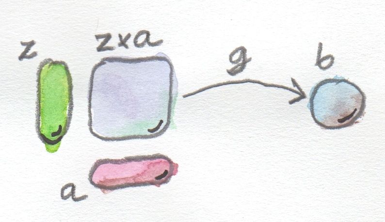
To apply the universal construction, we need to define a special property that would let us search through the category of monoids and pick the best candidate for a free monoid. But a free monoid is defined by its generators. Different choices of generators produce different free monoids (a list of Bool is not the same as a list of Int). Our construction must start with a set of generators. So we’re back to sets!

That’s where the forgetful functor comes into play. We can use it to X-ray our monoids. We can identify the generators in the X-ray images of those blobs. Here’s how it works:

We start with a set of generators, x. That’s a set in Set.

The pattern we are going to match consists of a monoid m — an object of Mon — and a function p in Set:

p :: x -> U m

where U is our forgetful functor from Mon to Set. This is a weird heterogeneous pattern — half in Mon and half in Set.

The idea is that the function p will identify the set of generators inside the X-ray image of m. It doesn’t matter that functions may be lousy at identifying points inside sets (they may collapse them). It will all be sorted out by the universal construction, which will pick the best representative of this pattern.

Monoid Pattern

We also have to define the ranking among candidates. Suppose we have another candidate: a monoid n and a function that identifies the generators in its X-ray image:

q :: x -> U n

We’ll say that m is better than n if there is a morphism of monoids (that’s a structure-preserving homomorphism):

h :: m -> n

whose image under U (remember, U is a functor, so it maps morphisms to functions) factorizes through p:

q = U h . p

If you think of p as selecting the generators in m; and q as selecting “the same” generators in n; then you can think of h as mapping these generators between the two monoids. Remember that h, by definition, preserves the monoidal structure. It means that a product of two generators in one monoid will be mapped to a product of the corresponding two generators in the second monoid, and so on.

Monoid Ranking

This ranking may be used to find the best candidate — the free monoid. Here’s the definition:

We’ll say that m (together with the function p) is the free monoid with the generators x if and only if there is a unique morphism h from m to any other monoid n (together with the function q) that satisfies the above factorization property.

Incidentally, this answers our second question. The function U h is the one that has the power to collapse multiple elements of U m to a single element of U n. This collapse corresponds to identifying some elements of the free monoid. Therefore any monoid with generators x can be obtained from the free monoid based on x by identifying some of the elements. The free monoid is the one where only the bare minimum of identifications have been made.

We’ll come back to free monoids when we talk about adjunctions.

Challenges

  1. You might think (as I did, originally) that the requirement that a homomorphism of monoids preserve the unit is redundant. After all, we know that for all a
    h a * h e = h (a * e) = h a

    So h e acts like a right unit (and, by analogy, as a left unit). The problem is that h a, for all a might only cover a subset of the target monoid. There may be a “true” unit outside of the image of h. Show that an isomorphism between monoids that preserves multiplication must automatically preserve unit.

  2. Consider a monoid homomorphism from lists of integers with concatenation to integers with multiplication. What is the image of the empty list []? Assume that all singleton lists are mapped to the integers they contain, that is [3] is mapped to 3, etc. What’s the image of [1, 2, 3, 4]? How many different lists map to the integer 12? Is there any other homomorphism between the two monoids?
  3. What is the free monoid generated by a one-element set? Can you see what it’s isomorphic to?

Next: Representable Functors.

Acknowledgments

I’d like to thank Gershom Bazerman for checking my math and logic, and André van Meulebrouck, who has been volunteering his editing help throughout this series of posts.
[twitter-follow screen_name=’BartoszMilewski’]

Lenses are a fascinating subject. Edward Kmett’s lens library is an indispensable tool in every Haskell programmer’s toolbox. I set out to write this blog post with the goal of describing some new insights into their categorical interpretation, but then I started reviewing all the different formulations of lenses and their relations to each other. So this post turned into a little summary of the theoretical underpinning of lenses.

If you’re already familiar with lenses, you may skip directly to the last section, which describes some new results.

The Data-Centric Picture

Lens

Lenses start as a very simple idea: an accessor/mutator or getter/setter pair — something familiar to every C++, Java, or C# programmer. In Haskell they can be described as two functions:

get :: s -> a
set :: s -> a -> s

Given an object of type s, the first function produces the value of the object’s sub-component of type a — which is the focus of the particular lens. The second function takes the object together with a new value for the sub-component, and produces a modified object.

A simple example is a lens that focuses on the first component of a pair:

get :: (a, a') -> a
get (x, y) = x
set :: (a, a') -> a -> (a, a')
set (x, y) x' = (x', y)

In Haskell we can go even further and define a lens for a polymorphic object, in which the setter changes not only the value of the sub-component, but also its type. This will, of course, also change the type of the resulting object. So, in general we have:

get :: s -> a
set :: s -> b -> t

Our pair example doesn’t change much on the surface:

get :: (a, a') -> a
get (x, y) = x
set :: (a, a') -> b -> (b, a')
set (x, y) x' = (x', y)

The difference is that the type of x' can now be different from the type of x. The first component of the pair is of type a before the update, and of type b (the same as that of x') after it. This way we can turn a pair of, say, (Int, Bool) to a pair of (String, Bool).

We can always go back to the monomorphic version of the lens by choosing b equal to a and t equal to s.

Not every pair of functions like these constitutes a lens. A lens has to obey a few laws (first formulated by Pierce in the database context). In particular, if you get a component after you set it, you should get back the value you just put in:

get . set s = id

If you call set with the value you obtained from get, you should get back the unchanged object:

set s (get s) = s

Finally, a set should overwrite the result of a previous set:

set (set s a) b = set s b

So this is what I would call a “classical” lens. It’s formulated in easy to understand programming terms.

The Algebraic Picture

It was Russell O’Connor who noticed that when you refactor the common element from the getter/setter pair, you get an interesting algebraic structure. Instead of writing the lens as two functions, we can write it as one function returning a pair:

s -> (a, b -> t)

Think of this as factoring out the “this” pointer in OO and returning the interface. Of course, the difference is that, in functional programming, the setter does not mutate the original — it returns a new version of the object instead.

Let’s for a moment concentrate on the monomorphic version of the lens — one in which a is the same as b, and s is the same as t. We can define a data structure:

data Store a s = Store a (a -> s)

and rewrite the lens as:

s -> Store a s

For instance, our first-component-of-a-pair lens will take the form:

fstl :: (a, b) -> Store a (a, b)
fstl (x, y) = Store x (\x' -> (x', y))

The first observation is that, for any a, Store a is a functor:

instance Functor (Store a) where
    fmap f (Store x h) = Store x (f . h)

It’s a well-known fact that you can define algebras for a functor, so-called F-algebras. An algebra for a functor f consists of a type s called the carrier type and a function called the action:

alg :: f s -> s

This is almost like a lens (with f replaced by Store a), except that the arrow goes the wrong way. Not to worry: there is a dual notion called a coalgebra. It consists of a carrier type s and a function:

coalg :: s -> f s

Substitute Store a for f and you see that a lens is nothing but a coalgebra for this functor. This is not saying much — we have just given a mathematical name to a programming construct, no big deal. Except that Store a is more than a functor — it’s also a comonad.

What’s a comonad? It’s a monad with the arrows reversed.

You know that you can define a monad in Haskell using return and join. Reverse the arrows on those two, and you get extract and duplicate, the two functions that define a comonad.

class (Functor w) => Comonad w where
    extract :: w a -> a
    duplicate :: w a -> w (w a)

Here, w is a type constructor that is also a functor.

This is how you can implement those two functions for Store a:

instance Comonad (Store a) where
    -- extract :: Store a s -> s
    extract (Store x h) = h x
    -- duplicate :: Store a s -> Store a (Store a s)
    duplicate (Store x h) = Store x (\y -> Store y h)

So now we have two structures: a comonad w and a coalgebra:

type Coalgebra w s = s -> w s

A lens is a special case of this coalgebra where w is Store a.

Every time you have two structures, you may legitimately ask the question: Are they compatible? Just by looking at types, you may figure out some obvious compatibility conditions. In particular, since they go the opposite way, it would make sense for extract to undo the action of coalg:

coalg :: Coalgebra w s
extract . coalg = id

Coalgebra Law 1

Also, duplicating the result of coalg should be the same as applying coalg twice (the second time lifted by fmap):

fmap coalg . coalg = duplicate . coalg

Coalgebra Law 2

If these two conditions are satisfied, we call coalg a comonad coalgebra.

And here’s the clencher:

These two conditions when applied to the Store a comonad are equivalent to our earlier lens laws.

Let’s see how it works. First we’ll express the result of our lens coalgebra acting on some object s in terms of get and set (curried set s is a function a->s):

coalg s = Store (get s) (set s)

The first condition extract . coalg = id immediately gives us the law:

set s (get s) = s

When we act with duplicate on coalg s, we get:

Store (get s) (\y -> Store y (set s))

On the other hand, when we fmap our coalg over coalg s, we get:

Store (get s) ((\s' -> Store (get s') (set s')) . set s)

Two functions — the second components of the Store objects in those equations — must be equal when acting on any a. The first function produces:

Store a (set s)

In the second one, we first apply set s to a to get set s a, which we then pass to the lambda to get:

Store (get (set s a)) (set (set s a))

This reproduces the other two (monomorphic) lens laws:

get (set s a) = a

and

set (set s a) = set s

This algebraic construction can be extended to type-changing lenses by replacing Store with its indexed version:

data IStore a b t = IStore a (b -> t)

and the comonad with its indexed counterpart. The indexed store is also called Context in the lens parlance, and an indexed comonad is also called a parametrized comonad.

So what’s an indexed comonad? Let’s start with an indexed functor. It’s a type constructor that takes three types, a, b, and s, and is a functor in the third argument:

class IxFunctor f where
    imap :: (s -> t) -> f a b s -> f a b t

IStore is obviously an indexed functor:

instance IxFunctor IStore where
    -- imap :: (s -> t) -> IStore a b s -> IStore a b t
    imap f (IStore x h) = IStore x (f . h)

An indexed comonad has the indexed versions of extract and duplicate:

class IxComonad w where
    iextract :: w a a t -> t
    iduplicate :: w a b t -> w a j (w j b t)

Notice that iextract is “diagonal” in the index types, whereas the double application of w shares one index, j, between the two applications. This plays very well with the unit and multiplication interpretation of a monad — here it looks just like matrix multiplication (although we are dealing with a comonad rather than a monad).

It’s easy to see that the instantiation of the indexed comonad for IStore works the same way as the instantiation of the comonad for Store. The types just work out that way.

instance IxComonad IStore where
    -- iextract :: IStore a a t -> t
    iextract (IStore a h) = h a
    -- iduplicate :: IStore a b t -> IStore a c (IStore c b t)
    iduplicate (IStore a h) = IStore a (\c -> IStore c h)

There is also an indexed version of a comonad coalgebra, where the coalgebra is replaced by a family of mappings from some carrier type s to w a b t; with the type t determined by s together with the choice of of the indexes a and b:

type ICoalg w s t a b = s -> w a b t

The compatibility conditions that make it an (indexed) comonad coalgebra are almost identical to the standard compatibility conditions, except that we have to be careful about the index types. Here’s the first condition:

icoalg_aa :: ICoalg w s t a a
iextract . icoalg_aa = id

ICoalgebra Law

Let’s analyze the types. The inner part has the type:

icoalg_aa :: s -> w a a t

We apply iextract to it, which has the type:

iextract :: w a a t -> t

and get:

iextract . icoalg_aa :: s -> t

The right hand side of the condition has the type:

id :: s -> s

It follows that, for the diagonal components of ICoalg w s t, t must be equal to s. The diagonal part of ICoalg w s t is therefore a family of regular coalgebras.

As we have done with the monomorphic lens, we can express (ICoalg IStore s t a b), when acting on s, in terms of get and set:

icoalg_ab s = IStore (get s) (set s)

But now get s is of type a, while set s if of the type b -> t. We can still apply extract to the diagonal term IStore a a t as required by the first compatibility condition. When equating the result to id, we recover the lens law:

set s (get s) = s

Similarly, it’s straightforward to see that the second compatibility condition:

icoalg_bc :: ICoalg w s t b c
icoalg_ab :: ICoalg w s t a b
icoalg_ac :: ICoalg w s t a c
imap icoalg_bc . icoalg_ab = iduplicate . icoalg_ac

is equivalent to the other two lens laws.

The Parametric Picture

Despite being theoretically attractive, standard lenses were awkward to use and, in particular, to compose. The breakthrough came when Twan van Laarhoven realized that there is a higher-order representation for them that has very nice compositional properties. Composing lenses to focus on sub-objects of sub-objects turned into simple function composition.

Here’s Twan’s representation (generalized by Russell for the polymorphic case):

type Lens s t a b = forall f. Functor f => (a -> f b) -> (s -> f t)

So a lens is a polymorphic higher order function with a twist. The twist is that it’s polymorphic with respect to a functor rather than a type.

You can think of it this way: the caller provides a function to modify a particular field of s, turning it from type a to f b. What the caller gets back is a function that transforms the whole of s to f t. The idea is that the lens knows how to reconstruct the object, while putting it under a functor f — if you tell it how to modify a field, also under this functor.

For instance, continuing with our example, here’s the van Laarhoven lens that focuses on the first component of a pair:

vL :: Lens (a, c) (b, c) a b
vL h (x, x') = fmap (\y -> (y, x')) (h x)

Here, s is (a, c) and t is (b, c).

To see that the van Laarhoven representation is equivalent to the get/set one, let’s first change the order of arguments and pull s outside of the forall quantifier:

Lens s t a b = s -> (forall f. Functor f => (a -> f b) -> f t)

Here’s how you can read this definition: For a given s, if you give me a function from a to f b, I will produce a value of type f t. And I don’t care what functor you use!

What does it mean not to care about the functor? It means that the lens must be parametrically polymorphic in f. It can’t do case analysis on a functor. It must be implemented using the same formula for f being the list functor, or the Maybe functor, or the Const functor, etc. There’s only one thing all these functors have in common, and that’s the fmap function; so that’s what we are allowed to use in the implementation of the lens.

Now let’s think what we can do with a function a -> f b that we were given. There’s only one thing: apply it to some value of type a. So we must have access to a value of type a. The result of this application is some value of type f b, but we need to produce a value of the type f t. The only way to do it is to have a function of type b->t and sneak it under the functor using fmap (so here’s where the generic functor comes in). We conclude that the implementation of the function:

forall f. Functor f => (a -> f b) -> f t

must be hiding a value of type a and a function b->t. But that’s exactly the contents of IStore a b t. Parametricity tells us that there is an IStore hiding inside the van Laarhoven lens. The lens is equivalent to:

s -> IStore a b t

In fact, with a clever choice of functors we can recover both get and set from the van Laarhoven representation.

First we select our functor to be Const a. Note that the parameter a is not the one over which the functor is defined. Const a takes a second parameter b over which it is functorial. And, even though it takes b as a type parameter, it doesn’t use it at all. Instead, like a magician, it palms an a, and then reveals it at the end of the trick.

newtype Const a b = Const { getConst :: a }

instance Functor (Const a) where
    -- fmap :: (s -> t) -> Const a s -> Const a t
    fmap _ (Const a) = (Const a)

The constructor Const happens to be a function

Const :: a -> Const a b

which has the required form to be the first argument to the lens:

a -> f b

When we apply the lens, let’s call it vL, to the function Const, we get another function:

vL Const :: s -> Const a t

We can apply this function to s, and then, in the final reveal, retrieve the value of a that was smuggled inside Const a:

get vL s = getConst $ vL Const s

Similarly, we can recover set from the van Laarhoven lens using the Identity functor:

newtype Identity a = Identity { runIdentity :: a }

We define:

set vL s x = runIdentity $ vL (Identity . const x) s

The beauty of the van Laarhoven representation is that it composes lenses using simple function composition. A lens takes a function and returns a function. This function can, in turn, be passed as the argument to another lens, and so on.

There’s an interesting twist to this kind of composition — the function composition operator in Haskell is the dot, just like the field accessor in OO languages like Java or C++; and the composition follows the same order as the composition of accessors in those languages. This was first observed by Conal Elliott in the context of semantic editor combinators.

Consider a lens that focuses on the a field inside some object s. It’s type is:

Lens s t a b

When given a function:

h :: a -> f b

it returns a function:

h' :: s -> f t

Now consider another lens that focuses on the s field inside some even bigger object u. It’s type is:

Lens u w s t

It expects a function of the type:

g :: s -> f t

We can pass the result of the first lens directly to the second lens to form a composite:

Lens u w s t . Lens s t a b

We get a lens that focuses on the a field of the object s that is the sub-object of the big object u. It works just like in Java, where you apply a dot to the result of a getter or a setter, to dig deeper into a subobject.

Not only do lenses compose using regular function composition, but we can also use the identity function as the identity lens. So lenses form a category. It’s time to have a serious look at category theory. Warning: Heavy math ahead!

The Categorical Picture

I used parametricity arguments to justify the choice of the van Laarhoven representation for the lens. The lens function is supposed to have the same form for all functors f. Parametricity arguments have an operational feel to them, which is okay, but I feel like a solid categorical justification is more valuable than any symbol-shuffling argument. So I worked on it, and eventually came up with a derivation of the van Laarhoven representation using the Yoneda lemma. Apparently Russell O’Connor and Mauro Jaskelioff had similar feelings because they came up with the same result independently. We used the same approach, going through the Store functor and applying the Yoneda lemma twice, once in the functor category, and once in the Set category (see the Bibliography).

I would like to present the same result in a more general setting of the Yoneda embedding. It’s a direct consequence of the Yoneda lemma, and it states that any category can be embedded (fully and faithfully) in the category of functors from that category to Set.

Here’s how it works: Let’s fix some object a in some category C. For any object x in that category there is a hom-set C(a, x) of morphisms from a to x. A hom-set is a set — an object in the category Set of sets. So we have defined a mapping from C to Set that takes an x and maps it to the set C(a, x). This mapping is called C(a, _), with the underscore serving as a placeholder for the argument.

Hom-Set

It’s easy to convince yourself that this mapping is in fact a functor from C to Set. Indeed, take any morphism f from x to y. We want to map this morphism to a function (a morphism in Set) that goes between C(a, x) and C(a, y). Let’s define this lifted function component-wise: given any element h from C(a, x) we can map it to f . h. It’s just a composition of two morphisms from C. The resulting morphism is a member of C(a, y). We have lifted a morphism f from C to Set thus establishing that C(a, _) is a functor.

Hom Functor

Now consider two such functors, C(a, _) and C(b, _). The Yoneda embedding theorem tells us that there is a one-to-one correspondence between the set of natural transformations between these two functors and the hom-set C(b, a).

Nat(C(a, _), C(b, _)) ≅ C(b, a)

Notice the reversed order of a and b on the right-hand side.

Yoneda Embedding

Let’s rephrase what we have just seen. For every a in C, we can define a functor C(a, _) from C to Set. Such a functor is a member of the functor category Fun(C, Set). So we have a mapping from C to the functor category Fun(C, Set). Is this mapping a functor?

We have just seen that there is a mapping between morphisms in C and natural transformations in Fun(C, Set) — that’s the gist of the Yoneda embedding. But natural transformations are morphisms in the functor category. So we do have a functor from C to the functor category Fun(C, Set). It maps objects to objects and morphisms to morphisms. It’s a contravariant functor, because of the reversal of a and b. Moreover, it maps the hom-sets in the two categories one-to-one, so it’s a fully faithful functor, and therefore it defines an embedding of categories. Every category C can be embedded in the functor category Fun(C, Set). That’s called the Yoneda embedding.

Yoneda Embedding 2

There’s an interesting consequence of the Yoneda embedding: Every functor category can be embedded in its own functor category — just replace C with a functor category in the Yoneda embedding. Recall that functors between any two categories form a category. It’s a category in which objects are functors and morphisms are natural transformations. Yoneda embedding works for that category too, which means that a functor category can be embedded in a category of functors from that functor category to Set.

Let’s see what that means. We can fix one functor, say R and consider the hom-set from R to some arbitrary functor f. Since we are in a functor category, this hom-set is a set of natural transformations between the two functors, Nat(R, f).

Now let’s pick another functor S. It also defines a set of natural transformations Nat(S, f). We can keep picking functors and mapping them to sets (sets of natural transformations). In fact we know from the previous argument that this mapping is itself a functor. This time it’s a functor from a functor category to Set.

Functor Embedding

What does the Yoneda embedding tell us about any two such functors? That the set of natural transformations between them is isomorphic to the (reversed) hom-set. But this time hom-sets are sets of natural transformations. So we have:

Nat(Nat(R, _), Nat(S, _)) ≅ Nat(S, R)

Functor Embedding 2

All natural transformations in this formula are regular natural transformation except for the outer one, which is more interesting. You may recall that a natural transformation is a family of morphisms parameterized by objects. But in this case objects are functors, and morphisms are themselves natural transformations. So it’s a family of natural transformations parameterized by functors. Keep this in mind as we proceed.

To get a better feel of what’s happening, let’s translate this to Haskell. In Haskell we represent natural transformations as polymorphic functions. This makes sense, since a natural transformation is a family of morphisms (here functions) parameterized by objects (here types). So a member of Nat(R, f) can be represented as:

forall x. R x -> f x

Similarly, the second natural transformation in our formula turns into:

forall y. S y -> f y

As I said, the outer natural transformation in the Yoneda embedding is a family of natural transformations parameterized by a functor, so we get:

forall f. Functor f => (forall x. R x -> f x) -> (forall y. S y -> f y)

You can already see one element of the van Laarhoven representation: the quantification over a functor.

The right hand side of the Yoneda embedding is a natural transformation:

forall z. S z -> R z

The next step is to pick the appropriate functors for R and S. We’ll take R to be IStore a b and S to be IStore s t.

Let’s work on the first part:

forall x. IStore a b x -> f x

A function from IStore a b x is equivalent to a function of two arguments, one of them of type a and another of type b->x:

forall x. a -> (b -> x) -> f x

We can pull a out of forall to get:

a -> (forall x. (b -> x) -> f x)

If you squint a little, you recognize that the thing in parentheses is a natural transformation between the functor C(b, _) and f, where C is the category of Haskell types. We can now apply the Yoneda lemma, which says that this set of natural transformations is isomorphic to the set f b:

forall x. (b -> x) -> f x ≅ f b

We can apply the same transformation to the second part of our identity:

forall y. (IStore s t y -> f y) ≅ s -> f t

Taking it all together, we get:

forall f. Functor f => (a -> f b) -> (s -> f t) 
    ≅ forall z. IStore s t z -> IStore a b z

Let’s now work on the right hand side:

forall z. IStore s t z -> IStore a b z 
    ≅ forall z. s -> (t -> z) -> IStore a b z

Again, pulling s out of forall and applying the Yoneda lemma, we get:

s -> IStore a b t

But that’s just the standard representation of the lens:

s -> IStore a b t ≅ (s -> a, s -> b -> t) = (get, set)

Thus the Yoneda embedding of the functor category leads to the van Laarhoven representation of the lens:

forall f. Functor f => (a -> f b) -> (s -> ft) 
  ≅ (s -> a, s -> b -> t)

Playing with Adjunctions

This is all very satisfying, but you may wonder what’s so special about the IStore functor? The crucial step in the derivation of the van Laarhoven representation was the application of the Yoneda lemma to get this identity:

forall x. IStore a b x -> f x ≅ a -> f b

Let’s rewrite it in the more categorical language:

Nat(IStore a b, f) ≅ C(a, f b)

The set of natural transformations from the functor IStore a b to the functor f is isomorphic to the hom-set between a and f b. Any time you see an isomorphism of hom-sets (and remember that Nat is the hom-set in the functor category), you should be on the lookout for an adjunction. And indeed, we have an adjunction between two functors. One functor is defined as:

a -> IStore a b

It takes an object a in C and maps it to a functor IStore a b parameterized by some other object b. The other functor is:

f -> f b

It maps a functor, an object in the functor category, to an object in C. This functor is also parameterized by the same b. Since this is a flipped application, I’ll call it Flapp:

newtype Flapp b f = Flapp (f b)

So, for any b, the functor-valued functor IStore _ b is left adjoint to Flapp b. This is what makes IStore special.

IStore Adjunction

As a side note: IStore a b is a covariant functor in a and a contravariant functor in b. However, Store a is not functorial in a, because a appears in both positive and negative position in its definition. So the adjunction trick doesn’t work for a simple (monomorphic) lens.

We can now turn the tables and use the adjunction to define the functor IStore in an arbitrary category (notice that the Yoneda lemma worked only for Set-valued functors). We just define a functor-valued functor IStore to be the left adjoint to Flapp, provided it exists.

Nat(IStore a b, f) ≅ C(a, f b)

Here, Nat is a set of natural transformations between endofunctors in C.

We can substitute the so defined functor into the Yoneda embedding formula we used earlier:

Nat((Nat(IStore a b, f), Nat(IStore s t, f)) 
    ≅ Nat(IStore s t, IStore a b)

We can now use the adjunction, rather than the Yoneda lemma, to eliminate some of the occurrences IStore:

Nat(C(a, f b), C(s, f t))
    ≅ C(s, IStore a b t)

This is slightly more general than the original van Laarhoven equivalence.

We can go even farther and reproduce the Jaskelioff and O’Connor trick of constraining the generic functor in the definition of the van Laarhoven lens to a pointed or applicative functor. This results in a multi-focus lens. In particular, if we use pointed functors, we get lenses with zero or one targets, so called affine lenses. Restricting the functors further to applicative leads to lenses with any number of targets, or traversals.

The trick is that any pointed or applicative functor can be stripped of the additional functionality and treated just like any other functor. This act of “forgetting” about pure and <*> may itself be considered a functor in the functor category. It’s called, appropriately, a forgetful functor. The left adjoint to a forgetful functor (if it exists) is called a free functor. It takes an arbitrary functor and creates a pointed functor by generating an artificial pure; or it creates an applicative functor by adding <*>. This adjunction is described by a natural isomorphism of hom-sets — in this case sets of natural transformations:

Nat(S, U f) ≅ Nat(S*, f)

Here, U is the forgetful functor, and S* is the free applicative/pointed version of the functor S. The functor f ranges across applicative (respectively, pointed) functors.

Now we can try to substitute the free version of IStore in the Yoneda embedding formula:

Nat((Nat(IStore* a b, f), Nat(IStore* s t, f)) 
    ≅ Nat(IStore* s t, IStore* a b)

The formula holds for any applicative (pointed) functor f and a set of natural transformations over such functors.

The first step is to use the forgetful/free adjunction:

Nat((Nat(IStore a b, U f), Nat(IStore s t, U f)) 
    ≅ Nat(IStore s t, U IStore* a b)

Then we can use our defining adjunction for IStore to get:

Nat(C(a, U f b), C(s, U f t)) 
    ≅ C(s, U IStore* a b t)

In Haskell notation this reads:

forall f. Applicative f => (a -> f b) -> (s -> f t)
    ≅ s -> IAppStore a b t

(the action of U is implicit).

The free applicative version of IStore is defined as:

data IAppStore a b t = 
    Unit t
  | IAppStore a (IAppStore a b (b -> t))

These are all known results, but the use of the Yoneda embedding and the adjunction to define the IStore functor makes the derivation more compact and slightly more general.

Acknowledgments

I’m grateful to Mauro Jaskelioff, Gershom Bazerman, and Joseph Abrahamson for reading the draft and providing helpful comments and to André van Meulebrouck for editing help.

Bibliography

  1. Edward Kmett, The Haskell Lens Library
  2. Simon Peyton Jones, Lenses: Compositional Data Access and Manipulation. A Skills Matter video presentation.
  3. Joseph Abrahamson, A Little Lens Starter Tutorial
  4. Joseph Abrahamson, Lenses from Scratch
  5. Artyom, lens over tea tutorial
  6. Twan van Laarhoven, CPS based functional references
  7. Bartosz Milewski, Lenses, Stores, and Yoneda
  8. Mauro Jaskelioff, Russell O’Connor, A Representation Theorem for Second-Order Functionals
  9. Bartosz Milewski, Understanding Yoneda

I am sometimes asked by C++ programmers to give an example of a problem that can’t be solved without monads. This is the wrong kind of question — it’s like asking if there is a problem that can’t be solved without for loops. Obviously, if your language supports a goto, you can live without for loops. What monads (and for loops) can do for you is to help you structure your code. The use of loops and if statements lets you convert spaghetti code into structured code. Similarly, the use of monads lets you convert imperative code into declarative code. These are the kind of transformations that make code easier to write, understand, maintain, and generalize.

So here’s a problem that you may get as an interview question. It’s a small problem, so the advantages of various approaches might not be immediately obvious, especially if you’ve been trained all your life in imperative programming, and you are seeing monads for the first time.

You’re supposed write a program to solve this puzzle:

  s e n d
+ m o r e
---------
m o n e y

Each letter correspond to a different digit between 0 and 9. Before you continue reading this post, try to think about how you would approach this problem.

The Analysis

It never hurts to impress your interviewer with your general knowledge by correctly classifying the problem. This one belongs to the class of “constraint satisfaction problems.” The obvious constraint is that the numbers obtained by substituting letters with digits have to add up correctly. There are also some less obvious constraints, namely the numbers should not start with zero.

If you were to solve this problem using pencil and paper, you would probably come up with lots of heuristics. For instance, you would deduce that m must stand for 1 because that’s the largest possible carry from the addition of two digits (even if there is a carry from the previous column). Then you’d figure out that s must be either 8 or 9 to produce this carry, and so on. Given enough time, you could probably write an expert system with a large set of rules that could solve this and similar problems. (Mentioning an expert system could earn you extra points with the interviewer.)

However, the small size of the problem suggests that a simple brute force approach is probably best. The interviewer might ask you to estimate the number of possible substitutions, which is 10!/(10 – 8)! or roughly 2 million. That’s not a lot. So, really, the solution boils down to generating all those substitutions and testing the constraints for each.

The Straightforward Solution

The mind of an imperative programmer immediately sees the solution as a set of 8 nested loops (there are 8 unique letters in the problem: s, e, n, d, m, o, r, y). Something like this:

for (int s = 0; s < 10; ++s)
    for (int e = 0; e < 10; ++e)
        for (int n = 0; n < 10; ++n)
            for (int d = 0; d < 10; ++d)
                ...

and so on, until y. But then there is the condition that the digits have to be different, so you have to insert a bunch of tests like:

e != s
n != s && n != e
d != s && d != e && d != n

and so on, the last one involving 7 inequalities… Effectively you have replaced the uniqueness condition with 28 new constraints.

This would probably get you through the interview at Microsoft, Google, or Facebook, but really, can’t you do better than that?

The Smart Solution

Before I proceed, I should mention that what follows is almost a direct translation of a Haskell program from the blog post by Justin Le. I strongly encourage everybody to learn some Haskell, but in the meanwhile I’ll be happy to serve as your translator.

The problem with our naive solution is the 28 additional constraints. Well, I guess one could live with that — except that this is just a tiny example of a whole range of constraint satisfaction problems, and it makes sense to figure out a more general approach.

The problem can actually be formulated as a superposition of two separate concerns. One deals with the depth and the other with the breadth of the search for solutions.

Let me touch on the depth issue first. Let’s consider the problem of creating just one substitution of letters with numbers. This could be described as picking 8 digits from a list of 0, 1, …9, one at a time. Once a digit is picked, it’s no longer in the list. We don’t want to hard code the list, so we’ll make it a parameter to our algorithm. Notice that this approach works even if the list contains duplicates, or if the list elements are not easily comparable for equality (for instance, if they are futures). We’ll discuss the list-picking part of the problem in more detail later.

Now let’s talk about breadth: we have to repeat the above process for all possible picks. This is what the 8 nested loops were doing. Except that now we are in trouble because each individual pick is destructive. It removes items from the list — it mutates the list. This is a well known problem when searching through solution spaces, and the standard remedy is called backtracking. Once you have processed a particular candidate, you put the elements back in the list, and try the next one. Which means that you have to keep track of your state, either implicitly on your function’s stack, or in a separate explicit data structure.

Wait a moment! Weren’t we supposed to talk about functional programming? So what’s all this talk about mutation and state? Well, who said you can’t have state in functional programming? Functional programmers have been using the state monad since time immemorial. And mutation is not an issue if you’re using persistent data structures. So fasten your seat belts and make sure your folding trays are in the upright position.

The List Monad

We’ll start with a small refresher in quantum mechanics. As you may remember from school, quantum processes are non-deterministic. You may repeat the same experiment many times and every time get a different result. There is a very interesting view of quantum mechanics called the many-worlds interpretation, in which every experiment gives rise to multiple alternate histories. So if the spin of an electron may be measured as either up or down, there will be one universe in which it’s up, and one in which it’s down.

Selections

We’ll use the same approach to solving our puzzle. We’ll create an alternate universe for each digit substitution for a given letter. So we’ll start with 10 universes for the letter s; then we’ll split each of them into ten universes for the letter e, and so on. Of course, most of these universes won’t yield the desired result, so we’ll have to destroy them. I know, it seems kind of wasteful, but in functional programming it’s easy come, easy go. The creation of a new universe is relatively cheap. That’s because new universes are not that different from their parent universes, and they can share almost all of their data. That’s the idea behind persistent data structures. These are the immutable data structures that are “mutated” by cloning. A cloned data structure shares most of its implementation with the parent, except for a small delta. We’ll be using persistent lists described in my earlier post.

Once you internalize the many-worlds approach to programming, the implementation is pretty straightforward. First, we need functions that generate new worlds. Since we are cheap, we’ll only generate the parts that are different. So what’s the difference between all the worlds that we get when selecting the substitution for the letter s? Just the number that we assign to s. There are ten worlds corresponding to the ten possible digits (we’ll deal with the constraints like s being different from zero later). So all we need is a function that generates a list of ten digits. These are our ten universes in a nutshell. They share everything else.

Once you are in an alternate universe, you have to continue with your life. In functional programming, the rest of your life is just a function called a continuation. I know it sounds like a horrible simplification. All your actions, emotions, and hopes reduced to just one function. Well, maybe the continuation just describes one aspect of your life, the computational part, and you can still hold on to our emotions.

So what do our lives look like, and what do they produce? The input is the universe we’re in, in particular the one number that was picked for us. But since we live in a quantum universe, the outcome is a multitude of universes. So a continuation takes a number, and produces a list. It doesn’t have to be a list of numbers, just a list of whatever characterizes the differences between alternate universes. In particular, it could be a list of different solutions to our puzzle — triples of numbers corresponding to “send”, “more”, and “money”. (There is actually only one solution, but that’s beside the point.)

And what’s the very essence of this new approach? It’s the binding of the selection of the universes to the continuation. That’s where the action is. This binding, again, can be expressed as a function. It’s a function that takes a list of universes and a continuation that produces a list of universes. It returns an even bigger list of universes. We’ll call this function for_each, and we’ll make it as generic as possible. We won’t assume anything about the type of the universes that are passed in, or the type of the universes that the continuation k produces. We’ll also make the type of the continuation a template parameter and extract the return type from it using auto and decltype:

template<class A, class F>
auto for_each(List<A> lst, F k) -> decltype(k(lst.front()))
{
    using B = decltype(k(lst.front()).front());
    // This should really be expressed using concepts
    static_assert(std::is_convertible<
        F, std::function<List<B>(A)>>::value,
        "for_each requires a function type List<B>(A)");

    List<List<B>> lstLst = fmap(k, lst);
    return concatAll(lstLst);
}

The function fmap is similar to std::transform. It applies the continuation k to every element of the list lst. Because k itself produces a list, the result is a list of lists, lstLst. The function concatAll concatenates all those lists into one big list.

Congratulations! You have just seen a monad. This one is called the list monad and it’s used to model non-deterministic processes. The monad is actually defined by two functions. One of them is for_each, and here’s the other one:

template<class A>
List<A> yield(A a)
{
    return List<A> (a);
}

It’s a function that returns a singleton list. We use yield when we are done multiplying universes and we just want to return a single value. We use it to create a single-valued continuation. It represents the lonesome boring life, devoid of any choices.

I will later rename these functions to mbind and mreturn, because they are part of any monad, not just the list monad.

The names like for_each or yield have a very imperative ring to them. That’s because, in functional programming, monadic code plays a role similar to imperative code. But neither for_each nor yield are control structures — they are functions. In particular for_each, which sounds and works like a loop, is just a higher order function; and so is fmap, which is used in its implementation. Of course, at some level the code becomes imperative — fmap can either be implemented recursively or using an actual loop — but the top levels are just declarations of functions. Hence, declarative programming.

There is a slight difference between a loop and a function on lists like for_each: for_each takes a whole list as an argument, while a loop might generate individual items — in this case integers — on the fly. This is not a problem in a lazy functional language like Haskell, where a list is evaluated on demand. The same behavior may be implemented in C++ using streams or lazy ranges. I won’t use it here, since the lists we are dealing with are short, but you can read more about it in my earlier post Getting Lazy with C++.

We are not ready yet to implement the solution to our puzzle, but I’d like to give you a glimpse of what it looks like. For now, think of StateL as just a list. See if it starts making sense (I grayed out the usual C++ noise):

StateL<tuple<int, int, int>> solve()
{
    StateL<int> sel = &select<int>;

    return for_each(sel, [=](int s) {
    return for_each(sel, [=](int e) {
    return for_each(sel, [=](int n) {
    return for_each(sel, [=](int d) {
    return for_each(sel, [=](int m) {
    return for_each(sel, [=](int o) {
    return for_each(sel, [=](int r) {
    return for_each(sel, [=](int y) {
        return yield_if(s != 0 && m != 0, [=]() {
            int send  = asNumber(vector{s, e, n, d});
            int more  = asNumber(vector{m, o, r, e});
            int money = asNumber(vector{m, o, n, e, y});
            return yield_if(send + more == money, [=]() {
                return yield(make_tuple(send, more, money));
            });
        });
    });});});});});});});});
}

The first for_each takes a selection of integers, sel, (never mind how we deal with uniqueness); and a continuation, a lambda, that takes one integer, s, and produces a list of solutions — tuples of three integers. This continuation, in turn, calls for_each with a selection for the next letter, e, and another continuation that returns a list of solutions, and so on.

The innermost continuation is a conditional version of yield called yield_if. It checks a condition and produces a zero- or one-element list of solutions. Internally, it calls another yield_if, which calls the ultimate yield. If that final yield is called (and it might not be, if one of the previous conditions fails), it will produce a solution — a triple of numbers. If there is more than one solution, these singleton lists will get concatenated inside for_each while percolating to the top.

In the second part of this post I will come back to the problem of picking unique numbers and introduce the state monad. You can also have a peek at the code on github.

Challenges

  1. Implement for_each and yield for a vector instead of a List. Use the Standard Library transform instead of fmap.
  2. Using the list monad (or your vector monad), write a function that generates all positions on a chessboard as pairs of characters between 'a' and 'h' and numbers between 1 and 8.
  3. Implement a version of for_each (call it repeat) that takes a continuation k of the type function<List<B>()> (notice the void argument). The function repeat calls k for each element of the list lst, but it ignores the element itself.

This is part 10 of Categories for Programmers. Previously: Function Types. See the Table of Contents.

We talked about functors as mappings between categories that preserve their structure. A functor “embeds” one category in another. It may collapse multiple things into one, but it never breaks connections. One way of thinking about it is that with a functor we are modeling one category inside another. The source category serves as a model, a blueprint, for some structure that’s part of the target category.

1_Functors

There may be many ways of embedding one category in another. Sometimes they are equivalent, sometimes very different. One may collapse the whole source category into one object, another may map every object to a different object and every morphism to a different morphism. The same blueprint may be realized in many different ways. Natural transformations help us compare these realizations. They are mappings of functors — special mappings that preserve their functorial nature.

Consider two functors F and G between categories C and D. If you focus on just one object a in C, it is mapped to two objects: F a and G a. A mapping of functors should therefore map F a to G a.

2_NatComp

Notice that F a and G a are objects in the same category D. Mappings between objects in the same category should not go against the grain of the category. We don’t want to make artificial connections between objects. So it’s natural to use existing connections, namely morphisms. A natural transformation is a selection of morphisms: for every object a, it picks one morphism from F a to G a. If we call the natural transformation α, this morphism is called the component of α at a, or αa.

αa :: F a -> G a

Keep in mind that a is an object in C while αa is a morphism in D.

If, for some a, there is no morphism between F a and G a in D, there can be no natural transformation between F and G.

Of course that’s only half of the story, because functors not only map objects, they map morphisms as well. So what does a natural transformation do with those mappings? It turns out that the mapping of morphisms is fixed — under any natural transformation between F and G, F f must be transformed into G f. What’s more, the mapping of morphisms by the two functors drastically restricts the choices we have in defining a natural transformation that’s compatible with it. Consider a morphism f between two objects a and b in C. It’s mapped to two morphisms, F f and G f in D:

F f :: F a -> F b
G f :: G a -> G b

The natural transformation α provides two additional morphisms that complete the diagram in D:

αa :: F a -> G a
αb :: F b -> G b

3_Naturality

Now we have two ways of getting from F a to G b. To make sure that they are equal, we must impose the naturality condition that holds for any f:

G f ∘ αa = αb ∘ F f

The naturality condition is a pretty stringent requirement. For instance, if the morphism F f is invertible, naturality determines αb in terms of αa. It transports αa along f:

αb = (G f) ∘ αa ∘ (F f)-1

4_Transport

If there is more than one invertible morphism between two objects, all these transports have to agree. In general, though, morphisms are not invertible; but you can see that the existence of natural transformations between two functors is far from guaranteed. So the scarcity or the abundance of functors that are related by natural transformations may tell you a lot about the structure of categories between which they operate. We’ll see some examples of that when we talk about limits and the Yoneda lemma.

Looking at a natural transformation component-wise, one may say that it maps objects to morphisms. Because of the naturality condition, one may also say that it maps morphisms to commuting squares — there is one commuting naturality square in D for every morphism in C.

Naturality

This property of natural transformations comes in very handy in a lot of categorical constructions, which often include commuting diagrams. With a judicious choice of functors, a lot of these commutativity conditions may be transformed into naturality conditions. We’ll see examples of that when we get to limits, colimits, and adjunctions.

Finally, natural transformations may be used to define isomorphisms of functors. Saying that two functors are naturally isomorphic is almost like saying they are the same. Natural isomorphism is defined as a natural transformation whose components are all isomorphisms (invertible morphisms).

Polymorphic Functions

We talked about the role of functors (or, more specifically, endofunctors) in programming. They correspond to type constructors that map types to types. They also map functions to functions, and this mapping is implemented by a higher order function fmap (or transform, then, and the like in C++).

To construct a natural transformation we start with an object, here a type, a. One functor, F, maps it to the type F a. Another functor, G, maps it to G a. The component of a natural transformation alpha at a is a function from F a to G a. In pseudo-Haskell:

alphaa :: F a -> G a

A natural transformation is a polymorphic function that is defined for all types a:

alpha :: forall a . F a -> G a

The forall a is optional in Haskell (and in fact requires turning on the language extension ExplicitForAll). Normally, you would write it like this:

alpha :: F a -> G a

Keep in mind that it’s really a family of functions parameterized by a. This is another example of the terseness of the Haskell syntax. A similar construct in C++ would be slightly more verbose:

template<class A> G<A> alpha(F<A>);

There is a more profound difference between Haskell’s polymorphic functions and C++ generic functions, and it’s reflected in the way these functions are implemented and type-checked. In Haskell, a polymorphic function must be defined uniformly for all types. One formula must work across all types. This is called parametric polymorphism.

C++, on the other hand, supports by default ad hoc polymorphism, which means that a template doesn’t have to be well-defined for all types. Whether a template will work for a given type is decided at instantiation time, where a concrete type is substituted for the type parameter. Type checking is deferred, which unfortunately often leads to incomprehensible error messages.

In C++, there is also a mechanism for function overloading and template specialization, which allows different definitions of the same function for different types. In Haskell this functionality is provided by type classes and type families.

Haskell’s parametric polymorphism has an unexpected consequence: any polymorphic function of the type:

alpha :: F a -> G a

where F and G are functors, automatically satisfies the naturality condition. Here it is in categorical notation (f is a function f::a->b):

G f ∘ αa = αb ∘ F f

In Haskell, the action of a functor G on a morphism f is implemented using fmap. I’ll first write it in pseudo-Haskell, with explicit type annotations:

fmapG f . alphaa = alphab . fmapF f

Because of type inference, these annotations are not necessary, and the following equation holds:

fmap f . alpha = alpha . fmap f

This is still not real Haskell — function equality is not expressible in code — but it’s an identity that can be used by the programmer in equational reasoning; or by the compiler, to implement optimizations.

The reason why the naturality condition is automatic in Haskell has to do with “theorems for free.” Parametric polymorphism, which is used to define natural transformations in Haskell, imposes very strong limitations on the implementation — one formula for all types. These limitations translate into equational theorems about such functions. In the case of functions that transform functors, free theorems are the naturality conditions. [You may read more about free theorems in my blog Parametricity: Money for Nothing and Theorems for Free.]

One way of thinking about functors in Haskell that I mentioned earlier is to consider them generalized containers. We can continue this analogy and consider natural transformations to be recipes for repackaging the contents of one container into another container. We are not touching the items themselves: we don’t modify them, and we don’t create new ones. We are just copying (some of) them, sometimes multiple times, into a new container.

The naturality condition becomes the statement that it doesn’t matter whether we modify the items first, through the application of fmap, and repackage later; or repackage first, and then modify the items in the new container, with its own implementation of fmap. These two actions, repackaging and fmapping, are orthogonal. “One moves the eggs, the other boils them.”

Let’s see a few examples of natural transformations in Haskell. The first is between the list functor, and the Maybe functor. It returns the head of the list, but only if the list is non-empty:

safeHead :: [a] -> Maybe a
safeHead [] = Nothing
safeHead (x:xs) = Just x

It’s a function polymorphic in a. It works for any type a, with no limitations, so it is an example of parametric polymorphism. Therefore it is a natural transformation between the two functors. But just to convince ourselves, let’s verify the naturality condition.

fmap f . safeHead = safeHead . fmap f

We have two cases to consider; an empty list:

fmap f (safeHead []) = fmap f Nothing = Nothing
safeHead (fmap f []) = safeHead [] = Nothing

and a non-empty list:

fmap f (safeHead (x:xs)) = fmap f (Just x) = Just (f x)
safeHead (fmap f (x:xs)) = safeHead (f x : fmap f xs) = Just (f x)

I used the implementation of fmap for lists:

fmap f [] = []
fmap f (x:xs) = f x : fmap f xs

and for Maybe:

fmap f Nothing = Nothing
fmap f (Just x) = Just (f x)

An interesting case is when one of the functors is the trivial Const functor. A natural transformation from or to a Const functor looks just like a function that’s either polymorphic in its return type or in its argument type.

For instance, length can be thought of as a natural transformation from the list functor to the Const Int functor:

length :: [a] -> Const Int a
length [] = Const 0
length (x:xs) = Const (1 + unConst (length xs))

Here, unConst is used to peel off the Const constructor:

unConst :: Const c a -> c
unConst (Const x) = x

Of course, in practice length is defined as:

length :: [a] -> Int

which effectively hides the fact that it’s a natural transformation.

Finding a parametrically polymorphic function from a Const functor is a little harder, since it would require the creation of a value from nothing. The best we can do is:

scam :: Const Int a -> Maybe a
scam (Const x) = Nothing

Another common functor that we’ve seen already, and which will play an important role in the Yoneda lemma, is the Reader functor. I will rewrite its definition as a newtype:

newtype Reader e a = Reader (e -> a)

It is parameterized by two types, but is (covariantly) functorial only in the second one:

instance Functor (Reader e) where  
    fmap f (Reader g) = Reader (\x -> f (g x))

For every type e, you can define a family of natural transformations from Reader e to any other functor f. We’ll see later that the members of this family are always in one to one correspondence with the elements of f e (the Yoneda lemma).

For instance, consider the somewhat trivial unit type () with one element (). The functor Reader () takes any type a and maps it into a function type ()->a. These are just all the functions that pick a single element from the set a. There are as many of these as there are elements in a. Now let’s consider natural transformations from this functor to the Maybe functor:

alpha :: Reader () a -> Maybe a

There are only two of these, dumb and obvious:

dumb (Reader _) = Nothing

and

obvious (Reader g) = Just (g ())

(The only thing you can do with g is to apply it to the unit value ().)

And, indeed, as predicted by the Yoneda lemma, these correspond to the two elements of the Maybe () type, which are Nothing and Just (). We’ll come back to the Yoneda lemma later — this was just a little teaser.

Beyond Naturality

A parametrically polymorphic function between two functors (including the edge case of the Const functor) is always a natural transformation. Since all standard algebraic data types are functors, any polymorphic function between such types is a natural transformation.

We also have function types at our disposal, and those are functorial in their return type. We can use them to build functors (like the Reader functor) and define natural transformations that are higher-order functions.

However, function types are not covariant in the argument type. They are contravariant. Of course contravariant functors are equivalent to covariant functors from the opposite category. Polymorphic functions between two contravariant functors are still natural transformations in the categorical sense, except that they work on functors from the opposite category to Haskell types.

You might remember the example of a contravariant functor we’ve looked at before:

newtype Op r a = Op (a -> r)

This functor is contravariant in a:

instance Contravariant (Op r) where
    contramap f (Op g) = Op (g . f)

We can write a polymorphic function from, say, Op Bool to Op String:

predToStr (Op f) = Op (\x -> if f x then "T" else "F")

But since the two functors are not covariant, this is not a natural transformation in Hask. However, because they are both contravariant, they satisfy the “opposite” naturality condition:

contramap f . predToStr = predToStr . contramap f

Notice that the function f must go in the opposite direction than what you’d use with fmap, because of the signature of contramap:

contramap :: (b -> a) -> (Op Bool a -> Op Bool b)

Are there any type constructors that are not functors, whether covariant or contravariant? Here’s one example:

a -> a

This is not a functor because the same type a is used both in the negative (contravariant) and positive (covariant) position. You can’t implement fmap or contramap for this type. Therefore a function of the signature:

(a -> a) -> f a

where f is an arbitrary functor, cannot be a natural transformation. Interestingly, there is a generalization of natural transformations, called dinatural transformations, that deals with such cases. We’ll get to them when we discuss ends.

Functor Category

Now that we have mappings between functors — natural transformations — it’s only natural to ask the question whether functors form a category. And indeed they do! There is one category of functors for each pair of categories, C and D. Objects in this category are functors from C to D, and morphisms are natural transformations between those functors.

We have to define composition of two natural transformations, but that’s quite easy. The components of natural transformations are morphisms, and we know how to compose morphisms.

Indeed, let’s take a natural transformation α from functor F to G. Its component at object a is some morphism:

αa :: F a -> G a

We’d like to compose α with β, which is a natural transformation from functor G to H. The component of β at a is a morphism:

βa :: G a -> H a

These morphisms are composable and their composition is another morphism:

βa ∘ αa :: F a -> H a

We will use this morphism as the component of the natural transformation β ⋅ α — the composition of two natural transformations β after α:

(β ⋅ α)a = βa ∘ αa

5_Vertical

One (long) look at a diagram convinces us that the result of this composition is indeed a natural transformation from F to H:

H f ∘ (β ⋅ α)a = (β ⋅ α)b ∘ F f

6_VerticalNaturality

Composition of natural transformations is associative, because their components, which are regular morphisms, are associative with respect to their composition.

Finally, for each functor F there is an identity natural transformation 1F whose components are the identity morphisms:

idF a :: F a -> F a

So, indeed, functors form a category.

A word about notation. Following Saunders Mac Lane I use the dot for the kind of natural transformation composition I have just described. The problem is that there are two ways of composing natural transformations. This one is called the vertical composition, because the functors are usually stacked up vertically in the diagrams that describe it. Vertical composition is important in defining the functor category. I’ll explain horizontal composition shortly.

6a_Vertical

The functor category between categories C and D is written as Fun(C, D), or [C, D], or sometimes as DC. This last notation suggests that a functor category itself might be considered a function object (an exponential) in some other category. Is this indeed the case?

Let’s have a look at the hierarchy of abstractions that we’ve been building so far. We started with a category, which is a collection of objects and morphisms. Categories themselves (or, strictly speaking small categories, whose objects form sets) are themselves objects in a higher-level category Cat. Morphisms in that category are functors. A Hom-set in Cat is a set of functors. For instance Cat(C, D) is a set of functors between two categories C and D.

7_CatHomSet

A functor category [C, D] is also a set of functors between two categories (plus natural transformations as morphisms). Its objects are the same as the members of Cat(C, D). Moreover, a functor category, being a category, must itself be an object of Cat (it so happens that the functor category between two small categories is itself small). We have a relationship between a Hom-set in a category and an object in the same category. The situation is exactly like the exponential object that we’ve seen in the last section. Let’s see how we can construct the latter in Cat.

As you may remember, in order to construct an exponential, we need to first define a product. In Cat, this turns out to be relatively easy, because small categories are sets of objects, and we know how to define cartesian products of sets. So an object in a product category C × D is just a pair of objects, (c, d), one from C and one from D. Similarly, a morphism between two such pairs, (c, d) and (c', d'), is a pair of morphisms, (f, g), where f :: c -> c' and g :: d -> d'. These pairs of morphisms compose component-wise, and there is always an identity pair that is just a pair of identity morphisms. To make the long story short, Cat is a full-blown cartesian closed category in which there is an exponential object DC for any pair of categories. And by “object” in Cat I mean a category, so DC is a category, which we can identify with the functor category between C and D.

2-Categories

With that out of the way, let’s have a closer look at Cat. By definition, any Hom-set in Cat is a set of functors. But, as we have seen, functors between two objects have a richer structure than just a set. They form a category, with natural transformations acting as morphisms. Since functors are considered morphisms in Cat, natural transformations are morphisms between morphisms.

This richer structure is an example of a 2-category, a generalization of a category where, besides objects and morphisms (which might be called 1-morphisms in this context), there are also 2-morphisms, which are morphisms between morphisms.

In the case of Cat seen as a 2-category we have:

  • Objects: (Small) categories
  • 1-morphisms: Functors between categories
  • 2-morphisms: Natural transformations between functors.

Instead of a Hom-set between two categories C and D, we have a Hom-category — the functor category DC. We have regular functor composition: a functor F from DC composes with a functor G from ED to give G ∘ F from EC. But we also have composition inside each Hom-category — vertical composition of natural transformations, or 2-morphisms, between functors.

8_Cat-2-Cat

With two kinds of composition in a 2-category, the question arises: How do they interact with each other?

Let’s pick two functors, or 1-morphisms, in Cat:

F :: C -> D
G :: D -> E

and their composition:

G ∘ F :: C -> E

Suppose we have two natural transformations, α and β, that act, respectively, on functors F and G:

α :: F -> F'
β :: G -> G'

10_Horizontal

Notice that we cannot apply vertical composition to this pair, because the target of α is different from the source of β. In fact they are members of two different functor categories: D C and E D. We can, however, apply composition to the functors F’ and G’, because the target of F’ is the source of G’ — it’s the category D. What’s the relation between the functors G’∘ F’ and G ∘ F?

Having α and β at our disposal, can we define a natural transformation from G ∘ F to G’∘ F’? Let me sketch the construction.

9_Horizontal

As usual, we start with an object a in C. Its image splits into two objects in D: F a and F'a. There is also a morphism, a component of α, connecting these two objects:

αa :: F a -> F'a

When going from D to E, these two objects split further into four objects:

G (F a), G'(F a), G (F'a), G'(F'a)

We also have four morphisms forming a square. Two of these morphisms are the components of the natural transformation β:

βF a :: G (F a) -> G'(F a)
βF'a :: G (F'a) -> G'(F'a)

The other two are the images of αa under the two functors (functors map morphisms):

G αa :: G (F a) -> G (F'a)
G'αa :: G'(F a) -> G'(F'a)

That’s a lot of morphisms. Our goal is to find a morphism that goes from G (F a) to G'(F'a), a candidate for the component of a natural transformation connecting the two functors G ∘ F and G’∘ F’. In fact there’s not one but two paths we can take from G (F a) to G'(F'a):

G'αa ∘ βF a
βF'a ∘ G αa

Luckily for us, they are equal, because the square we have formed turns out to be the naturality square for β.

We have just defined a component of a natural transformation from G ∘ F to G’∘ F’. The proof of naturality for this transformation is pretty straightforward, provided you have enough patience.

We call this natural transformation the horizontal composition of α and β:

β ∘ α :: G ∘ F -> G'∘ F'

Again, following Mac Lane I use the small circle for horizontal composition, although you may also encounter star in its place.

Here’s a categorical rule of thumb: Every time you have composition, you should look for a category. We have vertical composition of natural transformations, and it’s part of the functor category. But what about the horizontal composition? What category does that live in?

The way to figure this out is to look at Cat sideways. Look at natural transformations not as arrows between functors but as arrows between categories. A natural transformation sits between two categories, the ones that are connected by the functors it transforms. We can think of it as connecting these two categories.

Sideways

Let’s focus on two objects of Cat — categories C and D. There is a set of natural transformations that go between functors that connect C to D. These natural transformations are our new arrows from C to D. By the same token, there are natural transformations going between functors that connect D to E, which we can treat as new arrows going from D to E. Horizontal composition is the composition of these arrows.

We also have an identity arrow going from C to C. It’s the identity natural transformation that maps the identity functor on C to itself. Notice that the identity for horizontal composition is also the identity for vertical composition, but not vice versa.

Finally, the two compositions satisfy the interchange law:

(β' ⋅ α') ∘ (β ⋅ α) = (β' ∘ β) ⋅ (α' ∘ α)

I will quote Saunders Mac Lane here: The reader may enjoy writing down the evident diagrams needed to prove this fact.

There is one more piece of notation that might come in handy in the future. In this new sideways interpretation of Cat there are two ways of getting from object to object: using a functor or using a natural transformation. We can, however, re-interpret the functor arrow as a special kind of natural transformation: the identity natural transformation acting on this functor. So you’ll often see this notation:

F ∘ α

where F is a functor from D to E, and α is a natural transformation between two functors going from C to D. Since you can’t compose a functor with a natural transformation, this is interpreted as a horizontal composition of the identity natural transformation 1F after α.

Similarly:

α ∘ F

is a horizontal composition of α after 1F.

Conclusion

This concludes the first part of the book. We’ve learned the basic vocabulary of category theory. You may think of objects and categories as nouns; and morphisms, functors, and natural transformations as verbs. Morphisms connect objects, functors connect categories, natural transformations connect functors.

But we’ve also seen that, what appears as an action at one level of abstraction, becomes an object at the next level. A set of morphisms turns into a function object. As an object, it can be a source or a target of another morphism. That’s the idea behind higher order functions.

A functor maps objects to objects, so we can use it as a type constructor, or a parametric type. A functor also maps morphisms, so it is a higher order function — fmap. There are some simple functors, like Const, product, and coproduct, that can be used to generate a large variety of algebraic data types. Function types are also functorial, both covariant and contravariant, and can be used to extend algebraic data types.

Functors may be looked upon as objects in the functor category. As such, they become sources and targets of morphisms: natural transformations. A natural transformation is a special type of polymorphic function.

Challenges

  1. Define a natural transformation from the Maybe functor to the list functor. Prove the naturality condition for it.
  2. Define at least two different natural transformations between Reader () and the list functor. How many different lists of () are there?
  3. Continue the previous exercise with Reader Bool and Maybe.
  4. Show that horizontal composition of natural transformation satisfies the naturality condition (hint: use components). It’s a good exercise in diagram chasing.
  5. Write a short essay about how you may enjoy writing down the evident diagrams needed to prove the interchange law.
  6. Create a few test cases for the opposite naturality condition of transformations between different Op functors. Here’s one choice:
    op :: Op Bool Int
    op = Op (\x -> x > 0)

    and

    f :: String -> Int
    f x = read x

Next: Declarative Programming.

Acknowledgments

I’d like to thank Gershom Bazerman for checking my math and logic, and André van Meulebrouck, who has been volunteering his editing help.
[twitter-follow screen_name=’BartoszMilewski’]

This is part 9 of Categories for Programmers. Previously: Functoriality. See the Table of Contents.

So far I’ve been glossing over the meaning of function types. A function type is different from other types.

Take Integer, for instance: It’s just a set of integers. Bool is a two element set. But a function type a->b is more than that: it’s a set of morphisms between objects a and b. A set of morphisms between two objects in any category is called a hom-set. It just so happens that in the category Set every hom-set is itself an object in the same category —because it is, after all, a set.

Hom-set in Set is just a set

Hom-set in Set is just a set

The same is not true of other categories where hom-sets are external to a category. They are even called external hom-sets.

Hom-set in category C is an external set

Hom-set in category C is an external set

It’s the self-referential nature of the category Set that makes function types special. But there is a way, at least in some categories, to construct objects that represent hom-sets. Such objects are called internal hom-sets.

Universal Construction

Let’s forget for a moment that function types are sets and try to construct a function type, or more generally, an internal hom-set, from scratch. As usual, we’ll take our cues from the Set category, but carefully avoid using any properties of sets, so that the construction will automatically work for other categories.

A function type may be considered a composite type because of its relationship to the argument type and the result type. We’ve already seen the constructions of composite types — those that involved relationships between objects. We used universal constructions to define a product type and a coproduct types. We can use the same trick to define a function type. We will need a pattern that involves three objects: the function type that we are constructing, the argument type, and the result type.

The obvious pattern that connects these three types is called function application or evaluation. Given a candidate for a function type, let’s call it z (notice that, if we are not in the category Set, this is just an object like any other object), and the argument type a (an object), the application maps this pair to the result type b (an object). We have three objects, two of them fixed (the ones representing the argument type and the result type).

We also have the application, which is a mapping. How do we incorporate this mapping into our pattern? If we were allowed to look inside objects, we could pair a function f (an element of z) with an argument x (an element of a) and map it to f x (the application of f to x, which is an element of b).

In Set we can pick a function f from a set of functions z and we can pick an argument x from the set (type) a. We get an element f x in the set (type) b.

In Set we can pick a function f from a set of functions z and we can pick an argument x from the set (type) a. We get an element f x in the set (type) b.

But instead of dealing with individual pairs (f, x), we can as well talk about the whole product of the function type z and the argument type a. The product z×a is an object, and we can pick, as our application morphism, an arrow g from that object to b. In Set, g would be the function that maps every pair (f, x) to f x.

So that’s the pattern: a product of two objects z and a connected to another object b by a morphism g.

A pattern of objects and morphisms that is the starting point of the universal construction

A pattern of objects and morphisms that is the starting point of the universal construction

Is this pattern specific enough to single out the function type using a universal construction? Not in every category. But in the categories of interest to us it is. And another question: Would it be possible to define a function object without first defining a product? There are categories in which there is no product, or there isn’t a product for all pairs of objects. The answer is no: there is no function type, if there is no product type. We’ll come back to this later when we talk about exponentials.

Let’s review the universal construction. We start with a pattern of objects and morphisms. That’s our imprecise query, and it usually yields lots and lots of hits. In particular, in Set, pretty much everything is connected to everything. We can take any object z, form its product with a, and there’s going to be a function from it to b (except when b is an empty set).

That’s when we apply our secret weapon: ranking. This is usually done by requiring that there be a mapping between candidate objects — a mapping that somehow factorizes our construction. In our case, we’ll decree that z together with the morphism g from z×a to b is better than some other z' with its own application g', if and only if there is a mapping h from z' to z such that the application of g' factors through the application of g. (Hint: Read this sentence while looking at the picture.)

Establishing a ranking between candidates for the function object

Establishing a ranking between candidates for the function object

Now here’s the tricky part, and the main reason I postponed this particular universal construction till now. Given the morphism h :: z'-> z, we want to close the diagram that has both z' and z crossed with a. What we really need, given the mapping h from z' to z, is a mapping from z'×a to z×a. And now, after discussing the functoriality of the product, we know how to do it. Because the product itself is a functor (more precisely an endo-bi-functor), it’s possible to lift pairs of morphisms. In other words, we can define not only products of objects but also products of morphisms.

Since we are not touching the second component of the product z'×a, we will lift the pair of morphisms (h, id), where id is an identity on a.

So, here’s how we can factor one application, g, out of another application g':

g' = g ∘ (h × id)

The key here is the action of the product on morphisms.

The third part of the universal construction is selecting the object that is universally the best. Let’s call this object a⇒b (think of this as a symbolic name for one object, not to be confused with a Haskell typeclass constraint — I’ll discuss different ways of naming it later). This object comes with its own application — a morphism from (a⇒b)×a to b — which we will call eval. The object a⇒b is the best if any other candidate for a function object can be uniquely mapped to it in such a way that its application morphism g factorizes through eval. This object is better than any other object according to our ranking.

The definition of the universal function object

The definition of the universal function object. This is the same diagram as above, but now the object a⇒b is universal.

Formally:

A function object from a to b is an object a⇒b together with the morphism

eval :: ((a⇒b) × a) -> b

such that for any other object z with a morphism

g :: z × a -> b

there is a unique morphism

h :: z -> (a⇒b)

that factors g through eval:

g = eval ∘ (h × id)

Of course, there is no guarantee that such an object a⇒b exists for any pair of objects a and b in a given category. But it always does in Set. Moreover, in Set, this object is isomorphic to the hom-set Set(a, b).

This is why, in Haskell, we interpret the function type a->b as the categorical function object a⇒b.

Currying

Let’s have a second look at all the candidates for the function object. This time, however, let’s think of the morphism g as a function of two variables, z and a.

g :: z × a -> b

Being a morphism from a product comes as close as it gets to being a function of two variables. In particular, in Set, g is a function from pairs of values, one from the set z and one from the set a.

On the other hand, the universal property tells us that for each such g there is a unique morphism h that maps z to a function object a⇒b.

h :: z -> (a⇒b)

In Set, this just means that h is a function that takes one variable of type z and returns a function from a to b. That makes h a higher order function. Therefore the universal construction establishes a one-to-one correspondence between functions of two variables and functions of one variable returning functions. This correspondence is called currying, and h is called the curried version of g.

This correspondence is one-to-one, because given any g there is a unique h, and given any h you can always recreate the two-argument function g using the formula:

g = eval ∘ (h × id)

The function g can be called the uncurried version of h.

Currying is essentially built into the syntax of Haskell. A function returning a function:

a -> (b -> c)

is often thought of as a function of two variables. That’s how we read the un-parenthesized signature:

a -> b -> c

This interpretation is apparent in the way we define multi-argument functions. For instance:

catstr :: String -> String -> String
catstr s s’ = s ++ s’

The same function can be written as a one-argument function returning a function — a lambda:

catstr’ s = \s’ -> s ++ s’

These two definitions are equivalent, and either can be partially applied to just one argument, producing a one-argument function, as in:

greet :: String -> String
greet = catstr “Hello “

Strictly speaking, a function of two variables is one that takes a pair (a product type):

(a, b) -> c

It’s trivial to convert between the two representations, and the two (higher-order) functions that do it are called, unsurprisingly, curry and uncurry:

curry :: ((a, b)->c) -> (a->b->c)
curry f a b = f (a, b)

and

uncurry :: (a->b->c) -> ((a, b)->c)
uncurry f (a, b) = f a b

Notice that curry is the factorizer for the universal construction of the function object. This is especially apparent if it’s rewritten in this form:

factorizer :: ((a, b)->c) -> (a->(b->c))
factorizer g = \a -> (\b -> g (a, b))

(As a reminder: A factorizer produces the factorizing function from a candidate.)

In non-functional languages, like C++, currying is possible but nontrivial. You can think of multi-argument functions in C++ as corresponding to Haskell functions taking tuples (although, to confuse things even more, in C++ you can define functions that take an explicit std::tuple, as well as variadic functions, and functions taking initializer lists).

You can partially apply a C++ function using the template std::bind. For instance, given a function of two strings:

std::string catstr(std::string s1, std::string s2) {
    return s1 + s2;
}

you can define a function of one string:

using namespace std::placeholders;

auto greet = std::bind(catstr, "Hello ", _1);
std::cout << greet("Haskell Curry");

Scala, which is more functional than C++ or Java, falls somewhere in between. If you anticipate that the function you’re defining will be partially applied, you define it with multiple argument lists:

def catstr(s1: String)(s2: String) = s1 + s2

Of course that requires some amount of foresight or prescience on the part of a library writer.

Exponentials

In mathematical literature, the function object, or the internal hom-object between two objects a and b, is often called the exponential and denoted by ba. Notice that the argument type is in the exponent. This notation might seem strange at first, but it makes perfect sense if you think of the relationship between functions and products. We’ve already seen that we have to use the product in the universal construction of the internal hom-object, but the connection goes deeper than that.

This is best seen when you consider functions between finite types — types that have a finite number of values, like Bool, Char, or even Int or Double. Such functions, at least in principle, can be fully memoized or turned into data structures to be looked up. And this is the essence of the equivalence between functions, which are morphisms, and function types, which are objects.

For instance a (pure) function from Bool is completely specified by a pair of values: one corresponding to False, and one corresponding to True. The set of all possible functions from Bool to, say, Int is the set of all pairs of Ints. This is the same as the product Int × Int or, being a little creative with notation, Int2.

For another example, let’s look at the C++ type char, which contains 256 values (Haskell Char is larger, because Haskell uses Unicode). There are several functions in the part of the C++ Standard Library that are usually implemented using lookups. Functions like isupper or isspace are implemented using tables, which are equivalent to tuples of 256 Boolean values. A tuple is a product type, so we are dealing with products of 256 Booleans: bool × bool × bool × ... × bool. We know from arithmetics that an iterated product defines a power. If you “multiply” bool by itself 256 (or char) times, you get bool to the power of char, or boolchar.

How many values are there in the type defined as 256-tuples of bool? Exactly 2256. This is also the number of different functions from char to bool, each function corresponding to a unique 256-tuple. You can similarly calculate that the number of functions from bool to char is 2562, and so on. The exponential notation for function types makes perfect sense in these cases.

We probably wouldn’t want to fully memoize a function from int or double. But the equivalence between functions and data types, if not always practical, is there. There are also infinite types, for instance lists, strings, or trees. Eager memoization of functions from those types would require infinite storage. But Haskell is a lazy language, so the boundary between lazily evaluated (infinite) data structures and functions is fuzzy. This function vs. data duality explains the identification of Haskell’s function type with the categorical exponential object — which corresponds more to our idea of data.

Cartesian Closed Categories

Although I will continue using the category of sets as a model for types and functions, it’s worth mentioning that there is a larger family of categories that can be used for that purpose. These categories are called cartesian closed, and Set is just one example of such a category.

A cartesian closed category must contain:

  1. The terminal object,
  2. A product of any pair of objects, and
  3. An exponential for any pair of objects.

If you consider an exponential as an iterated product (possibly infinitely many times), then you can think of a cartesian closed category as one supporting products of an arbitrary arity. In particular, the terminal object can be thought of as a product of zero objects — or the zero-th power of an object.

What’s interesting about cartesian closed categories from the perspective of computer science is that they provide models for the simply typed lambda calculus, which forms the basis of all typed programming languages.

The terminal object and the product have their duals: the initial object and the coproduct. A cartesian closed category that also supports those two, and in which product can be distributed over coproduct

a × (b + c) = a × b + a × c
(b + c) × a = b × a + c × a

is called a bicartesian closed category. We’ll see in the next section that bicartesian closed categories, of which Set is a prime example, have some interesting properties.

Exponentials and Algebraic Data Types

The interpretation of function types as exponentials fits very well into the scheme of algebraic data types. It turns out that all the basic identities from high-school algebra relating numbers zero and one, sums, products, and exponentials hold pretty much unchanged in any bicartesian closed category theory for, respectively, initial and final objects, coproducts, products, and exponentials. We don’t have the tools yet to prove them (such as adjunctions or the Yoneda lemma), but I’ll list them here nevertheless as a source of valuable intuitions.

Zeroth Power

a0 = 1

In the categorical interpretation, we replace 0 with the initial object, 1 with the final object, and equality with isomorphism. The exponential is the internal hom-object. This particular exponential represents the set of morphisms going from the initial object to an arbitrary object a. By the definition of the initial object, there is exactly one such morphism, so the hom-set C(0, a) is a singleton set. A singleton set is the terminal object in Set, so this identity trivially works in Set. What we are saying is that it works in any bicartesian closed category.

In Haskell, we replace 0 with Void; 1 with the unit type (); and the exponential with function type. The claim is that the set of functions from Void to any type a is equivalent to the unit type — which is a singleton. In other words, there is only one function Void->a. We’ve seen this function before: it’s called absurd.

This is a little bit tricky, for two reasons. One is that in Haskell we don’t really have uninhabited types — every type contains the “result of a never ending calculation,” or the bottom. The second reason is that all implementations of absurd are equivalent because, no matter what they do, nobody can ever execute them. There is no value that can be passed to absurd. (And if you manage to pass it a never ending calculation, it will never return!)

Powers of One

1a = 1

This identity, when interpreted in Set, restates the definition of the terminal object: There is a unique morphism from any object to the terminal object. In general, the internal hom-object from a to the terminal object is isomorphic to the terminal object itself.

In Haskell, there is only one function from any type a to unit. We’ve seen this function before — it’s called unit. You can also think of it as the function const partially applied to ().

First Power

a1 = a

This is a restatement of the observation that morphisms from the terminal object can be used to pick “elements” of the object a. The set of such morphisms is isomorphic to the object itself. In Set, and in Haskell, the isomorphism is between elements of the set a and functions that pick those elements, ()->a.

Exponentials of Sums

ab+c = ab × ac

Categorically, this says that the exponential from a coproduct of two objects is isomorphic to a product of two exponentials. In Haskell, this algebraic identity has a very practical, interpretation. It tells us that a function from a sum of two types is equivalent to a pair of functions from individual types. This is just the case analysis that we use when defining functions on sums. Instead of writing one function definition with a case statement, we usually split it into two (or more) functions dealing with each type constructor separately. For instance, take a function from the sum type (Either Int Double):

f :: Either Int Double -> String

It may be defined as a pair of functions from, respectively, Int and Double:

f (Left n)  = if n < 0 then "Negative int" else "Positive int"
f (Right x) = if x < 0.0 then "Negative double" else "Positive double"

Here, n is an Int and x is a Double.

Exponentials of Exponentials

(ab)c = ab×c

This is just a way of expressing currying purely in terms of exponential objects. A function returning a function is equivalent to a function from a product (a two-argument function).

Exponentials over Products

(a × b)c = ac × bc

In Haskell: A function returning a pair is equivalent to a pair of functions, each producing one element of the pair.

It’s pretty incredible how those simple high-school algebraic identities can be lifted to category theory and have practical application in functional programming.

Curry-Howard Isomorphism

I have already mentioned the correspondence between logic and algebraic data types. The Void type and the unit type () correspond to false and true. Product types and sum types correspond to logical conjunction ∧ (AND) and disjunction ⋁ (OR). In this scheme, the function type we have just defined corresponds to logical implication ⇒. In other words, the type a->b can be read as “if a then b.”

According to the Curry-Howard isomorphism, every type can be interpreted as a proposition — a statement or a judgment that may be true or false. Such a proposition is considered true if the type is inhabited and false if it isn’t. In particular, a logical implication is true if the function type corresponding to it is inhabited, which means that there exists a function of that type. An implementation of a function is therefore a proof of a theorem. Writing programs is equivalent to proving theorems. Let’s see a few examples.

Let’s take the function eval we have introduced in the definition of the function object. Its signature is:

eval :: ((a -> b), a) -> b

It takes a pair consisting of a function and its argument and produces a result of the appropriate type. It’s the Haskell implementation of the morphism:

eval :: (a⇒b) × a -> b

which defines the function type a⇒b (or the exponential object ba). Let’s translate this signature to a logical predicate using the Curry-Howard isomorphism:

((a ⇒ b) ∧ a) ⇒ b

Here’s how you can read this statement: If it’s true that b follows from a, and a is true, then b must be true. This makes perfect intuitive sense and has been known since antiquity as modus ponens. We can prove this theorem by implementing the function:

eval :: ((a -> b), a) -> b
eval (f, x) = f x

If you give me a pair consisting of a function f taking a and returning b, and a concrete value x of type a, I can produce a concrete value of type b by simply applying the function f to x. By implementing this function I have just shown that the type ((a -> b), a) -> b is inhabited. Therefore modus ponens is true in our logic.

How about a predicate that is blatantly false? For instance: if a or b is true then a must be true.

a ⋁ b ⇒ a

This is obviously wrong because you can chose an a that is false and a b that is true, and that’s a counter-example.

Mapping this predicate into a function signature using the Curry-Howard isomorphism, we get:

Either a b -> a

Try as you may, you can’t implement this function — you can’t produce a value of type a if you are called with the Right value. (Remember, we are talking about pure functions.)

Finally, we come to the meaning of the absurd function:

absurd :: Void -> a

Considering that Void translates into false, we get:

 false ⇒ a

Anything follows from falsehood (ex falso quodlibet). Here’s one possible proof (implementation) of this statement (function) in Haskell:

absurd (Void a) = absurd a

where Void is defined as:

newtype Void = Void Void

As always, the type Void is tricky. This definition makes it impossible to construct a value because in order to construct one, you would need to provide one. Therefore, the function absurd can never be called.

These are all interesting examples, but is there a practical side to Curry-Howard isomorphism? Probably not in everyday programming. But there are programming languages like Agda or Coq, which take advantage of the Curry-Howard isomorphism to prove theorems.

Computers are not only helping mathematicians do their work — they are revolutionizing the very foundations of mathematics. The latest hot research topic in that area is called Homotopy Type Theory, and is an outgrowth of type theory. It’s full of Booleans, integers, products and coproducts, function types, and so on. And, as if to dispel any doubts, the theory is being formulated in Coq and Agda. Computers are revolutionizing the world in more than one way.

Bibliography

  1. Ralph Hinze, Daniel W. H. James, Reason Isomorphically!. This paper contains proofs of all those high-school algebraic identities in category theory that I mentioned in this chapter.

Next: Natural Transformations.

Acknowledgments

I’d like to thank Gershom Bazerman for checking my math and logic, and André van Meulebrouck, who has been volunteering his editing help throughout this series of posts.
[twitter-follow screen_name=’BartoszMilewski’]

This is part 8 of Categories for Programmers. Previously: Functors. See the Table of Contents.

Now that you know what a functor is, and have seen a few examples, let’s see how we can build larger functors from smaller ones. In particular it’s interesting to see which type constructors (which correspond to mappings between objects in a category) can be extended to functors (which include mappings between morphisms).

Bifunctors

Since functors are morphisms in Cat (the category of categories), a lot of intuitions about morphisms — and functions in particular — apply to functors as well. For instance, just like you can have a function of two arguments, you can have a functor of two arguments, or a bifunctor. On objects, a bifunctor maps every pair of objects, one from category C, and one from category D, to an object in category E. Notice that this is just saying that it’s a mapping from a cartesian product of categories C×D to E.

Bifunctor

That’s pretty straightforward. But functoriality means that a bifunctor has to map morphisms as well. This time, though, it must map a pair of morphisms, one from C and one from D, to a morphism in E.

Again, a pair of morphisms is just a single morphism in the product category C×D. We define a morphism in a cartesian product of categories as a pair of morphisms which goes from one pair of objects to another pair of objects. These pairs of morphisms can be composed in the obvious way:

(f, g) ∘ (f', g') = (f ∘ f', g ∘ g')

The composition is associative and it has an identity — a pair of identity morphisms (id, id). So a cartesian product of categories is indeed a category.

An easier way to think about bifunctors would be to consider them functors in each argument separately. So instead of translating functorial laws — associativity and identity preservation — from functors to bifunctors, it would be enough to check them separately for each argument. However, in general, separate functoriality is not enough to prove joint functoriality. Categories in which joint functoriality fails are called premonoidal.

Let’s define a bifunctor in Haskell. In this case all three categories are the same: the category of Haskell types. A bifunctor is a type constructor that takes two type arguments. Here’s the definition of the Bifunctor typeclass taken directly from the library Control.Bifunctor:

class Bifunctor f where
    bimap :: (a -> c) -> (b -> d) -> f a b -> f c d
    bimap g h = first g . second h
    first :: (a -> c) -> f a b -> f c b
    first g = bimap g id
    second :: (b -> d) -> f a b -> f a d
    second = bimap id

The type variable f represents the bifunctor. You can see that in all type signatures it’s always applied to two type arguments. The first type signature defines bimap: a mapping of two functions at once. The result is a lifted function, (f a b -> f c d), operating on types generated by the bifunctor’s type constructor. There is a default implementation of bimap in terms of first and second, which shows that it’s enough to have functoriality in each argument separately to be able to define a bifunctor. (As mentioned before, this doesn’t always work, because the two maps may not commute, that is first g . second h may not be the same as second h . first g.)

Bimap

bimap

The two other type signatures, first and second, are the two fmaps witnessing the functoriality of f in the first and the second argument, respectively.

First

first

Second

second

The typeclass definition provides default implementations for both of them in terms of bimap.

When declaring an instance of Bifunctor, you have a choice of either implementing bimap and accepting the defaults for first and second, or implementing both first and second and accepting the default for bimap (of course, you may implement all three of them, but then it’s up to you to make sure they are related to each other in this manner).

Product and Coproduct Bifunctors

An important example of a bifunctor is the categorical product — a product of two objects that is defined by a universal construction. If the product exists for any pair of objects, the mapping from those objects to the product is bifunctorial. This is true in general, and in Haskell in particular. Here’s the Bifunctor instance for a pair constructor — the simplest product type:

instance Bifunctor (,) where
    bimap f g (x, y) = (f x, g y)

There isn’t much choice: bimap simply applies the first function to the first component, and the second function to the second component of a pair. The code pretty much writes itself, given the types:

bimap :: (a -> c) -> (b -> d) -> (a, b) -> (c, d)

The action of the bifunctor here is to make pairs of types, for instance:

(,) a b = (a, b)

By duality, a coproduct, if it’s defined for every pair of objects in a category, is also a bifunctor. In Haskell, this is exemplified by the Either type constructor being an instance of Bifunctor:

instance Bifunctor Either where
    bimap f _ (Left x)  = Left (f x)
    bimap _ g (Right y) = Right (g y)

This code also writes itself.

Now, remember when we talked about monoidal categories? A monoidal category defines a binary operator acting on objects, together with a unit object. I mentioned that Set is a monoidal category with respect to cartesian product, with the singleton set as a unit. And it’s also a monoidal category with respect to disjoint union, with the empty set as a unit. What I haven’t mentioned is that one of the requirements for a monoidal category is that the binary operator be a bifunctor. This is a very important requirement — we want the monoidal product to be compatible with the structure of the category, which is defined by morphisms. We are now one step closer to the full definition of a monoidal category (we still need to learn about naturality, before we can get there).

Functorial Algebraic Data Types

We’ve seen several examples of parameterized data types that turned out to be functors — we were able to define fmap for them. Complex data types are constructed from simpler data types. In particular, algebraic data types (ADTs) are created using sums and products. We have just seen that sums and products are functorial. We also know that functors compose. So if we can show that the basic building blocks of ADTs are functorial, we’ll know that parameterized ADTs are functorial too.

So what are the building blocks of parameterized algebraic data types? First, there are the items that have no dependency on the type parameter of the functor, like Nothing in Maybe, or Nil in List. They are equivalent to the Const functor. Remember, the Const functor ignores its type parameter (really, the second type parameter, which is the one of interest to us, the first one being kept constant).

Then there are the elements that simply encapsulate the type parameter itself, like Just in Maybe. They are equivalent to the identity functor. I mentioned the identity functor previously, as the identity morphism in Cat, but didn’t give its definition in Haskell. Here it is:

data Identity a = Identity a
instance Functor Identity where
    fmap f (Identity x) = Identity (f x)

You can think of Identity as the simplest possible container that always stores just one (immutable) value of type a.

Everything else in algebraic data structures is constructed from these two primitives using products and sums.

With this new knowledge, let’s have a fresh look at the Maybe type constructor:

data Maybe a = Nothing | Just a

It’s a sum of two types, and we now know that the sum is functorial. The first part, Nothing can be represented as a Const () acting on a (the first type parameter of Const is set to unit — later we’ll see more interesting uses of Const). The second part is just a different name for the identity functor. We could have defined Maybe, up to isomorphism, as:

type Maybe a = Either (Const () a) (Identity a)

So Maybe is the composition of the bifunctor Either with two functors, Const () and Identity. (Const is really a bifunctor, but here we always use it partially applied.)

We’ve already seen that a composition of functors is a functor — we can easily convince ourselves that the same is true of bifunctors. All we need is to figure out how a composition of a bifunctor with two functors works on morphisms. Given two morphisms, we simply lift one with one functor and the other with the other functor. We then lift the resulting pair of lifted morphisms with the bifunctor.

We can express this composition in Haskell. Let’s define a data type that is parameterized by a bifunctor bf (it’s a type variable that is a type constructor that takes two types as arguments), two functors fu and gu (type constructors that take one type variable each), and two regular types a and b. We apply fu to a and gu to b, and then apply bf to the resulting two types:

newtype BiComp bf fu gu a b = BiComp (bf (fu a) (gu b))

That’s the composition on objects, or types. Notice how in Haskell we apply type constructors to types, just like we apply functions to arguments. The syntax is the same.

If you’re getting a little lost, try applying BiComp to Either, Const (), Identity, a, and b, in this order. You will recover our bare-bone version of Maybe b (a is ignored).

The new data type BiComp is a bifunctor in a and b, but only if bf is itself a Bifunctor and fu and gu are Functors. The compiler must know that there will be a definition of bimap available for bf, and definitions of fmap for fu and gu. In Haskell, this is expressed as a precondition in the instance declaration: a set of class constraints followed by a double arrow:

instance (Bifunctor bf, Functor fu, Functor gu) =>
  Bifunctor (BiComp bf fu gu) where
    bimap f1 f2 (BiComp x) = BiComp ((bimap (fmap f1) (fmap f2)) x)

The implementation of bimap for BiComp is given in terms of bimap for bf and the two fmaps for fu and gu. The compiler automatically infers all the types and picks the correct overloaded functions whenever BiComp is used.

The x in the definition of bimap has the type:

bf (fu a) (gu b)

which is quite a mouthful. The outer bimap breaks through the outer bf layer, and the two fmaps dig under fu and gu, respectively. If the types of f1 and f2 are:

f1 :: a -> a'
f2 :: b -> b'

then the final result is of the type bf (fu a') (gu b'):

bimapbf :: (fu a -> fu a') -> (gu b -> gu b') 
  -> bf (fu a) (gu b) -> bf (fu a') (gu b')

If you like jigsaw puzzles, these kinds of type manipulations can provide hours of entertainment.

So it turns out that we didn’t have to prove that Maybe was a functor — this fact followed from the way it was constructed as a sum of two functorial primitives.

A perceptive reader might ask the question: If the derivation of the Functor instance for algebraic data types is so mechanical, can’t it be automated and performed by the compiler? Indeed, it can, and it is. You need to enable a particular Haskell extension by including this line at the top of your source file:

{-# LANGUAGE DeriveFunctor #-}

and then add deriving Functor to your data structure:

data Maybe a = Nothing | Just a
  deriving Functor

and the corresponding fmap will be implemented for you.

The regularity of algebraic data structures makes it possible to derive instances not only of Functor but of several other type classes, including the Eq type class I mentioned before. There is also the option of teaching the compiler to derive instances of your own typeclasses, but that’s a bit more advanced. The idea though is the same: You provide the behavior for the basic building blocks and sums and products, and let the compiler figure out the rest.

Functors in C++

If you are a C++ programmer, you obviously are on your own as far as implementing functors goes. However, you should be able to recognize some types of algebraic data structures in C++. If such a data structure is made into a generic template, you should be able to quickly implement fmap for it.

Let’s have a look at a tree data structure, which we would define in Haskell as a recursive sum type:

data Tree a = Leaf a | Node (Tree a) (Tree a)
    deriving Functor

As I mentioned before, one way of implementing sum types in C++ is through class hierarchies. It would be natural, in an object-oriented language, to implement fmap as a virtual function of the base class Functor and then override it in all subclasses. Unfortunately this is impossible because fmap is a template, parameterized not only by the type of the object it’s acting upon (the this pointer) but also by the return type of the function that’s been applied to it. Virtual functions cannot be templatized in C++. We’ll implement fmap as a generic free function, and we’ll replace pattern matching with dynamic_cast.

The base class must define at least one virtual function in order to support dynamic casting, so we’ll make the destructor virtual (which is a good idea in any case):

template<class T>
struct Tree {
    virtual ~Tree() {};
};

The Leaf is just an Identity functor in disguise:

template<class T>
struct Leaf : public Tree<T> {
    T _label;
    Leaf(T l) : _label(l) {}
};

The Node is a product type:

template<class T>
struct Node : public Tree<T> {
    Tree<T> * _left;
    Tree<T> * _right;
    Node(Tree<T> * l, Tree<T> * r) : _left(l), _right(r) {}
};

When implementing fmap we take advantage of dynamic dispatching on the type of the Tree. The Leaf case applies the Identity version of fmap, and the Node case is treated like a bifunctor composed with two copies of the Tree functor. As a C++ programmer, you’re probably not used to analyzing code in these terms, but it’s a good exercise in categorical thinking.

template<class A, class B>
Tree<B> * fmap(std::function<B(A)> f, Tree<A> * t)
{
    Leaf<A> * pl = dynamic_cast <Leaf<A>*>(t);
    if (pl)
        return new Leaf<B>(f (pl->_label));
    Node<A> * pn = dynamic_cast<Node<A>*>(t);
    if (pn)
        return new Node<B>( fmap<A>(f, pn->_left)
                          , fmap<A>(f, pn->_right));
    return nullptr;
}

For simplicity, I decided to ignore memory and resource management issues, but in production code you would probably use smart pointers (unique or shared, depending on your policy).

Compare it with the Haskell implementation of fmap:

instance Functor Tree where
    fmap f (Leaf a) = Leaf (f a)
    fmap f (Node t t') = Node (fmap f t) (fmap f t')

This implementation can also be automatically derived by the compiler.

The Writer Functor

I promised that I would come back to the Kleisli category I described earlier. Morphisms in that category were represented as “embellished” functions returning the Writer data structure.

type Writer a = (a, String)

I said that the embellishment was somehow related to endofunctors. And, indeed, the Writer type constructor is functorial in a. We don’t even have to implement fmap for it, because it’s just a simple product type.

But what’s the relation between a Kleisli category and a functor — in general? A Kleisli category, being a category, defines composition and identity. Let’ me remind you that the composition is given by the fish operator:

(>=>) :: (a -> Writer b) -> (b -> Writer c) -> (a -> Writer c)
m1 >=> m2 = \x -> 
    let (y, s1) = m1 x
        (z, s2) = m2 y
    in (z, s1 ++ s2)

and the identity morphism by a function called return:

return :: a -> Writer a
return x = (x, "")

It turns out that, if you look at the types of these two functions long enough (and I mean, long enough), you can find a way to combine them to produce a function with the right type signature to serve as fmap. Like this:

fmap f = id >=> (\x -> return (f x))

Here, the fish operator combines two functions: one of them is the familiar id, and the other is a lambda that applies return to the result of acting with f on the lambda’s argument. The hardest part to wrap your brain around is probably the use of id. Isn’t the argument to the fish operator supposed to be a function that takes a “normal” type and returns an embellished type? Well, not really. Nobody says that a in a -> Writer b must be a “normal” type. It’s a type variable, so it can be anything, in particular it can be an embellished type, like Writer b.

So id will take Writer a and turn it into Writer a. The fish operator will fish out the value of a and pass it as x to the lambda. There, f will turn it into a b and return will embellish it, making it Writer b. Putting it all together, we end up with a function that takes Writer a and returns Writer b, exactly what fmap is supposed to produce.

Notice that this argument is very general: you can replace Writer with any type constructor. As long as it supports a fish operator and return, you can define fmap as well. So the embellishment in the Kleisli category is always a functor. (Not every functor, though, gives rise to a Kleisli category.)

You might wonder if the fmap we have just defined is the same fmap the compiler would have derived for us with deriving Functor. Interestingly enough, it is. This is due to the way Haskell implements polymorphic functions. It’s called parametric polymorphism, and it’s a source of so called theorems for free. One of those theorems says that, if there is an implementation of fmap for a given type constructor, one that preserves identity, then it must be unique.

Covariant and Contravariant Functors

Now that we’ve reviewed the writer functor, let’s go back to the reader functor. It was based on the partially applied function-arrow type constructor:

(->) r

We can rewrite it as a type synonym:

type Reader r a = r -> a

for which the Functor instance, as we’ve seen before, reads:

instance Functor (Reader r) where
    fmap f g = f . g

But just like the pair type constructor, or the Either type constructor, the function type constructor takes two type arguments. The pair and Either were functorial in both arguments — they were bifunctors. Is the function constructor a bifunctor too?

Let’s try to make it functorial in the first argument. We’ll start with a type synonym — it’s just like the Reader but with the arguments flipped:

type Op r a = a -> r

This time we fix the return type, r, and vary the argument type, a. Let’s see if we can somehow match the types in order to implement fmap, which would have the following type signature:

fmap :: (a -> b) -> (a -> r) -> (b -> r)

With just two functions taking a and returning, respectively, b and r, there is simply no way to build a function taking b and returning r! It would be different if we could somehow invert the first function, so that it took b and returned a instead. We can’t invert an arbitrary function, but we can go to the opposite category.

A short recap: For every category C there is a dual category Cop. It’s a category with the same objects as C, but with all the arrows reversed.

Consider a functor that goes between Cop and some other category D:
F :: Cop → D
Such a functor maps a morphism fop :: a → b in Cop to the morphism F fop :: F a → F b in D. But the morphism fop secretly corresponds to some morphism f :: b → a in the original category C. Notice the inversion.

Now, F is a regular functor, but there is another mapping we can define based on F, which is not a functor — let’s call it G. It’s a mapping from C to D. It maps objects the same way F does, but when it comes to mapping morphisms, it reverses them. It takes a morphism f :: b → a in C, maps it first to the opposite morphism fop :: a → b and then uses the functor F on it, to get F fop :: F a → F b.

Contravariant

Considering that F a is the same as G a and F b is the same as G b, the whole trip can be described as:
G f :: (b → a) → (G a → G b)
It’s a “functor with a twist.” A mapping of categories that inverts the direction of morphisms in this manner is called a contravariant functor. Notice that a contravariant functor is just a regular functor from the opposite category. The regular functors, by the way — the kind we’ve been studying thus far — are called covariant functors.

Here’s the typeclass defining a contravariant functor (really, a contravariant endofunctor) in Haskell:

class Contravariant f where
    contramap :: (b -> a) -> (f a -> f b)

Our type constructor Op is an instance of it:

instance Contravariant (Op r) where
    -- (b -> a) -> Op r a -> Op r b
    contramap f g = g . f

Notice that the function f inserts itself before (that is, to the right of) the contents of Op — the function g.

The definition of contramap for Op may be made even terser, if you notice that it’s just the function composition operator with the arguments flipped. There is a special function for flipping arguments, called flip:

flip :: (a -> b -> c) -> (b -> a -> c)
flip f y x = f x y

With it, we get:

contramap = flip (.)

Profunctors

We’ve seen that the function-arrow operator is contravariant in its first argument and covariant in the second. Is there a name for such a beast? It turns out that, if the target category is Set, such a beast is called a profunctor. Because a contravariant functor is equivalent to a covariant functor from the opposite category, a profunctor is defined as:
Cop × D → Set

Since, to first approximation, Haskell types are sets, we apply the name Profunctor to a type constructor p of two arguments, which is contra-functorial in the first argument and functorial in the second. Here’s the appropriate typeclass taken from the Data.Profunctor library:

class Profunctor p where
  dimap :: (a -> b) -> (c -> d) -> p b c -> p a d
  dimap f g = lmap f . rmap g
  lmap :: (a -> b) -> p b c -> p a c
  lmap f = dimap f id
  rmap :: (b -> c) -> p a b -> p a c
  rmap = dimap id

All three functions come with default implementations. Just like with Bifunctor, when declaring an instance of Profunctor, you have a choice of either implementing dimap and accepting the defaults for lmap and rmap, or implementing both lmap and rmap and accepting the default for dimap.

dimap

dimap

Now we can assert that the function-arrow operator is an instance of a Profunctor:

instance Profunctor (->) where
  dimap ab cd bc = cd . bc . ab
  lmap = flip (.)
  rmap = (.)

Profunctors have their application in the Haskell lens library. We’ll see them again when we talk about ends and coends.

The Hom-Functor

The above examples are the reflection of a more general statement that the mapping that takes a pair of objects a and b and assigns to it the set of morphisms between them, the hom-set C(a, b), is a functor. It is a functor from the product category Cop×C to the category of sets, Set.

Let’s define its action on morphisms. A morphism in Cop×C is a pair of morphisms from C:

f :: a'→ a
g :: b → b'

The lifting of this pair must be a morphism (a function) from the set C(a, b) to the set C(a', b'). Just pick any element h of C(a, b) (it’s a morphism from a to b) and assign to it:

g ∘ h ∘ f

which is an element of C(a', b').

As you can see, the hom-functor is a special case of a profunctor.

Challenges

  1. Show that the data type:
    data Pair a b = Pair a b

    is a bifunctor. For additional credit implement all three methods of Bifunctor and use equational reasoning to show that these definitions are compatible with the default implementations whenever they can be applied.

  2. Show the isomorphism between the standard definition of Maybe and this desugaring:
    type Maybe' a = Either (Const () a) (Identity a)

    Hint: Define two mappings between the two implementations. For additional credit, show that they are the inverse of each other using equational reasoning.

  3. Let’s try another data structure. I call it a PreList because it’s a precursor to a List. It replaces recursion with a type parameter b.
    data PreList a b = Nil | Cons a b

    You could recover our earlier definition of a List by recursively applying PreList to itself (we’ll see how it’s done when we talk about fixed points).

    Show that PreList is an instance of Bifunctor.

  4. Show that the following data types define bifunctors in a and b:
    data K2 c a b = K2 c
    data Fst a b = Fst a
    data Snd a b = Snd b

    For additional credit, check your solutions agains Conor McBride’s paper Clowns to the Left of me, Jokers to the Right.

  5. Define a bifunctor in a language other than Haskell. Implement bimap for a generic pair in that language.
  6. Should std::map be considered a bifunctor or a profunctor in the two template arguments Key and T? How would you redesign this data type to make it so?

Next: Function Types.

Acknowledgment

As usual, big thanks go to Gershom Bazerman for reviewing this article.
[twitter-follow screen_name=’BartoszMilewski’]

This is part of Categories for Programmers. Previously: Simple Algebraic Data Types. See the Table of Contents.

At the risk of sounding like a broken record, I will say this about functors: A functor is a very simple but powerful idea. Category theory is just full of those simple but powerful ideas. A functor is a mapping between categories. Given two categories, C and D, a functor F maps objects in C to objects in D — it’s a function on objects. If a is an object in C, we’ll write its image in D as F a (no parentheses). But a category is not just objects — it’s objects and morphisms that connect them. A functor also maps morphisms — it’s a function on morphisms. But it doesn’t map morphisms willy-nilly — it preserves connections. So if a morphism f in C connects object a to object b,

f :: a -> b

the image of f in D, F f, will connect the image of a to the image of b:

F f :: F a -> F b

(This is a mixture of mathematical and Haskell notation that hopefully makes sense by now. I won’t use parentheses when applying functors to objects or morphisms.) Functor As you can see, a functor preserves the structure of a category: what’s connected in one category will be connected in the other category. But there’s something more to the structure of a category: there’s also the composition of morphisms. If h is a composition of f and g:

h = g . f

we want its image under F to be a composition of the images of f and g:

F h = F g . F f

FunctorCompos Finally, we want all identity morphisms in C to be mapped to identity morphisms in D:

F ida = idF a

Here, ida is the identity at the object a, and idF a the identity at F a. FunctorId Note that these conditions make functors much more restrictive than regular functions. Functors must preserve the structure of a category. If you picture a category as a collection of objects held together by a network of morphisms, a functor is not allowed to introduce any tears into this fabric. It may smash objects together, it may glue multiple morphisms into one, but it may never break things apart. This no-tearing constraint is similar to the continuity condition you might know from calculus. In this sense functors are “continuous” (although there exists an even more restrictive notion of continuity for functors). Just like functions, functors may do both collapsing and embedding. The embedding aspect is more prominent when the source category is much smaller than the target category. In the extreme, the source can be the trivial singleton category — a category with one object and one morphism (the identity). A functor from the singleton category to any other category simply selects an object in that category. This is fully analogous to the property of morphisms from singleton sets selecting elements in target sets. The maximally collapsing functor is called the constant functor Δc. It maps every object in the source category to one selected object c in the target category. It also maps every morphism in the source category to the identity morphism idc. It acts like a black hole, compacting everything into one singularity. We’ll see more of this functor when we discuss limits and colimits.

Functors in Programming

Let’s get down to earth and talk about programming. We have our category of types and functions. We can talk about functors that map this category into itself — such functors are called endofunctors. So what’s an endofunctor in the category of types? First of all, it maps types to types. We’ve seen examples of such mappings, maybe without realizing that they were just that. I’m talking about definitions of types that were parameterized by other types. Let’s see a few examples.

The Maybe Functor

The definition of Maybe is a mapping from type a to type Maybe a:

data Maybe a = Nothing | Just a

Here’s an important subtlety: Maybe itself is not a type, it’s a type constructor. You have to give it a type argument, like Int or Bool, in order to turn it into a type. Maybe without any argument represents a function on types. But can we turn Maybe into a functor? (From now on, when I speak of functors in the context of programming, I will almost always mean endofunctors.) A functor is not only a mapping of objects (here, types) but also a mapping of morphisms (here, functions). For any function from a to b:

f :: a -> b

we would like to produce a function from Maybe a to Maybe b. To define such a function, we’ll have two cases to consider, corresponding to the two constructors of Maybe. The Nothing case is simple: we’ll just return Nothing back. And if the argument is Just, we’ll apply the function f to its contents. So the image of f under Maybe is the function:

f’ :: Maybe a -> Maybe b
f’ Nothing = Nothing
f’ (Just x) = Just (f x)

(By the way, in Haskell you can use apostrophes in variables names, which is very handy in cases like these.) In Haskell, we implement the morphism-mapping part of a functor as a higher order function called fmap. In the case of Maybe, it has the following signature:

fmap :: (a -> b) -> (Maybe a -> Maybe b)

FunctorMaybe We often say that fmap lifts a function. The lifted function acts on Maybe values. As usual, because of currying, this signature may be interpreted in two ways: as a function of one argument — which itself is a function (a->b) — returning a function (Maybe a -> Maybe b); or as a function of two arguments returning Maybe b:

fmap :: (a -> b) -> Maybe a -> Maybe b

Based on our previous discussion, this is how we implement fmap for Maybe:

fmap _ Nothing = Nothing
fmap f (Just x) = Just (f x)

To show that the type constructor Maybe together with the function fmap form a functor, we have to prove that fmap preserves identity and composition. These are called “the functor laws,” but they simply ensure the preservation of the structure of the category.

Equational Reasoning

To prove the functor laws, I will use equational reasoning, which is a common proof technique in Haskell. It takes advantage of the fact that Haskell functions are defined as equalities: the left hand side equals the right hand side. You can always substitute one for another, possibly renaming variables to avoid name conflicts. Think of this as either inlining a function, or the other way around, refactoring an expression into a function. Let’s take the identity function as an example:

id x = x

If you see, for instance, id y in some expression, you can replace it with y (inlining). Further, if you see id applied to an expression, say id (y + 2), you can replace it with the expression itself (y + 2). And this substitution works both ways: you can replace any expression e with id e (refactoring). If a function is defined by pattern matching, you can use each sub-definition independently. For instance, given the above definition of fmap you can replace fmap f Nothing with Nothing, or the other way around. Let’s see how this works in practice. Let’s start with the preservation of identity:

fmap id = id

There are two cases to consider: Nothing and Just. Here’s the first case (I’m using Haskell pseudo-code to transform the left hand side to the right hand side):

  fmap id Nothing 
= { definition of fmap }
  Nothing 
= { definition of id }
  id Nothing

Notice that in the last step I used the definition of id backwards. I replaced the expression Nothing with id Nothing. In practice, you carry out such proofs by “burning the candle at both ends,” until you hit the same expression in the middle — here it was Nothing. The second case is also easy:

  fmap id (Just x) 
= { definition of fmap }
  Just (id x) 
= { definition of id }
  Just x
= { definition of id }
  id (Just x)

Now, lets show that fmap preserves composition:

fmap (g . f) = fmap g . fmap f

First the Nothing case:

  fmap (g . f) Nothing 
= { definition of fmap }
  Nothing 
= { definition of fmap }
  fmap g Nothing
= { definition of fmap }
  fmap g (fmap f Nothing)

And then the Just case:

  fmap (g . f) (Just x)
= { definition of fmap }
  Just ((g . f) x)
= { definition of composition }
  Just (g (f x))
= { definition of fmap }
  fmap g (Just (f x))
= { definition of fmap }
  fmap g (fmap f (Just x))
= { definition of composition }
  (fmap g . fmap f) (Just x)

It’s worth stressing that equational reasoning doesn’t work for C++ style “functions” with side effects. Consider this code:

int square(int x) {
    return x * x;
}

int counter() {
    static int c = 0;
    return c++;
}

double y = square(counter());

Using equational reasoning, you would be able to inline square to get:

double y = counter() * counter();

This is definitely not a valid transformation, and it will not produce the same result. Despite that, the C++ compiler will try to use equational reasoning if you implement square as a macro, with disastrous results.

Optional

Functors are easily expressed in Haskell, but they can be defined in any language that supports generic programming and higher-order functions. Let’s consider the C++ analog of Maybe, the template type optional. Here’s a sketch of the implementation (the actual implementation is much more complex, dealing with various ways the argument may be passed, with copy semantics, and with the resource management issues characteristic of C++):

template<class T>
class optional {
    bool _isValid; // the tag
    T    _v;
public:
    optional()    : _isValid(false) {}         // Nothing
    optional(T x) : _isValid(true) , _v(x) {}  // Just
    bool isValid() const { return _isValid; }
    T val() const { return _v; }
};

This template provides one part of the definition of a functor: the mapping of types. It maps any type T to a new type optional<T>. Let’s define its action on functions:

template<class A, class B>
std::function<optional<B>(optional<A>)> 
fmap(std::function<B(A)> f) 
{
    return [f](optional<A> opt) {
        if (!opt.isValid())
            return optional<B>{};
        else
            return optional<B>{ f(opt.val()) };
    };
}

This is a higher order function, taking a function as an argument and returning a function. Here’s the uncurried version of it:

template<class A, class B>
optional<B> fmap(std::function<B(A)> f, optional<A> opt) {
    if (!opt.isValid())
        return optional<B>{};
    else
        return optional<B>{ f(opt.val()) };
}

There is also an option of making fmap a template method of optional. This embarrassment of choices makes abstracting the functor pattern in C++ a problem. Should functor be an interface to inherit from (unfortunately, you can’t have template virtual functions)? Should it be a curried or an uncurried free template function? Can the C++ compiler correctly infer the missing types, or should they be specified explicitly? Consider a situation where the input function f takes an int to a bool. How will the compiler figure out the type of g:

auto g = fmap(f);

especially if, in the future, there are multiple functors overloading fmap? (We’ll see more functors soon.)

Typeclasses

So how does Haskell deal with abstracting the functor? It uses the typeclass mechanism. A typeclass defines a family of types that support a common interface. For instance, the class of objects that support equality is defined as follows:

class Eq a where
    (==) :: a -> a -> Bool

This definition states that type a is of the class Eq if it supports the operator (==) that takes two arguments of type a and returns a Bool. If you want to tell Haskell that a particular type is Eq, you have to declare it an instance of this class and provide the implementation of (==). For example, given the definition of a 2D Point (a product type of two Floats):

data Point = Pt Float Float

you can define the equality of points:

instance Eq Point where
    (Pt x y) == (Pt x' y') = x == x' && y == y'

Here I used the operator (==) (the one I’m defining) in the infix position between the two patterns (Pt x y) and (Pt x' y'). The body of the function follows the single equal sign. Once Point is declared an instance of Eq, you can directly compare points for equality. Notice that, unlike in C++ or Java, you don’t have to specify the Eq class (or interface) when defining Point — you can do it later in client code. Typeclasses are also Haskell’s only mechanism for overloading functions (and operators). We will need that for overloading fmap for different functors. There is one complication, though: a functor is not defined as a type but as a mapping of types, a type constructor. We need a typeclass that’s not a family of types, as was the case with Eq, but a family of type constructors. Fortunately a Haskell typeclass works with type constructors as well as with types. So here’s the definition of the Functor class:

class Functor f where
    fmap :: (a -> b) -> f a -> f b

It stipulates that f is a Functor if there exists a function fmap with the specified type signature. The lowercase f is a type variable, similar to type variables a and b. The compiler, however, is able to deduce that it represents a type constructor rather than a type by looking at its usage: acting on other types, as in f a and f b. Accordingly, when declaring an instance of Functor, you have to give it a type constructor, as is the case with Maybe:

instance Functor Maybe where
    fmap _ Nothing = Nothing
    fmap f (Just x) = Just (f x)

By the way, the Functor class, as well as its instance definitions for a lot of simple data types, including Maybe, are part of the standard Prelude library.

Functor in C++

Can we try the same approach in C++? A type constructor corresponds to a template class, like optional, so by analogy, we would parameterize fmap with a template template parameter F. This is the syntax for it:

template<template<class> F, class A, class B>
F<B> fmap(std::function<B(A)>, F<A>);

We would like to be able to specialize this template for different functors. Unfortunately, there is a prohibition against partial specialization of template functions in C++. You can’t write:

template<class A, class B>
optional<B> fmap<optional>(std::function<B(A)> f, optional<A> opt)

Instead, we have to fall back on function overloading, which brings us back to the original definition of the uncurried fmap:

template<class A, class B>
optional<B> fmap(std::function<B(A)> f, optional<A> opt) 
{
    if (!opt.isValid())
        return optional<B>{};
    else
        return optional<B>{ f(opt.val()) };
}

This definition works, but only because the second argument of fmap selects the overload. It totally ignores the more generic definition of fmap.

The List Functor

To get some intuition as to the role of functors in programming, we need to look at more examples. Any type that is parameterized by another type is a candidate for a functor. Generic containers are parameterized by the type of the elements they store, so let’s look at a very simple container, the list:

data List a = Nil | Cons a (List a)

We have the type constructor List, which is a mapping from any type a to the type List a. To show that List is a functor we have to define the lifting of functions: Given a function a->b define a function List a -> List b:

fmap :: (a -> b) -> (List a -> List b)

A function acting on List a must consider two cases corresponding to the two list constructors. The Nil case is trivial — just return Nil — there isn’t much you can do with an empty list. The Cons case is a bit tricky, because it involves recursion. So let’s step back for a moment and consider what we are trying to do. We have a list of a, a function f that turns a to b, and we want to generate a list of b. The obvious thing is to use f to turn each element of the list from a to b. How do we do this in practice, given that a (non-empty) list is defined as the Cons of a head and a tail? We apply f to the head and apply the lifted (fmapped) f to the tail. This is a recursive definition, because we are defining lifted f in terms of lifted f:

fmap f (Cons x t) = Cons (f x) (fmap f t)

Notice that, on the right hand side, fmap f is applied to a list that’s shorter than the list for which we are defining it — it’s applied to its tail. We recurse towards shorter and shorter lists, so we are bound to eventually reach the empty list, or Nil. But as we’ve decided earlier, fmap f acting on Nil returns Nil, thus terminating the recursion. To get the final result, we combine the new head (f x) with the new tail (fmap f t) using the Cons constructor. Putting it all together, here’s the instance declaration for the list functor:

instance Functor List where
    fmap _ Nil = Nil
    fmap f (Cons x t) = Cons (f x) (fmap f t)

If you are more comfortable with C++, consider the case of a std::vector, which could be considered the most generic C++ container. The implementation of fmap for std::vector is just a thin encapsulation of std::transform:

template<class A, class B>
std::vector<B> fmap(std::function<B(A)> f, std::vector<A> v)
{
    std::vector<B> w;
    std::transform( std::begin(v)
                  , std::end(v)
                  , std::back_inserter(w)
                  , f);
    return w;
}

We can use it, for instance, to square the elements of a sequence of numbers:

std::vector<int> v{ 1, 2, 3, 4 };
auto w = fmap([](int i) { return i*i; }, v);
std::copy( std::begin(w)
         , std::end(w)
         , std::ostream_iterator(std::cout, ", "));

Most C++ containers are functors by virtue of implementing iterators that can be passed to std::transform, which is the more primitive cousin of fmap. Unfortunately, the simplicity of a functor is lost under the usual clutter of iterators and temporaries (see the implementation of fmap above). I’m happy to say that the new proposed C++ range library makes the functorial nature of ranges much more pronounced.

The Reader Functor

Now that you might have developed some intuitions — for instance, functors being some kind of containers — let me show you an example which at first sight looks very different. Consider a mapping of type a to the type of a function returning a. We haven’t really talked about function types in depth — the full categorical treatment is coming — but we have some understanding of those as programmers. In Haskell, a function type is constructed using the arrow type constructor (->) which takes two types: the argument type and the result type. You’ve already seen it in infix form, a->b, but it can equally well be used in prefix form, when parenthesized:

(->) a b

Just like with regular functions, type functions of more than one argument can be partially applied. So when we provide just one type argument to the arrow, it still expects another one. That’s why:

(->) a

is a type constructor. It needs one more type b to produce a complete type a->b. As it stands, it defines a whole family of type constructors parameterized by a. Let’s see if this is also a family of functors. Dealing with two type parameters can get a bit confusing, so let’s do some renaming. Let’s call the argument type r and the result type a, in line with our previous functor definitions. So our type constructor takes any type a and maps it into the type r->a. To show that it’s a functor, we want to lift a function a->b to a function that takes r->a and returns r->b. These are the types that are formed using the type constructor (->) r acting on, respectively, a and b. Here’s the type signature of fmap applied to this case:

fmap :: (a -> b) -> (r -> a) -> (r -> b)

We have to solve the following puzzle: given a function f::a->b and a function g::r->a, create a function r->b. There is only one way we can compose the two functions, and the result is exactly what we need. So here’s the implementation of our fmap:

instance Functor ((->) r) where
    fmap f g = f . g

It just works! If you like terse notation, this definition can be reduced further by noticing that composition can be rewritten in prefix form:

fmap f g = (.) f g

and the arguments can be omitted to yield a direct equality of two functions:

fmap = (.)

This combination of the type constructor (->) r with the above implementation of fmap is called the reader functor.

Functors as Containers

We’ve seen some examples of functors in programming languages that define general-purpose containers, or at least objects that contain some value of the type they are parameterized over. The reader functor seems to be an outlier, because we don’t think of functions as data. But we’ve seen that pure functions can be memoized, and function execution can be turned into table lookup. Tables are data. Conversely, because of Haskell’s laziness, a traditional container, like a list, may actually be implemented as a function. Consider, for instance, an infinite list of natural numbers, which can be compactly defined as:

nats :: [Integer]
nats = [1..]

In the first line, a pair of square brackets is Haskell’s built-in type constructor for lists. In the second line, square brackets are used to create a list literal. Obviously, an infinite list like this cannot be stored in memory. The compiler implements it as a function that generates Integers on demand. Haskell effectively blurs the distinction between data and code. A list could be considered a function, and a function could be considered a table that maps arguments to results. The latter can even be practical if the domain of the function is finite and not too large. It would not be practical, however, to implement strlen as table lookup, because there are infinitely many different strings. As programmers, we don’t like infinities, but in category theory you learn to eat infinities for breakfast. Whether it’s a set of all strings or a collection of all possible states of the Universe, past, present, and future — we can deal with it! So I like to think of the functor object (an object of the type generated by an endofunctor) as containing a value or values of the type over which it is parameterized, even if these values are not physically present there. One example of a functor is a C++ std::future, which may at some point contain a value, but it’s not guaranteed it will; and if you want to access it, you may block waiting for another thread to finish execution. Another example is a Haskell IO object, which may contain user input, or the future versions of our Universe with “Hello World!” displayed on the monitor. According to this interpretation, a functor object is something that may contain a value or values of the type it’s parameterized upon. Or it may contain a recipe for generating those values. We are not at all concerned about being able to access the values — that’s totally optional, and outside of the scope of the functor. All we are interested in is to be able to manipulate those values using functions. If the values can be accessed, then we should be able to see the results of this manipulation. If they can’t, then all we care about is that the manipulations compose correctly and that the manipulation with an identity function doesn’t change anything. Just to show you how much we don’t care about being able to access the values inside a functor object, here’s a type constructor that ignores completely its argument a:

data Const c a = Const c

The Const type constructor takes two types, c and a. Just like we did with the arrow constructor, we are going to partially apply it to create a functor. The data constructor (also called Const) takes just one value of type c. It has no dependence on a. The type of fmap for this type constructor is:

fmap :: (a -> b) -> Const c a -> Const c b

Because the functor ignores its type argument, the implementation of fmap is free to ignore its function argument — the function has nothing to act upon:

instance Functor (Const c) where
    fmap _ (Const v) = Const v

This might be a little clearer in C++ (I never thought I would utter those words!), where there is a stronger distinction between type arguments — which are compile-time — and values, which are run-time:

template<class C, class A>
struct Const {
    Const(C v) : _v(v) {}
    C _v;
};

The C++ implementation of fmap also ignores the function argument and essentially re-casts the Const argument without changing its value:

template<class C, class A, class B>
Const<C, B> fmap(std::function<B(A)> f, Const<C, A> c) {
    return Const<C, B>{c._v};
}

Despite its weirdness, the Const functor plays an important role in many constructions. In category theory, it’s a special case of the Δc functor I mentioned earlier — the endo-functor case of a black hole. We’ll be seeing more of it it in the future.

Functor Composition

It’s not hard to convince yourself that functors between categories compose, just like functions between sets compose. A composition of two functors, when acting on objects, is just the composition of their respective object mappings; and similarly when acting on morphisms. After jumping through two functors, identity morphisms end up as identity morphisms, and compositions of morphisms finish up as compositions of morphisms. There’s really nothing much to it. In particular, it’s easy to compose endofunctors. Remember the function maybeTail? I’ll rewrite it using Haskell’s built in implementation of lists:

maybeTail :: [a] -> Maybe [a]
maybeTail [] = Nothing
maybeTail (x:xs) = Just xs

(The empty list constructor that we used to call Nil is replaced with the empty pair of square brackets []. The Cons constructor is replaced with the infix operator : (colon).) The result of maybeTail is of a type that’s a composition of two functors, Maybe and [], acting on a. Each of these functors is equipped with its own version of fmap, but what if we want to apply some function f to the contents of the composite: a Maybe list? We have to break through two layers of functors. We can use fmap to break through the outer Maybe. But we can’t just send f inside Maybe because f doesn’t work on lists. We have to send (fmap f) to operate on the inner list. For instance, let’s see how we can square the elements of a Maybe list of integers:

square x = x * x

mis :: Maybe [Int]
mis = Just [1, 2, 3]

mis2 = fmap (fmap square) mis

The compiler, after analyzing the types, will figure out that, for the outer fmap, it should use the implementation from the Maybe instance, and for the inner one, the list functor implementation. It may not be immediately obvious that the above code may be rewritten as:

mis2 = (fmap . fmap) square mis

But remember that fmap may be considered a function of just one argument:

fmap :: (a -> b) -> (f a -> f b)

In our case, the second fmap in (fmap . fmap) takes as its argument:

square :: Int -> Int

and returns a function of the type:

[Int] -> [Int]

The first fmap then takes that function and returns a function:

Maybe [Int] -> Maybe [Int]

Finally, that function is applied to mis. So the composition of two functors is a functor whose fmap is the composition of the corresponding fmaps. Going back to category theory: It’s pretty obvious that functor composition is associative (the mapping of objects is associative, and the mapping of morphisms is associative). And there is also a trivial identity functor in every category: it maps every object to itself, and every morphism to itself. So functors have all the same properties as morphisms in some category. But what category would that be? It would have to be a category in which objects are categories and morphisms are functors. It’s a category of categories. But a category of all categories would have to include itself, and we would get into the same kinds of paradoxes that made the set of all sets impossible. There is, however, a category of all small categories called Cat (which is big, so it can’t be a member of itself). A small category is one in which objects form a set, as opposed to something larger than a set. Mind you, in category theory, even an infinite uncountable set is considered “small.” I thought I’d mention these things because I find it pretty amazing that we can recognize the same structures repeating themselves at many levels of abstraction. We’ll see later that functors form categories as well.

Challenges

  1. Can we turn the Maybe type constructor into a functor by defining:
    fmap _ _ = Nothing

    which ignores both of its arguments? (Hint: Check the functor laws.)

  2. Prove functor laws for the reader functor. Hint: it’s really simple.
  3. Implement the reader functor in your second favorite language (the first being Haskell, of course).
  4. Prove the functor laws for the list functor. Assume that the laws are true for the tail part of the list you’re applying it to (in other words, use induction).

Acknowledgments

Gershom Bazerman is kind enough to keep reviewing these posts. I’m grateful for his patience and insight.

Next: Functoriality

[twitter-follow screen_name=’BartoszMilewski’]

Categories for Programmers. Previously Products and Coproducts. See the Table of Contents.

We’ve seen two basic ways of combining types: using a product and a coproduct. It turns out that a lot of data structures in everyday programming can be built using just these two mechanisms. This fact has important practical consequences. Many properties of data structures are composable. For instance, if you know how to compare values of basic types for equality, and you know how to generalize these comparisons to product and coproduct types, you can automate the derivation of equality operators for composite types. In Haskell you can automatically derive equality, comparison, conversion to and from string, and more, for a large subset of composite types.

Let’s have a closer look at product and sum types as they appear in programming.

Product Types

The canonical implementation of a product of two types in a programming language is a pair. In Haskell, a pair is a primitive type constructor; in C++ it’s a relatively complex template defined in the Standard Library.

Pair

Pairs are not strictly commutative: a pair (Int, Bool) cannot be substituted for a pair (Bool, Int), even though they carry the same information. They are, however, commutative up to isomorphism — the isomorphism being given by the swap function (which is its own inverse):

swap :: (a, b) -> (b, a)
swap (x, y) = (y, x)

You can think of the two pairs as simply using a different format for storing the same data. It’s just like big endian vs. little endian.

You can combine an arbitrary number of types into a product by nesting pairs inside pairs, but there is an easier way: nested pairs are equivalent to tuples. It’s the consequence of the fact that different ways of nesting pairs are isomorphic. If you want to combine three types in a product, a, b, and c, in this order, you can do it in two ways:

((a, b), c)

or

(a, (b, c))

These types are different — you can’t pass one to a function that expects the other — but their elements are in one-to-one correspondence. There is a function that maps one to another:

alpha :: ((a, b), c) -> (a, (b, c))
alpha ((x, y), z) = (x, (y, z))

and this function is invertible:

alpha_inv :: (a, (b, c)) -> ((a, b), c)
alpha_inv  (x, (y, z)) = ((x, y), z)

so it’s an isomorphism. These are just different ways of repackaging the same data.

You can interpret the creation of a product type as a binary operation on types. From that perspective, the above isomorphism looks very much like the associativity law we’ve seen in monoids:

(a * b) * c = a * (b * c)

Except that, in the monoid case, the two ways of composing products were equal, whereas here they are only equal “up to isomorphism.”

If we can live with isomorphisms, and don’t insist on strict equality, we can go even further and show that the unit type, (), is the unit of the product the same way 1 is the unit of multiplication. Indeed, the pairing of a value of some type a with a unit doesn’t add any information. The type:

(a, ())

is isomorphic to a. Here’s the isomorphism:

rho :: (a, ()) -> a
rho (x, ()) = x
rho_inv :: a -> (a, ())
rho_inv x = (x, ())

These observations can be formalized by saying that Set (the category of sets) is a monoidal category. It’s a category that’s also a monoid, in the sense that you can multiply objects (here, take their cartesian product). I’ll talk more about monoidal categories, and give the full definition in the future.

There is a more general way of defining product types in Haskell — especially, as we’ll see soon, when they are combined with sum types. It uses named constructors with multiple arguments. A pair, for instance, can be defined alternatively as:

data Pair a b = P a b

Here, Pair a b is the name of the type paremeterized by two other types, a and b; and P is the name of the data constructor. You define a pair type by passing two types to the Pair type constructor. You construct a pair value by passing two values of appropriate types to the constructor P. For instance, let’s define a value stmt as a pair of String and Bool:

stmt :: Pair String Bool
stmt = P "This statements is" False

The first line is the type declaration. It uses the type constructor Pair, with String and Bool replacing a and the b in the generic definition of Pair. The second line defines the actual value by passing a concrete string and a concrete Boolean to the data constructor P. Type constructors are used to construct types; data constructors, to construct values.

Since the name spaces for type and data constructors are separate in Haskell, you will often see the same name used for both, as in:

data Pair a b = Pair a b

And if you squint hard enough, you may even view the built-in pair type as a variation on this kind of declaration, where the name Pair is replaced with the binary operator (,). In fact you can use (,) just like any other named constructor and create pairs using prefix notation:

stmt = (,) "This statement is" False

Similarly, you can use (,,) to create triples, and so on.

Instead of using generic pairs or tuples, you can also define specific named product types, as in:

data Stmt = Stmt String Bool

which is just a product of String and Bool, but it’s given its own name and constructor. The advantage of this style of declaration is that you may define many types that have the same content but different meaning and functionality, and which cannot be substituted for each other.

Programming with tuples and multi-argument constructors can get messy and error prone — keeping track of which component represents what. It’s often preferable to give names to components. A product type with named fields is called a record in Haskell, and a struct in C.

Records

Let’s have a look at a simple example. We want to describe chemical elements by combining two strings, name and symbol; and an integer, the atomic number; into one data structure. We can use a tuple (String, String, Int) and remember which component represents what. We would extract components by pattern matching, as in this function that checks if the symbol of the element is the prefix of its name (as in He being the prefix of Helium):

startsWithSymbol :: (String, String, Int) -> Bool
startsWithSymbol (name, symbol, _) = isPrefixOf symbol name

This code is error prone, and is hard to read and maintain. It’s much better to define a record:

data Element = Element { name         :: String
                       , symbol       :: String
                       , atomicNumber :: Int }

The two representations are isomorphic, as witnessed by these two conversion functions, which are the inverse of each other:

tupleToElem :: (String, String, Int) -> Element
tupleToElem (n, s, a) = Element { name = n
                                , symbol = s
                                , atomicNumber = a }
elemToTuple :: Element -> (String, String, Int)
elemToTuple e = (name e, symbol e, atomicNumber e)

Notice that the names of record fields also serve as functions to access these fields. For instance, atomicNumber e retrieves the atomicNumber field from e. We use atomicNumber as a function of the type:

atomicNumber :: Element -> Int

With the record syntax for Element, our function startsWithSymbol becomes more readable:

startsWithSymbol :: Element -> Bool
startsWithSymbol e = isPrefixOf (symbol e) (name e)

We could even use the Haskell trick of turning the function isPrefixOf into an infix operator by surrounding it with backquotes, and make it read almost like a sentence:

startsWithSymbol e = symbol e `isPrefixOf` name e

The parentheses could be omitted in this case, because an infix operator has lower precedence than a function call.

Sum Types

Just as the product in the category of sets gives rise to product types, the coproduct gives rise to sum types. The canonical implementation of a sum type in Haskell is:

data Either a b = Left a | Right b

And like pairs, Eithers are commutative (up to isomorphism), can be nested, and the nesting order is irrelevant (up to isomorphism). So we can, for instance, define a sum equivalent of a triple:

data OneOfThree a b c = Sinistral a | Medial b | Dextral c

and so on.

It turns out that Set is also a (symmetric) monoidal category with respect to coproduct. The role of the binary operation is played by the disjoint sum, and the role of the unit element is played by the initial object. In terms of types, we have Either as the monoidal operator and Void, the uninhabited type, as its neutral element. You can think of Either as plus, and Void as zero. Indeed, adding Void to a sum type doesn’t change its content. For instance:

Either a Void

is isomorphic to a. That’s because there is no way to construct a Right version of this type — there isn’t a value of type Void. The only inhabitants of Either a Void are constructed using the Left constructors and they simply encapsulate a value of type a. So, symbolically, a + 0 = a.

Sum types are pretty common in Haskell, but their C++ equivalents, unions or variants, are much less common. There are several reasons for that.

First of all, the simplest sum types are just enumerations and are implemented using enum in C++. The equivalent of the Haskell sum type:

data Color = Red | Green | Blue

is the C++:

enum { Red, Green, Blue };

An even simpler sum type:

data Bool = True | False

is the primitive bool in C++.

Simple sum types that encode the presence or absence of a value are variously implemented in C++ using special tricks and “impossible” values, like empty strings, negative numbers, null pointers, etc. This kind of optionality, if deliberate, is expressed in Haskell using the Maybe type:

data Maybe a = Nothing | Just a

The Maybe type is a sum of two types. You can see this if you separate the two constructors into individual types. The first one would look like this:

data NothingType = Nothing

It’s an enumeration with one value called Nothing. In other words, it’s a singleton, which is equivalent to the unit type (). The second part:

data JustType a = Just a

is just an encapsulation of the type a. We could have encoded Maybe as:

type Maybe a = Either () a

More complex sum types are often faked in C++ using pointers. A pointer can be either null, or point to a value of specific type. For instance, a Haskell list type, which can be defined as a (recursive) sum type:

List a = Nil | Cons a (List a)

can be translated to C++ using the null pointer trick to implement the empty list:

template<class A> 
class List {
    Node<A> * _head;
public:
    List() : _head(nullptr) {}  // Nil
    List(A a, List<A> l)        // Cons
      : _head(new Node<A>(a, l))
    {}
};

Notice that the two Haskell constructors Nil and Cons are translated into two overloaded List constructors with analogous arguments (none, for Nil; and a value and a list for Cons). The List class doesn’t need a tag to distinguish between the two components of the sum type. Instead it uses the special nullptr value for _head to encode Nil.

The main difference, though, between Haskell and C++ types is that Haskell data structures are immutable. If you create an object using one particular constructor, the object will forever remember which constructor was used and what arguments were passed to it. So a Maybe object that was created as Just "energy" will never turn into Nothing. Similarly, an empty list will forever be empty, and a list of three elements will always have the same three elements.

It’s this immutability that makes construction reversible. Given an object, you can always disassemble it down to parts that were used in its construction. This deconstruction is done with pattern matching and it reuses constructors as patterns. Constructor arguments, if any, are replaced with variables (or other patterns).

The List data type has two constructors, so the deconstruction of an arbitrary List uses two patterns corresponding to those constructors. One matches the empty Nil list, and the other a Cons-constructed list. For instance, here’s the definition of a simple function on Lists:

maybeTail :: List a -> Maybe (List a)
maybeTail Nil = Nothing
maybeTail (Cons _ t) = Just t

The first part of the definition of maybeTail uses the Nil constructor as pattern and returns Nothing. The second part uses the Cons constructor as pattern. It replaces the first constructor argument with a wildcard, because we are not interested in it. The second argument to Cons is bound to the variable t (I will call these things variables even though, strictly speaking, they never vary: once bound to an expression, a variable never changes). The return value is Just t. Now, depending on how your List was created, it will match one of the clauses. If it was created using Cons, the two arguments that were passed to it will be retrieved (and the first discarded).

Even more elaborate sum types are implemented in C++ using polymorphic class hierarchies. A family of classes with a common ancestor may be understood as one variant type, in which the vtable serves as a hidden tag. What in Haskell would be done by pattern matching on the constructor, and by calling specialized code, in C++ is accomplished by dispatching a call to a virtual function based on the vtable pointer.

You will rarely see union used as a sum type in C++ because of severe limitations on what can go into a union. You can’t even put a std::string into a union because it has a copy constructor.

Algebra of Types

Taken separately, product and sum types can be used to define a variety of useful data structures, but the real strength comes from combining the two. Once again we are invoking the power of composition.

Let’s summarize what we’ve discovered so far. We’ve seen two commutative monoidal structures underlying the type system: We have the sum types with Void as the neutral element, and the product types with the unit type, (), as the neutral element. We’d like to think of them as analogous to addition and multiplication. In this analogy, Void would correspond to zero, and unit, (), to one.

Let’s see how far we can stretch this analogy. For instance, does multiplication by zero give zero? In other words, is a product type with one component being Void isomorphic to Void? For example, is it possible to create a pair of, say Int and Void?

To create a pair you need two values. Although you can easily come up with an integer, there is no value of type Void. Therefore, for any type a, the type (a, Void) is uninhabited — has no values — and is therefore equivalent to Void. In other words, a*0 = 0.

Another thing that links addition and multiplication is the distributive property:

a * (b + c) = a * b + a * c

Does it also hold for product and sum types? Yes, it does — up to isomorphisms, as usual. The left hand side corresponds to the type:

(a, Either b c)

and the right hand side corresponds to the type:

Either (a, b) (a, c)

Here’s the function that converts them one way:

prodToSum :: (a, Either b c) -> Either (a, b) (a, c)
prodToSum (x, e) = 
    case e of
      Left  y -> Left  (x, y)
      Right z -> Right (x, z)

and here’s one that goes the other way:

sumToProd :: Either (a, b) (a, c) -> (a, Either b c)
sumToProd e = 
    case e of
      Left  (x, y) -> (x, Left  y)
      Right (x, z) -> (x, Right z)

The case of statement is used for pattern matching inside functions. Each pattern is followed by an arrow and the expression to be evaluated when the pattern matches. For instance, if you call prodToSum with the value:

prod1 :: (Int, Either String Float)
prod1 = (2, Left "Hi!")

the e in case e of will be equal to Left "Hi!". It will match the pattern Left y, substituting "Hi!" for y. Since the x has already been matched to 2, the result of the case of clause, and the whole function, will be Left (2, "Hi!"), as expected.

I’m not going to prove that these two functions are the inverse of each other, but if you think about it, they must be! They are just trivially re-packing the contents of the two data structures. It’s the same data, only different format.

Mathematicians have a name for such two intertwined monoids: it’s called a semiring. It’s not a full ring, because we can’t define subtraction of types. That’s why a semiring is sometimes called a rig, which is a pun on “ring without an n” (negative). But barring that, we can get a lot of mileage from translating statements about, say, natural numbers, which form a rig, to statements about types. Here’s a translation table with some entries of interest:

Numbers Types
0 Void
1 ()
a + b Either a b = Left a | Right b
a * b (a, b) or Pair a b = Pair a b
2 = 1 + 1 data Bool = True | False
1 + a data Maybe = Nothing | Just a

The list type is quite interesting, because it’s defined as a solution to an equation. The type we are defining appears on both sides of the equation:

List a = Nil | Cons a (List a)

If we do our usual substitutions, and also replace List a with x, we get the equation:

x = 1 + a * x

We can’t solve it using traditional algebraic methods because we can’t subtract or divide types. But we can try a series of substitutions, where we keep replacing x on the right hand side with (1 + a*x), and use the distributive property. This leads to the following series:

x = 1 + a*x
x = 1 + a*(1 + a*x) = 1 + a + a*a*x
x = 1 + a + a*a*(1 + a*x) = 1 + a + a*a + a*a*a*x
...
x = 1 + a + a*a + a*a*a + a*a*a*a...

We end up with an infinite sum of products (tuples), which can be interpreted as: A list is either empty, 1; or a singleton, a; or a pair, a*a; or a triple, a*a*a; etc… Well, that’s exactly what a list is — a string of as!

There’s much more to lists than that, and we’ll come back to them and other recursive data structures after we learn about functors and fixed points.

Solving equations with symbolic variables — that’s algebra! It’s what gives these types their name: algebraic data types.

Finally, I should mention one very important interpretation of the algebra of types. Notice that a product of two types a and b must contain both a value of type a and a value of type b, which means both types must be inhabited. A sum of two types, on the other hand, contains either a value of type a or a value of type b, so it’s enough if one of them is inhabited. Logical and and or also form a semiring, and it too can be mapped into type theory:

Logic Types
false Void
true ()
a || b Either a b = Left a | Right b
a && b (a, b)

This analogy goes deeper, and is the basis of the Curry-Howard isomorphism between logic and type theory. We’ll come back to it when we talk about function types.

Challenges

  1. Show the isomorphism between Maybe a and Either () a.
  2. Here’s a sum type defined in Haskell:
    data Shape = Circle Float
               | Rect Float Float

    When we want to define a function like area that acts on a Shape, we do it by pattern matching on the two constructors:

    area :: Shape -> Float
    area (Circle r) = pi * r * r
    area (Rect d h) = d * h

    Implement Shape in C++ or Java as an interface and create two classes: Circle and Rect. Implement area as a virtual function.

  3. Continuing with the previous example: We can easily add a new function circ that calculates the circumference of a Shape. We can do it without touching the definition of Shape:
    circ :: Shape -> Float
    circ (Circle r) = 2.0 * pi * r
    circ (Rect d h) = 2.0 * (d + h)

    Add circ to your C++ or Java implementation. What parts of the original code did you have to touch?

  4. Continuing further: Add a new shape, Square, to Shape and make all the necessary updates. What code did you have to touch in Haskell vs. C++ or Java? (Even if you’re not a Haskell programmer, the modifications should be pretty obvious.)
  5. Show that a + a = 2 * a holds for types (up to isomorphism). Remember that 2 corresponds to Bool, according to our translation table.

[twitter-follow screen_name=’BartoszMilewski’]

Next: Functors.

Acknowledments

Thanks go to Gershom Bazerman for reviewing this post and helpful comments.

Categories for Programmers. In the previous installment we discussed how to add logging to pure functions. See the Table of Contents.

Follow the Arrows

The Ancient Greek playwright Euripides once said: “Every man is like the company he is wont to keep.” We are defined by our relationships. Nowhere is this more true than in category theory. If we want to single out a particular object in a category, we can only do this by describing its pattern of relationships with other objects (and itself). These relationships are defined by morphisms.

There is a common construction in category theory called the universal construction for defining objects in terms of their relationships. One way of doing this is to pick a pattern, a particular shape constructed from objects and morphisms, and look for all its occurrences in the category. If it’s a common enough pattern, and the category is large, chances are you’ll have lots and lots of hits. The trick is to establish some kind of ranking among those hits, and pick what could be considered the best fit.

This process is reminiscent of the way we do web searches. A query is like a pattern. A very general query will give you large recall: lots of hits. Some may be relevant, others not. To eliminate irrelevant hits, you refine your query. That increases its precision. Finally, the search engine will rank the hits and, hopefully, the one result that you’re interested in will be at the top of the list.

Initial Object

The simplest shape is a single object. Obviously, there are as many instances of this shape as there are objects in a given category. That’s a lot to choose from. We need to establish some kind of ranking and try to find the object that tops this hierarchy. The only means at our disposal are morphisms. If you think of morphisms as arrows, then it’s possible that there is an overall net flow of arrows from one end of the category to another. This is true in ordered categories, for instance in partial orders. We could generalize that notion of object precedence by saying that object a is “more initial” than object b if there is an arrow (a morphism) going from a to b. We would then define the initial object as one that has arrows going to all other objects. Obviously there is no guarantee that such an object exists, and that’s okay. A bigger problem is that there may be too many such objects: The recall is good, but precision is lacking. The solution is to take a hint from ordered categories — they allow at most one arrow between any two objects: there is only one way of being less-than or equal-to another object. Which leads us to this definition of the initial object:

The initial object is the object that has one and only one morphism going to any object in the category.

Initial

However, even that doesn’t guarantee the uniqueness of the initial object (if one exists). But it guarantees the next best thing: uniqueness up to isomorphism. Isomorphisms are very important in category theory, so I’ll talk about them shortly. For now, let’s just agree that uniqueness up to isomorphism justifies the use of “the” in the definition of the initial object.

Here are some examples: The initial object in a partially ordered set (often called a poset) is its least element. Some posets don’t have an initial object — like the set of all integers, positive and negative, with less-than-or-equal relation for morphisms.

In the category of sets and functions, the initial object is the empty set. Remember, an empty set corresponds to the Haskell type Void (there is no corresponding type in C++) and the unique polymorphic function from Void to any other type is called absurd:

absurd :: Void -> a

It’s this family of morphisms that makes Void the initial object in the category of types.

Terminal Object

Let’s continue with the single-object pattern, but let’s change the way we rank the objects. We’ll say that object a is “more terminal” than object b if there is a morphism going from b to a (notice the reversal of direction). We’ll be looking for an object that’s more terminal than any other object in the category. Again, we will insist on uniqueness:

The terminal object is the object with one and only one morphism coming to it from any object in the category.

Final

And again, the terminal object is unique, up to isomorphism, which I will show shortly. But first let’s look at some examples. In a poset, the terminal object, if it exists, is the biggest object. In the category of sets, the terminal object is a singleton. We’ve already talked about singletons — they correspond to the void type in C++ and the unit type () in Haskell. It’s a type that has only one value — implicit in C++ and explicit in Haskell, denoted by (). We’ve also established that there is one and only one pure function from any type to the unit type:

unit :: a -> ()
unit _ = ()

so all the conditions for the terminal object are satisfied.

Notice that in this example the uniqueness condition is crucial, because there are other sets (actually, all of them, except for the empty set) that have incoming morphisms from every set. For instance, there is a Boolean-valued function (a predicate) defined for every type:

yes :: a -> Bool
yes _ = True

But Bool is not a terminal object. There is at least one more Bool-valued function from every type:

no :: a -> Bool
no _ = False

Insisting on uniqueness gives us just the right precision to narrow down the definition of the terminal object to just one type.

Duality

You can’t help but to notice the symmetry between the way we defined the initial object and the terminal object. The only difference between the two was the direction of morphisms. It turns out that for any category C we can define the opposite category Cop just by reversing all the arrows. The opposite category automatically satisfies all the requirements of a category, as long as we simultaneously redefine composition. If original morphisms f::a->b and g::b->c composed to h::a->c with h=g∘f, then the reversed morphisms fop::b->a and gop::c->b will compose to hop::c->a with hop=fop∘gop. And reversing the identity arrows is a (pun alert!) no-op.

Duality is a very important property of categories because it doubles the productivity of every mathematician working in category theory. For every construction you come up with, there is its opposite; and for every theorem you prove, you get one for free. The constructions in the opposite category are often prefixed with “co”, so you have products and coproducts, monads and comonads, cones and cocones, limits and colimits, and so on. There are no cocomonads though, because reversing the arrows twice gets us back to the original state.

It follows then that a terminal object is the initial object in the opposite category.

Isomorphisms

As programmers, we are well aware that defining equality is a nontrivial task. What does it mean for two objects to be equal? Do they have to occupy the same location in memory (pointer equality)? Or is it enough that the values of all their components are equal? Are two complex numbers equal if one is expressed as the real and imaginary part, and the other as modulus and angle? You’d think that mathematicians would have figured out the meaning of equality, but they haven’t. They have the same problem of multiple competing definitions for equality. There is the propositional equality, intensional equality, extensional equality, and equality as a path in homotopy type theory. And then there are the weaker notions of isomorphism, and even weaker of equivalence.

The intuition is that isomorphic objects look the same — they have the same shape. It means that every part of one object corresponds to some part of another object in a one-to-one mapping. As far as our instruments can tell, the two objects are a perfect copy of each other. Mathematically it means that there is a mapping from object a to object b, and there is a mapping from object b back to object a, and they are the inverse of each other. In category theory we replace mappings with morphisms. An isomorphism is an invertible morphism; or a pair of morphisms, one being the inverse of the other.

We understand the inverse in terms of composition and identity: Morphism g is the inverse of morphism f if their composition is the identity morphism. These are actually two equations because there are two ways of composing two morphisms:

f . g = id
g . f = id

When I said that the initial (terminal) object was unique up to isomorphism, I meant that any two initial (terminal) objects are isomorphic. That’s actually easy to see. Let’s suppose that we have two initial objects i1 and i2. Since i1 is initial, there is a unique morphism f from i1 to i2. By the same token, since i2 is initial, there is a unique morphism g from i2 to i1. What’s the composition of these two morphisms?

All morphisms in this diagram are unique

All morphisms in this diagram are unique

The composition g∘f must be a morphism from i1 to i1. But i1 is initial so there can only be one morphism going from i1 to i1. Since we are in a category, we know that there is an identity morphism from i1 to i1, and since there is room for only one, that must be it. Therefore g∘f is equal to identity. Similarly, f∘g must be equal to identity, because there can be only one morphism from i2 back to i2. This proves that f and g must be the inverse of each other. Therefore any two initial objects are isomorphic.

Notice that in this proof we used the uniqueness of the morphism from the initial object to itself. Without that we couldn’t prove the “up to isomorphism” part. But why do we need the uniqueness of f and g? Because not only is the initial object unique up to isomorphism, it is unique up to unique isomorphism. In principle, there could be more than one isomorphism between two objects, but that’s not the case here. This “uniqueness up to unique isomorphism” is the important property of all universal constructions.

Products

The next universal construction is that of a product. We know what a cartesian product of two sets is: it’s a set of pairs. But what’s the pattern that connects the product set with its constituent sets? If we can figure that out, we’ll be able to generalize it to other categories.

All we can say is that there are two functions, the projections, from the product to each of the constituents. In Haskell, these two functions are called fst and snd and they pick, respectively, the first and the second component of a pair:

fst :: (a, b) -> a
fst (x, y) = x
snd :: (a, b) -> b
snd (x, y) = y

Here, the functions are defined by pattern matching their arguments: the pattern that matches any pair is (x, y), and it extracts its components into variables x and y.

These definitions can be simplified even further with the use of wildcards:

fst (x, _) = x
snd (_, y) = y

In C++, we would use template functions, for instance:

template<class A, class B>
A fst(pair<A, B> const & p) {
    return p.first;
}

Equipped with this seemingly very limited knowledge, let’s try to define a pattern of objects and morphisms in the category of sets that will lead us to the construction of a product of two sets, a and b. This pattern consists of an object c and two morphisms p and q connecting it to a and b, respectively:

p :: c -> a
q :: c -> b

ProductPattern

All cs that fit this pattern will be considered candidates for the product. There may be lots of them.

ProductCandidates

For instance, let’s pick, as our constituents, two Haskell types, Int and Bool, and get a sampling of candidates for their product.

Here’s one: Int. Can Int be considered a candidate for the product of Int and Bool? Yes, it can — and here are its projections:

p :: Int -> Int
p x = x

q :: Int -> Bool
q _ = True

That’s pretty lame, but it matches the criteria.

Here’s another one: (Int, Int, Bool). It’s a tuple of three elements, or a triple. Here are two morphisms that make it a legitimate candidate (we are using pattern matching on triples):

p :: (Int, Int, Bool) -> Int
p (x, _, _) = x

q :: (Int, Int, Bool) -> Bool
q (_, _, b) = b

You may have noticed that while our first candidate was too small — it only covered the Int dimension of the product; the second was too big — it spuriously duplicated the Int dimension.

But we haven’t explored yet the other part of the universal construction: the ranking. We want to be able to compare two instances of our pattern. We want to compare one candidate object c and its two projections p and q with another candidate object c’ and its two projections p’ and q’. We would like to say that c is “better” than c’ if there is a morphism m from c’ to c — but that’s too weak. We also want its projections to be “better,” or “more universal,” than the projections of c’. What it means is that the projections p’ and q’ can be reconstructed from p and q using m:

p’ = p . m
q’ = q . m

ProductRanking

Another way of looking at these equation is that m factorizes p’ and q’. Just pretend that these equations are in natural numbers, and the dot is multiplication: m is a common factor shared by p’ and q’.

Just to build some intuitions, let me show you that the pair (Int, Bool) with the two canonical projections, fst and snd is indeed better than the two candidates I presented before.

Not a product

The mapping m for the first candidate is:

m :: Int -> (Int, Bool)
m x = (x, True)

Indeed, the two projections, p and q can be reconstructed as:

p x = fst (m x) = x
q x = snd (m x) = True

The m for the second example is similarly uniquely determined:

m (x, _, b) = (x, b)

We were able to show that (Int, Bool) is better than either of the two candidates. Let’s see why the opposite is not true. Could we find some m' that would help us reconstruct fst and snd from p and q?

fst = p . m’
snd = q . m’

In our first example, q always returned True and we know that there are pairs whose second component is False. We can’t reconstruct snd from q.

The second example is different: we retain enough information after running either p or q, but there is more than one way to factorize fst and snd. Because both p and q ignore the second component of the triple, our m’ can put anything in it. We can have:

m’ (x, b) = (x, x, b)

or

m’ (x, b) = (x, 42, b)

and so on.

Putting it all together, given any type c with two projections p and q, there is a unique m from c to the cartesian product (a, b) that factorizes them. In fact, it just combines p and q into a pair.

m :: c -> (a, b)
m x = (p x, q x)

That makes the cartesian product (a, b) our best match, which means that this universal construction works in the category of sets. It picks the product of any two sets.

Now let’s forget about sets and define a product of two objects in any category using the same universal construction. Such product doesn’t always exist, but when it does, it is unique up to a unique isomorphism.

A product of two objects a and b is the object c equipped with two projections such that for any other object c’ equipped with two projections there is a unique morphism m from c’ to c that factorizes those projections.

A (higher order) function that produces the factorizing function m from two candidates is sometimes called the factorizer. In our case, it would be the function:

factorizer :: (c -> a) -> (c -> b) -> (c -> (a, b))
factorizer p q = \x -> (p x, q x)

Coproduct

Like every construction in category theory, the product has a dual, which is called the coproduct. When we reverse the arrows in the product pattern, we end up with an object c equipped with two injections, i and j: morphisms from a and b to c.

i :: a -> c
j :: b -> c

CoproductPattern

The ranking is also inverted: object c is “better” than object c’ that is equipped with the injections i’ and j’ if there is a morphism m from c to c’ that factorizes the injections:

i' = m . i
j' = m . j

CoproductRanking

The “best” such object, one with a unique morphism connecting it to any other pattern, is called a coproduct and, if it exists, is unique up to unique isomorphism.

A coproduct of two objects a and b is the object c equipped with two injections such that for any other object c’ equipped with two injections there is a unique morphism m from c to c’ that factorizes those injections.

In the category of sets, the coproduct is the disjoint union of two sets. An element of the disjoint union of a and b is either an element of a or an element of b. If the two sets overlap, the disjoint union contains two copies of the common part. You can think of an element of a disjoint union as being tagged with an identifier that specifies its origin.

For a programmer, it’s easier to understand a coproduct in terms of types: it’s a tagged union of two types. C++ supports unions, but they are not tagged. It means that in your program you have to somehow keep track which member of the union is valid. To create a tagged union, you have to define a tag — an enumeration — and combine it with the union. For instance, a tagged union of an int and a char const * could be implemented as:

struct Contact {
    enum { isPhone, isEmail } tag;
    union { int phoneNum; char const * emailAddr; };
};

The two injections can either be implemented as constructors or as functions. For instance, here’s the first injection as a function PhoneNum:

Contact PhoneNum(int n) {
    Contact c;
    c.tag = isPhone;
    c.phoneNum = n;
    return c;
}

It injects an integer into Contact.

A tagged union is also called a variant, and there is a very general implementation of a variant in the boost library, boost::variant.

In Haskell, you can combine any data types into a tagged union by separating data constructors with a vertical bar. The Contact example translates into the declaration:

data Contact = PhoneNum Int | EmailAddr String

Here, PhoneNum and EmailAddr serve both as constructors (injections), and as tags for pattern matching (more about this later). For instance, this is how you would construct a contact using a phone number:

helpdesk :: Contact;
helpdesk = PhoneNum 2222222

Unlike the canonical implementation of the product that is built into Haskell as the primitive pair, the canonical implementation of the coproduct is a data type called Either, which is defined in the standard Prelude as:

Either a b = Left a | Right b

It is parameterized by two types, a and b and has two constructors: Left that takes a value of type a, and Right that takes a value of type b.

Just as we’ve defined the factorizer for a product, we can define one for the coproduct. Given a candidate type c and two candidate injections i and j, the factorizer for Either produces the factoring function:

factorizer :: (a -> c) -> (b -> c) -> Either a b -> c
factorizer i j (Left a)  = i a
factorizer i j (Right b) = j b

Asymmetry

We’ve seen two set of dual definitions: The definition of a terminal object can be obtained from the definition of the initial object by reversing the direction of arrows; in a similar way, the definition of the coproduct can be obtained from that of the product. Yet in the category of sets the initial object is very different from the final object, and coproduct is very different from product. We’ll see later that product behaves like multiplication, with the terminal object playing the role of one; whereas coproduct behaves more like the sum, with the initial object playing the role of zero. In particular, for finite sets, the size of the product is the product of the sizes of individual sets, and the size of the coproduct is the sum of the sizes.

This shows that the category of sets is not symmetric with respect to the inversion of arrows.

Notice that while the empty set has a unique morphism to any set (the absurd function), it has no morphisms coming back. The singleton set has a unique morphism coming to it from any set, but it also has outgoing morphisms to every set (except for the empty one). As we’ve seen before, these outgoing morphisms from the terminal object play a very important role of picking elements of other sets (the empty set has no elements, so there’s nothing to pick).

It’s the relationship of the singleton set to the product that sets it apart from the coproduct. Consider using the singleton set, represented by the unit type (), as yet another — vastly inferior — candidate for the product pattern. Equip it with two projections p and q: functions from the singleton to each of the constituent sets. Each selects a concrete element from either set. Because the product is universal, there is also a (unique) morphism m from our candidate, the singleton, to the product. This morphism selects an element from the product set — it selects a concrete pair. It also factorizes the two projections:

p = fst . m
q = snd . m

When acting on the singleton value (), the only element of the singleton set, these two equations become:

p () = fst (m ())
q () = snd (m ())

Since m () is the element of the product picked by m, these equations tell us that the element picked by p from the first set, p (), is the first component of the pair picked by m. Similarly, q () is equal to the second component. This is in total agreement with our understanding that elements of the product are pairs of elements from the constituent sets.

There is no such simple interpretation of the coproduct. We could try the singleton set as a candidate for a coproduct, in an attempt to extract the elements from it, but there we would have two injections going into it rather than two projections coming out of it. They’d tell us nothing about their sources (in fact, we’ve seen that they ignore the input parameter). Neither would the unique morphism from the coproduct to our singleton. The category of sets just looks very different when seen from the direction of the initial object than it does when seen from the terminal end.

This is not an intrinsic property of sets, it’s a property of functions, which we use as morphisms in Set. Functions are, in general, asymmetric. Let me explain.

A function must be defined for every element of its domain set (in programming, we call it a total function), but it doesn’t have to cover the whole codomain. We’ve seen some extreme cases of it: functions from a singleton set — functions that select just a single element in the codomain. (Actually, functions from an empty set are the real extremes.) When the size of the domain is much smaller than the size of the codomain, we often think of such functions as embedding the domain in the codomain. For instance, we can think of a function from a singleton set as embedding its single element in the codomain. I call them embedding functions, but mathematicians prefer to give a name to the opposite: functions that tightly fill their codomains are called surjective or onto.

The other source of asymmetry is that functions are allowed to map many elements of the domain set into one element of the codomain. They can collapse them. The extreme case are functions that map whole sets into a singleton. You’ve seen the polymorphic unit function that does just that. The collapsing can only be compounded by composition. A composition of two collapsing functions is even more collapsing than the individual functions. Mathematicians have a name for non-collapsing functions: they call them injective or one-to-one

Of course there are some functions that are neither embedding nor collapsing. They are called bijections and they are truly symmetric, because they are invertible. In the category of sets, an isomorphism is the same as a bijection.

Challenges

  1. Show that the terminal object is unique up to unique isomorphism.
  2. What is a product of two objects in a poset? Hint: Use the universal construction.
  3. What is a coproduct of two objects in a poset?
  4. Implement the equivalent of Haskell Either as a generic type in your favorite language (other than Haskell).
  5. Show that Either is a “better” coproduct than int equipped with two injections:
    int i(int n) { return n; }
    int j(bool b) { return b? 0: 1; }

    Hint: Define a function

    int m(Either const & e);

    that factorizes i and j.

  6. Continuing the previous problem: How would you argue that int with the two injections i and j cannot be “better” than Either?
  7. Still continuing: What about these injections?
    int i(int n) { 
        if (n < 0) return n; 
        return n + 2;
    }
    int j(bool b) { return b? 0: 1; }
  8. Come up with an inferior candidate for a coproduct of int and bool that cannot be better than Either because it allows multiple acceptable morphisms from it to Either.

Next: Simple Algebraic Data Types.

Bibliography

  1. The Catsters, Products and Coproducts video.

Acknowledments

I’m grateful to Gershom Bazerman for reviewing this post before publication and for stimulating discussions.

[twitter-follow screen_name=’BartoszMilewski’]

In the previous installment of Categories for Programmers, Categories Great and Small, I gave a few examples of simple categories. In this installment we’ll work through a more advanced example. If you’re new to the series, here’s the Table of Contents.

Composition of Logs

You’ve seen how to model types and pure functions as a category. I also mentioned that there is a way to model side effects, or non-pure functions, in category theory. Let’s have a look at one such example: functions that log or trace their execution. Something that, in an imperative language, would likely be implemented by mutating some global state, as in:

string logger;

bool negate(bool b) {
     logger += "Not so! ";
     return !b;
}

You know that this is not a pure function, because its memoized version would fail to produce a log. This function has side effects.

In modern programming, we try to stay away from global mutable state as much as possible — if only because of the complications of concurrency. And you would never put code like this in a library.

Fortunately for us, it’s possible to make this function pure. You just have to pass the log explicitly, in and out. Let’s do that by adding a string argument, and pairing regular output with a string that contains the updated log:

pair<bool, string> negate(bool b, string logger) {
     return make_pair(!b, logger + "Not so! ");
}

This function is pure, it has no side effects, it returns the same pair every time it’s called with the same arguments, and it can be memoized if necessary. However, considering the cumulative nature of the log, you’d have to memoize all possible histories that can lead to a given call. There would be a separate memo entry for:

negate(true, "It was the best of times. ");

and

negate(true, "It was the worst of times. ");

and so on.

It’s also not a very good interface for a library function. The callers are free to ignore the string in the return type, so that’s not a huge burden; but they are forced to pass a string as input, which might be inconvenient.

Is there a way to do the same thing less intrusively? Is there a way to separate concerns? In this simple example, the main purpose of the function negate is to turn one Boolean into another. The logging is secondary. Granted, the message that is logged is specific to the function, but the task of aggregating the messages into one continuous log is a separate concern. We still want the function to produce a string, but we’d like to unburden it from producing a log. So here’s the compromise solution:

pair<bool, string> negate(bool b) {
     return make_pair(!b, "Not so! ");
}

The idea is that the log will be aggregated between function calls.

To see how this can be done, let’s switch to a slightly more realistic example. We have one function from string to string that turns lower case characters to upper case:

string toUpper(string s) {
    string result;
    int (*toupperp)(int) = &toupper; // toupper is overloaded
    transform(begin(s), end(s), back_inserter(result), toupperp);
    return result;
}

and another that splits a string into a vector of strings, breaking it on whitespace boundaries:

vector<string> toWords(string s) {
    return words(s);
}

The actual work is done in the auxiliary function words:

vector<string> words(string s) {
    vector<string> result{""};
    for (auto i = begin(s); i != end(s); ++i)
    {
        if (isspace(*i))
            result.push_back("");
        else
            result.back() += *i;
    }
    return result;
}

PiggyBack

We want to modify the functions toUpper and toWords so that they piggyback a message string on top of their regular return values.

We will “embellish” the return values of these functions. Let’s do it in a generic way by defining a template Writer that encapsulates a pair whose first component is a value of arbitrary type A and the second component is a string:

template<class A>
using Writer = pair<A, string>;

Here are the embellished functions:

Writer<string> toUpper(string s) {
    string result;
    int (*toupperp)(int) = &toupper;
    transform(begin(s), end(s), back_inserter(result), toupperp);
    return make_pair(result, "toUpper ");
}

Writer<vector<string>> toWords(string s) {
    return make_pair(words(s), "toWords ");
}

We want to compose these two functions into another embellished function that uppercases a string and splits it into words, all the while producing a log of those actions. Here’s how we may do it:

Writer<vector<string>> process(string s) {
    auto p1 = toUpper(s);
    auto p2 = toWords(p1.first);
    return make_pair(p2.first, p1.second + p2.second);
}

We have accomplished our goal: The aggregation of the log is no longer the concern of the individual functions. They produce their own messages, which are then, externally, concatenated into a larger log.

Now imagine a whole program written in this style. It’s a nightmare of repetitive, error-prone code. But we are programmers. We know how to deal with repetitive code: we abstract it! This is, however, not your run of the mill abstraction — we have to abstract function composition itself. But composition is the essence of category theory, so before we write more code, let’s analyze the problem from the categorical point of view.

The Writer Category

The idea of embellishing the return types of a bunch of functions in order to piggyback some additional functionality turns out to be very fruitful. We’ll see many more examples of it. The starting point is our regular category of types and functions. We’ll leave the types as objects, but redefine our morphisms to be the embellished functions.

For instance, suppose that we want to embellish the function isEven that goes from int to bool. We turn it into a morphism that is represented by an embellished function. The important point is that this morphism is still considered an arrow between the objects int and bool, even though the embellished function returns a pair:

pair<bool, string> isEven(int n) {
     return make_pair(n % 2 == 0, "isEven ");
}

By the laws of a category, we should be able to compose this morphism with another morphism that goes from the object bool to whatever. In particular, we should be able to compose it with our earlier negate:

pair<bool, string> negate(bool b) {
     return make_pair(!b, "Not so! ");
}

Obviously, we cannot compose these two morphisms the same way we compose regular functions, because of the input/output mismatch. Their composition should look more like this:

pair<bool, string> isOdd(int n) {
    pair<bool, string> p1 = isEven(n);
    pair<bool, string> p2 = negate(p1.first);
    return make_pair(p2.first, p1.second + p2.second);
}

So here’s the recipe for the composition of two morphisms in this new category we are constructing:

  1. Execute the embellished function corresponding to the first morphism
  2. Extract the first component of the result pair and pass it to the embellished function corresponding to the second morphism
  3. Concatenate the second component (the string) of of the first result and the second component (the string) of the second result
  4. Return a new pair combining the first component of the final result with the concatenated string.

If we want to abstract this composition as a higher order function in C++, we have to use a template parameterized by three types corresponding to three objects in our category. It should take two embellished functions that are composable according to our rules, and return a third embellished function:

template<class A, class B, class C>
function<Writer<C>(A)> compose(function<Writer<B>(A)> m1, 
                               function<Writer<C>(B)> m2)
{
    return [m1, m2](A x) {
        auto p1 = m1(x);
        auto p2 = m2(p1.first);
        return make_pair(p2.first, p1.second + p2.second);
    };
}

Now we can go back to our earlier example and implement the composition of toUpper and toWords using this new template:

Writer<vector<string>> process(string s) {
   return compose<string, string, vector<string>>(toUpper, toWords)(s);
}

There is still a lot of noise with the passing of types to the compose template. This can be avoided as long as you have a C++14-compliant compiler that supports generalized lambda functions with return type deduction (credit for this code goes to Eric Niebler):

auto const compose = [](auto m1, auto m2) {
    return [m1, m2](auto x) {
        auto p1 = m1(x);
        auto p2 = m2(p1.first);
        return make_pair(p2.first, p1.second + p2.second);
    };
};

In this new definition, the implementation of process simplifies to:

Writer<vector<string>> process(string s){
   return compose(toUpper, toWords)(s);
}

But we are not finished yet. We have defined composition in our new category, but what are the identity morphisms? These are not our regular identity functions! They have to be morphisms from type A back to type A, which means they are embellished functions of the form:

Writer<A> identity(A);

They have to behave like units with respect to composition. If you look at our definition of composition, you’ll see that an identity morphism should pass its argument without change, and only contribute an empty string to the log:

template<class A>
Writer<A> identity(A x) {
    return make_pair(x, "");
}

You can easily convince yourself that the category we have just defined is indeed a legitimate category. In particular, our composition is trivially associative. If you follow what’s happening with the first component of each pair, it’s just a regular function composition, which is associative. The second components are being concatenated, and concatenation is also associative.

An astute reader may notice that it would be easy to generalize this construction to any monoid, not just the string monoid. We would use mappend inside compose and mempty inside identity (in place of + and ""). There really is no reason to limit ourselves to logging just strings. A good library writer should be able to identify the bare minimum of constraints that make the library work — here the logging library’s only requirement is that the log have monoidal properties.

Writer in Haskell

The same thing in Haskell is a little more terse, and we also get a lot more help from the compiler. Let’s start by defining the Writer type:

type Writer a = (a, String)

Here I’m just defining a type alias, an equivalent of a typedef (or using) in C++. The type Writer is parameterized by a type variable a and is equivalent to a pair of a and String. The syntax for pairs is minimal: just two items in parentheses, separated by a comma.

Our morphisms are functions from an arbitrary type to some Writer type:

a -> Writer b

We’ll declare the composition as a funny infix operator, sometimes called the “fish”:

(>=>) :: (a -> Writer b) -> (b -> Writer c) -> (a -> Writer c)

It’s a function of two arguments, each being a function on its own, and returning a function. The first argument is of the type (a->Writer b), the second is (b->Writer c), and the result is (a->Writer c).

Here’s the definition of this infix operator — the two arguments m1 and m2 appearing on either side of the fishy symbol:

m1 >=> m2 = \x -> 
    let (y, s1) = m1 x
        (z, s2) = m2 y
    in (z, s1 ++ s2)

The result is a lambda function of one argument x. The lambda is written as a backslash — think of it as the Greek letter λ with an amputated leg.

The let expression lets you declare auxiliary variables. Here the result of the call to m1 is pattern matched to a pair of variables (y, s1); and the result of the call to m2, with the argument y from the first pattern, is matched to (z, s2).

It is common in Haskell to pattern match pairs, rather than use accessors, as we did in C++. Other than that there is a pretty straightforward correspondence between the two implementations.

The overall value of the let expression is specified in its in clause: here it’s a pair whose first component is z and the second component is the concatenation of two strings, s1++s2.

I will also define the identity morphism for our category, but for reasons that will become clear much later, I will call it return.

return :: a -> Writer a
return x = (x, "")

For completeness, let’s have the Haskell versions of the embellished functions upCase and toWords:

upCase :: String -> Writer String
upCase s = (map toUpper s, "upCase ")
toWords :: String -> Writer [String]
toWords s = (words s, "toWords ")

The function map corresponds to the C++ transform. It applies the character function toUpper to the string s. The auxiliary function words is defined in the standard Prelude library.

Finally, the composition of the two functions is accomplished with the help of the fish operator:

process :: String -> Writer [String]
process = upCase >=> toWords

Kleisli Categories

You might have guessed that I haven’t invented this category on the spot. It’s an example of the so called Kleisli category — a category based on a monad. We are not ready to discuss monads yet, but I wanted to give you a taste of what they can do. For our limited purposes, a Kleisli category has, as objects, the types of the underlying programming language. Morphisms from type A to type B are functions that go from A to a type derived from B using the particular embellishment. Each Kleisli category defines its own way of composing such morphisms, as well as the identity morphisms with respect to that composition. (Later we’ll see that the imprecise term “embellishment” corresponds to the notion of an endofunctor in a category.)

The particular monad that I used as the basis of the category in this post is called the writer monad and it’s used for logging or tracing the execution of functions. It’s also an example of a more general mechanism for embedding effects in pure computations. You’ve seen previously that we could model programming-language types and functions in the category of sets (disregarding bottoms, as usual). Here we have extended this model to a slightly different category, a category where morphisms are represented by embellished functions, and their composition does more than just pass the output of one function to the input of another. We have one more degree of freedom to play with: the composition itself. It turns out that this is exactly the degree of freedom which makes it possible to give simple denotational semantics to programs that in imperative languages are traditionally implemented using side effects.

Challenge

A function that is not defined for all possible values of its argument is called a partial function. It’s not really a function in the mathematical sense, so it doesn’t fit the standard categorical mold. It can, however, be represented by a function that returns an embellished type optional:

template<class A> class optional {
    bool _isValid;
    A    _value;
public:
    optional()    : _isValid(false) {}
    optional(A v) : _isValid(true), _value(v) {}
    bool isValid() const { return _isValid; }
    A value() const { return _value; }
};

As an example, here’s the implementation of the embellished function safe_root:

optional<double> safe_root(double x) {
    if (x >= 0) return optional<double>{sqrt(x)};
    else return optional<double>{};
}

Here’s the challenge:

  1. Construct the Kleisli category for partial functions (define composition and identity).
  2. Implement the embellished function safe_reciprocal that returns a valid reciprocal of its argument, if it’s different from zero.
  3. Compose safe_root and safe_reciprocal to implement safe_root_reciprocal that calculates sqrt(1/x) whenever possible.

Acknowledgments

I’m grateful to Eric Niebler for reading the draft and providing the clever implementation of compose that uses advanced features of C++14 to drive type inference. I was able to cut the whole section of old fashioned template magic that did the same thing using type traits. Good riddance! I’m also grateful to Gershom Bazerman for useful comments that helped me clarify some important points.

Next: Products and Coproducts.

[twitter-follow screen_name=’BartoszMilewski’]

« Previous Page — Next Page »