Functional Programming


I’m not fond of arguments based on lack of imagination. “There’s no way this code may fail!” might be a sign of great confidence or the result of ignorance. The inability to come up with a counterexample doesn’t prove a theorem. And yet there is one area of programming where such arguments work, and are quite useful. These are parametricity arguments: free theorems about polymorphic functions. Fortunately, there is solid theory behind parametricity. Free theorems are not based on ignorance. So I decided to read the relevant papers (see bibliography at the end of this post) and write a blog about it. How hard could it be? A few months and several failed attempts later I realized how naive I was. But I think I finally understand the basics enough to explain them in relatively simple terms.

Motivation

Here’s a classic example — a function that takes a list of arbitrary type a and returns a list of the same type:

r :: [a] -> [a]

What can this function do? Since it has to work with any type of list element, it can’t do anything type-specific. It can’t modify the elements or invent new ones. So all it can do is rearrange them, duplicate, or remove. Can you think of anything else?

The questions it a little tricky because it all depends on the kind of polymorphism your language supports. In Haskell, where we have parametric polymorphism, the above statement is for the most part true (modulo termination worries). In C++, which supports ad-hoc polymorphism, a generic function like:

template<class T> 
list<T> r(list<T>);

can do all kinds of weird things.

Parametric polymorphism means that a function will act on all types uniformly, so the above declaration of r indeed drastically narrows down the possibilities.

For instance, consider what happens when you map any function of the type:

f :: a -> b

over a list of a. You can either apply map before or after acting on it with r. It shouldn’t matter whether you first modify the elements of the list and then rearrange them, or first rearrange and then modify them. The result should be the same:

r (map f as) = map f (r as)

But is it true just because we can’t imagine how it may fail, or can we make a formal argument to prove it?

Let’s Argue (Denotational) Semantics

One way to understand polymorphism is to have a good model for types. At first approximation types can be modeled as sets of values (strictly speaking, as shown by Reynolds, the set-theoretical model fails in the case of polymorphic lambda calculus, but there are ways around it).

The type Bool is a two-element set of True and False, Integer is a set of integers, and so on. Composite types can also be defined set-theoretically. For instance, a pair type is a cartesian product of two sets. A list of a is a set of lists with elements from the set a. A function type a->b is a set of functions between two sets.

For parametric polymorphism you need to first be able to define functions on types: functions that take a type and produce a new type. In other words, you should be able to define a family of types that is parametrized by another type. In Haskell, we call such things type constructors.

For instance, given some type a, produce a type of pairs: (a, a). This can be formally written (not in Haskell) as:

Λa . (a, a)

Notice the capital lambda for defining functions on types (sets), as opposed to the lowercase lambda used for functions on values (set elements).

To turn a family of types into a family of values — a polymorphic value — you put the universal quantifier forall in front of it. Don’t read too much into the quantifier aspect of it — it makes sense in the Curry-Howard isomorphism, but here it’s just a piece of syntax. It means that you use the type constructor to pick a type, and then you pick a specific value of that type.

You may recall the Axiom of Choice (AoC) from set theory. This axiom says that if you have a set of sets then there always exists a set of samples created by picking one element from each set. It’s like going to a chocolate store and ordering one of each. It’s a controversial axiom, and mathematicians are very careful in either using or avoiding it. The controversy is that, for infinite sets of sets, there may be no constructive way of picking elements. And in computer science we are not so much interested in proofs of existence, as in actual algorithms that produce tangible results.

Here’s an example:

forall a . (a, a)

This is a valid type signature, but you’d be hard pressed to implement it. You’d have to provide a pair of concrete values for every possible type. You can’t do it uniformly across all types. (Especially that some types are uninhabited, as Gershom Bazerman kindly pointed out to me.)

Interestingly enough, you can sometimes define polymorphic values if you constrain polymorphism to certain typeclasses. For instance, when you define a numeric constant in Haskell:

x = 1

its type is polymorphic:

x :: forall a. Num a => a

(using the language extension ExplicitForAll). Here x represents a whole family of values, including:

1.0 :: Float
1 :: Int
1 :: Integer

with potentially different representations.

But there are some types of values that can be specified wholesale. These are function values. Functions are first class values in Haskell (although you can’t compare them for equality). And with one formula you can define a whole family of functions. The following signature, for instance, is perfectly implementable:

forall a . a -> a

Let’s analyze it. It consists of a type function, or a type constructor:

Λa . a -> a

which, for any type a, returns a function type a->a. When universally quantified with forall, it becomes a family of concrete functions, one per each type. This is possible because all these functions can be defined with one closed term (see Appendix 2). Here’s this term:

\x -> x

In this case we actually have a constructive way of picking one element — a function — for each type a. For instance, if a is a String, we pick a function that takes any String and returns the same string. It’s a particular String->String function, one of many possible String->String functions. And it’s different from the Int->Int function that takes an Int and returns the same Int. But all these identity functions are encoded using the same lambda expression. It’s that generic formula that allows us to chose a representative function from each set of functions a->a: one from the set String->String, one from the set Int->Int, etc.

In Haskell, we usually omit the forall quantifier when there’s no danger of confusion. Any signature that contains a type variable is automatically universally quantified over it. (You’ll have to use explicit forall, however, with higher-order polymorphism, where a polymorphic function can be passed as an argument to another function.)

So what’s the set-theoretic model for polymorphism? You simply replace types with sets. A function on types becomes a function on sets. Notice that this is not the same as a function between sets. The latter assigns elements of one set to elements of another. The former assigns sets to sets — you could call it a set constructor. As in: Take any set a and return a cartesian product of this set with itself.

Or take any set a and return the set of functions from this set to itself. We have just seen that for this one we can easily build a polymorphic function — one which for every type a produces an actual function whose type is (a->a). Now, with ad-hoc polymorphism it’s okay to code the String function separately from the Int function; but in parametric polymorphism, you’ll have to use the same code for all types.

This uniformity — one formula for all types — dramatically restricts the set of polymorphic functions, and is the source of free theorems.

Any language that provides some kind of pattern-matching on types (e.g., template specialization in C++) automatically introduces ad-hoc polymorphism. Ad-hoc polymorphism is also possible in Haskell through the use of type classes and type families.

Preservation of Relations

Let’s go to our original example and rewrite it using the explicit universal quantifier:

r :: forall a. [a] -> [a]

It defines a family of functions parametrized by the type a. When used in Haskell code, a particular member of this family will be picked automatically by the type inference system, depending on the context. In what follows, I’ll use explicit subscripting for the same purpose. The free theorem I mentioned before can be rewritten as:

rb (map f as) = map f (ra as)

with the function:

f :: a -> b

serving as a bridge between the types a and b. Specifically, f relates values of type a to values of type b. This relation happens to be functional, which means that there is only one value of type b corresponding to any given value of type a.

But the correspondence between elements of two lists may, in principle, be more general. What’s more general than a function? A relation. A relation between two sets a and b is defined as a set of pairs — a subset of the cartesian product of a and b. A function is a special case of a relation, one that can be represented as a set of pairs of the form (x, f x), or in relational notation x <=> f x. This relation is often called the graph of the function, since it can be interpreted as coordinates of points on a 2-d plane that form the plot the function.

The key insight of Reynolds was that you can abstract the shape of a data structure by defining relations between values. For instance, how do we know that two pairs have the same shape — even if one is a pair of integers, say (1, 7), and the other a pair of colors, say (Red, Blue)? Because we can relate 1 to Red and 7 to Blue. This relation may be called: “occupying the same position”.

Notice that the relation doesn’t have to be functional. The pair (2, 2) can be related to the pair (Black, White) using the non-functional relation:

(2 <=> Black),
(2 <=> White)

This is not a function because 2 is not mapped to a single value.

Conversely, given any relation between integers and colors, you can easily test which integer pairs are related to which color pairs. For the above relation, for instance, these are all the pairs that are related:

((2, 2) <=> (Black, Black)),
((2, 2) <=> (Black, White)),
((2, 2) <=> (White, Black)),
((2, 2) <=> (White, White))

Thus a relation between values induces a relation between pairs.

This idea is easily extended to lists. Two lists are related if their corresponding elements are related: the first element of one list must be related to the first element of the second list, etc.; and empty lists are always related.

In particular, if the relationship between elements is established by a function f, it’s easy to convince yourself that the lists as and bs are related if

bs = map f as

With this in mind, our free theorem can be rewritten as:

rb bs = map f (ra as)

In other words, it tells us that the two lists

rb bs

and

ra as

are related through f.

ListFunRelation

Fig 1. Polymorphic function r rearranges lists but preserves relations between elements

So r transforms related lists into related lists. It may change the shape of the list, but it never touches the values in it. When it acts on two related lists, it rearranges them in exactly the same way, without breaking any of the relations between corresponding elements.

Reading Types as Relations

The above examples showed that we can define relations between values of composite types in terms of relations between values of simpler types. We’ve seen this with the pair constructor and with the list constructor. Continuing this trend, we can state that two functions:

f :: a -> b

and

g :: a' -> b'

are related iff, for related x and y, f x is related to g y. In other words, related functions map related arguments to related values.

Notice what we are doing here: We are consistently replacing types with relations in type constructors. This way we can read complex types as relations. The type constructor -> acts on two types, a and b. We extend it to act on relations: The “relation constructor” -> in A->B takes two relations A (between a and a') and B (between b and b') and produces a relation between functions f and g.

But what about primitive types? Let’s consider an example. Two functions from lists to integers that simply calculate the lengths of the lists:

lenStr  :: [Char] -> Int
lenBool :: [Bool] -> Int

What happens when we call them with two related lists? The first requirement for lists to be related is that they are of equal length. So when called with related lists the two functions will return the same integer value . It makes sense for us to consider these two functions related because they don’t inspect the values stored in the lists — just their shapes. (They also look like components of the same parametrically polymorphic function, length.)

It therefore makes sense to read a primitive type, such as Int, as an identity relation: two values are related if they are equal. This way our two functions, lenStr and lenBool are indeed related, because they turn related lists to related (equal) results.

Notice that for non-polymorphic functions the relationship that follows from their type is pretty restrictive. For instance, two functions Int->Int are related if and only if their outputs are equal for equal inputs. In other words, the functions must be (extensionally) equal.

All these relations are pretty trivial until we get to polymorphic functions. The type of a polymorphic function is specified by universally quantifying a function on types (a type constructor).

f :: forall a. φa

The type constructor φ maps types to types. In our set-theoretical model it maps sets to sets, but we want to read it in terms of relations.

Functions on relations

A general relation is a triple: We have to specify three sets, a, a', and a set of pairs — a subset of the cartesian product a × a'. It’s not at all obvious how to define functions that map relations to relations. What Reynolds chose is a definition that naturally factorizes into three mappings of sets, or to use the language of programming, three type constructors.

First of all, a function on relations Φ (or a “relation constructor”) is defined by two type constructors, φ and ψ. When Φ acts on a relation A between sets a and a', it first maps those sets, so that b=φa and b'=ψa'. ΦA then establishes a relation between the sets b and b'. In other words, ΦA is a subset of b × b'.

RelationMap

Fig 2. Φ maps relations to relations. The squarish sets represent cartesian products (think of a square as a cartesian product of two segments). Relations A and ΦA are subsets of these products.

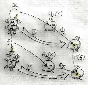
Relations between polymorphic functions

Given that Φ maps relations to relations, a universally quantified version of it:

forall A. ΦA

maps pairs of sets to pairs of values.

Now suppose that you have two polymorphic functions g and g':

g  :: forall a . φa
g' :: forall a'. ψa'

They both map types (sets) to values.

  • We can instantiate g at some type a, and it will return a value ga of the type b=φa.
  • We can instantiate g' at some type a', and it will return a value g'a' of the type b'=ψa'.

We can do this for any relation A between two arbitrary sets a and a'.

We will say that g and g' are related through the relation induced by the type (forall A. ΦA) iff the results ga and g'a' are related by ΦA.

PolyFunRel

Fig 3. Relation between two polymorphic functions. The pair (g a, g' a') falls inside the relation ΦA.

In other words, polymorphic functions are related if they map related types to related values. Notice that in the interesting examples these values are themselves functions.

With these definitions, we can now reinterpret any type signature as a relation between values.

The Parametricity Theorem

Reynolds’ second key insight was that any term is in a relation with itself — the relation being induced by the term’s type. We have indeed defined the mapping of types to relations to make this work. Primitive types turn into identity relations, so obviously a primitive value is in relation with itself. A function between primitive types is in relation with itself because it maps related (equal) arguments into related (equal) results. A list or a pair of primitive types is in relation with itself because each element of it is equal to itself. You can recurse and consider a list of functions, or a pair of lists, etc., building the proof inductively, proceeding from simpler types to more and more complex types. The proof goes over all possible term construction rules and typing rules in a given theory.

Formally, this kind of proof is called “structural induction,” because you’re showing that more complex structures will satisfy the theorem as long as the simpler ones, from which they are constructed, do. The only tricky part is dealing with polymorphic functions, because they are quantified over all types (including polymorphic types). In fact, this is the reason why the naive interpretation of types as sets breaks down (see, however, Pitts’ paper). It is possible, however, to prove the parametricity theorem in a more general setting, for instance, using frames, or in the framework of operational semantics, so we won’t worry about it here.

Wadler’s key insight was to interpret Reynolds’ theorem not only as a way of identifying different implementations of the same type — for instance, cartesian and polar representations of complex numbers — but also as a source of free theorems for polymorphic types.

Let’s try applying parametricity theorem to some simple examples. Take a constant term: an integer like 5. Its type Int can be interpreted as a relation, which we defined to be the identity relation (it’s one of the primitive types). And indeed, 5 is in this relation with 5.

Take a function like:

ord :: Char -> Int

Its type defines a relation between functions: Two functions of the type Char->Int are related if they return equal integers for equal characters. Obviously, ord is in this relation with itself.

Parametricity in Action

Those were trivial examples. The interesting ones involve polymorphic functions. So let’s go back to our starting example. The term now is the polymorphic function r whose type is:

r :: forall a . [a] -> [a]

Parametricity tells us that r is in relation with itself. However, comparing a polymorphic function to itself involves comparing the instantiations of the same function at two arbitrary types, say a and a'. Let’s go through this example step by step.

We are free to pick an arbitrary relation A between elements of two arbitrary input sets a and a'. The type of r induces a mapping Φ on relations. As with every function on relations, we have to first identify the two type constructors φ and ψ, one mapping a and one mapping a'. In our case they are identical, because they are induced by the same polymorphic function. They are equal to:

Λ a. [a]->[a]

It’s a type constructor that maps an arbitrary type a to the function type [a]->[a].

The universal quantifier forall means that r lets us pick a particular value of the type [a]->[a] for each a. This value is a function that we call ra. We don’t care how this function is picked by r, as long as it’s picked uniformly, using a single formula for all a, so that our parametricity theorem holds.

FreeTheorem

Fig 4. Polymorphic function r maps related types to related values, which themselves are functions on lists

Parametricity means that, if a is related to a', then:

ra <=> ra'

This particular relation is induced by the function type [a]->[a]. By our definition, two functions are related if they map related arguments to related results. In this case both the arguments and the results are lists. So if we have two related lists, as and as':

as  :: [a]
as' :: [a']

they must, by parametricity, be mapped to two related lists, bs and bs':

bs  = ra  as
bs' = ra' as'

This must be true for any relation A, so let’s pick a functional relation generated by some function:

f :: a -> a'

This relation induces a relation on lists:

as' = map f as

The results of applying r, therefore, must be related through the same relation:

bs' = map f bs

Combining all these equalities, we get our expected result:

ra' (map f as) = map f (ra as)

Parametricity and Natural Transformations

The free theorem I used as the running example is interesting for another reason: The list constructor is a functor. You may think of functors as generalized containers for storing arbitrary types of values. You can imagine that they have shapes; and for two containers of the same shape you may establish a correspondence between “positions” at which the elements are stored. This is quite easy for traditional containers like lists or trees, and with a leap of faith it can be stretched to non-traditional “containers” like functions. We used the intuition of relations corresponding to the idea of “occupying the same position” within a data structure. This notion can be readily generalized to any polymorphic containers. Two trees, for instance, are related if they are both empty, or if they have the same shape and their corresponding elements are related.

Let’s try another functor: You can also think of Maybe as having two shapes: Nothing and Just. Two Nothings are always related, and two Justs are related if their contents are related.

This observation immediately gives us a free theorem about polymorphic functions of the type:

r :: forall a. [a] -> Maybe a

an example of which is safeHead. The theorem is:

fmap h . safeHead == safeHead . fmap h

Notice that the fmap on the left is defined by the Maybe functor, whereas the one on the right is the list one.

If you accept the premise that an appropriate relation can be defined for any functor, then you can derive a free theorem for all polymorphic functions of the type:

r :: forall a. f a -> g a

where f and g are functors. This type of function is known as a natural transformation between the two functors, and the free theorem:

fmap h . r == r . fmap h

is the naturality condition. That’s how naturality follows from parametricity.

Acknowledgments

I’d like to thank all the people I talked to about parametricity at the ICFP in Gothenburg, and Edward Kmett for reading and commenting on the draft of this blog.

Appendix 1: Other Examples

Here’s a list of other free theorems from Wadler’s paper. You might try proving them using parametricity.

r :: [a] -> a -- for instance, head
f . r == r . fmap f
r :: [a] -> [a] -> [a] -- for instance, (++)
fmap f (r as bs) == r (fmap f as) (fmap f bs)
r :: [[a]] -> [a] -- for instance, concat
fmap f . r == r . fmap (fmap f)
r :: (a, b) -> a -- for instance, fst
f . r == r . mapPair (f, g)
r :: (a, b) -> b -- for instance, snd
g . r == r . mapPair (f, g)
r :: ([a], [b]) -> [(a, b)] -- for instance, uncurry zip
fmap (mapPair (f, g)) . r == r . mapPair (fmap f, fmap g)
r :: (a -> Bool) -> [a] -> [a] -- for instance, filter
fmap f . r (p . f) = r p . fmap f
r :: (a -> a -> Ordering) -> [a] -> [a] -- for instance, sortBy
 -- assuming: f is monotone (preserves order)
fmap f . r cmp == r cmp' . fmap f
r :: (a -> b -> b) -> b -> [a] -> b -- for instance, foldl
-- assuming: g (acc x y) == acc (f x) (g y)
g . foldl acc zero == foldl acc (g zero) . fmap f
r :: a -> a -- id
f . r == r . f
r :: a -> b -> a -- for instance, the K combinator
f (r x y) == r (f x) (g y)

where:

mapPair :: (a -> c, b -> d) -> (a, b) -> (c, d)
mapPair (f, g) (x, y) = (f x, g y)

Appendix 2: Identity Function

Let’s prove that there is only one polymorphic function of the type:

r :: forall a. a -> a

and it’s the identity function:

id x = x

We start by picking a particular relation. It’s a relation between the unit type () and an arbitrary (inhabited) type a. The relation consists of just one pair ((), c), where () is the unit value and c is an element of a. By parametricity, the function

r() :: () -> ()

must be related to the function

ra :: a -> a

There is only one function of the type ()->() and it’s id(). Related functions must map related argument to related values. We know that r() maps unit value () to unit value (). Therefore ra must map c to c. Since c is arbitrary, ra must be an identity for all (inhabited) as.

Bibliography

  1. John C Reynolds, Types, Abstraction and Parametric Polymorphism
  2. Philip Wadler, Theorems for Free!
  3. Claudio Hermida, Uday S. Reddy, Edmund P. Robinson, Logical Relations and Parametricity – A Reynolds Programme for Category Theory and Programming Languages
  4. Derek Dreyer, Paremetricity and Relational Reasoning, Oregon Programming Languages Summer School
  5. Janis Voigtländer, Free Theorems Involving Type Constructor Classes

C++ is like an oil tanker — it takes a long time for it to change course. The turbulent reefs towards which C++ has been heading were spotted on the horizon more than ten years ago. I’m talking, of course, about the end of smooth sailing under the Moore’s law and the arrival of the Multicore. It took six years to acknowledge the existence of concurrency in the C++11 Standard, but that’s only the beginning. It’s becoming more and more obvious that a major paradigm shift is needed if C++ is to remain relevant in the new era.

Why do we need a new paradigm to deal with concurrency? Can’t we use object oriented programming with small modifications? The answer to this question goes to the heart of programming: it’s about composability. We humans solve complex problems by splitting them into smaller subproblems. This is a recursive process, we split subproblems into still smaller pieces, and so on. Eventually we reach the size of the problem which can be easily translated into computer code. We then have to compose all these partial solutions into larger programs.

The key to composability is being able to hide complexity at each level. This is why object oriented programming has been so successful. When you’re implementing an object, you have to deal with its internals, with state transitions, intermediate states, etc. But once the object is implemented, all you see is the interface. The interface must be simpler than the implementation for object oriented programming to make sense. You compose larger objects from smaller objects based on their interfaces, not the details of their implementation. That’s how object oriented programming solves the problem of complexity.

Unfortunately, objects don’t compose in the presence of concurrency. They hide the wrong kind of things. They hide sharing and mutation. Let me quote the definition of data race: Two or more threads accessing the same piece of memory at the same time, at least one of them writing. In other words: Sharing + Mutation = Data Race. Nothing in the object’s interface informs you about the possibility of sharing and mutation inside the object’s implementation. Each object in isolation may be data-race-free but their composition may inadvertently introduce data races. And you won’t know about it unless you study the details of their implementation down to every single memory access.

In Java, an attempt had been made to mollify this problem: Every object is equipped with a mutex that can be invoked by declaring the method synchronized. This is not a scalable solution. Even Java’s clever thin lock implementation incurs non-negligible performance overhead, so it is used only when the programmer is well aware of potential races, which requires deep insight into the implementation of all subobjects, exactly the thing we are trying to avoid.

More importantly, locking itself doesn’t compose. There’s a classic example of a locked bank account whose deposit and withdraw methods are synchronized by a lock. The problem occurs when one tries to transfer money from one account to another. Without exposing the locks, it’s impossible to avoid a transient state in which the funds have already left one account but haven’t reached the second. With locks exposed, one may try to hold both locks during the transfer, but that creates a real potential for deadlocks. (Software Transactional Memory provides a composable solution to this problem, but there are no practical implementations of STM outside of Haskell and Clojure.)

Moreover, if we are interested in taking advantage of multicores to improve performance, the use of locks is a non-starter. Eking out parallel performance is hard enough without locks, given all the overheads of thread management and the Amdahl’s law. Parallelism requires a drastically different approach.

Since the central problem of concurrency is the conflict between sharing and mutation, the solution is to control these two aspects of programming. We can do mutation to our heart’s content as long as there’s no sharing. For instance, we can mutate local variables; or we can ensure unique ownership by making deep copies, using move semantics, or by employing unique_ptrs. Unique ownership plays very important role in message passing, allowing large amounts of data to be passed cheaply between threads.

However, the key to multicore programming is controlling mutation. This is why functional languages have been steadily gaining ground in concurrency and parallelism. In a nutshell, functional programmers have found a way to program using what, to all intents and purposes, looks like immutable data. An imperative programmer, when faced with immutability, is as confused as a barbecue cook in a vegetarian kitchen. And the truth is that virtually all data structures from the C++ standard library are unsuitable for this kind of programming — the standard vector being the worst offender. A continuous slab of memory is perfect for random or sequential access, but the moment mutation is involved, you can’t share it between threads. Of course, you can use a mutex to lock the whole vector every time you access it, but as I explained already, you can forget about performance and composability of such a solution.

The trick with functional data structures is that they appear immutable, and therefore require no synchronization when accessed from multiple threads. Mutation is replaced by construction: you construct a new object that’s a clone of the source object but with the requested modification in place. Obviously, if you tried to do this with a vector, you’d end up with a lot of copying. But functional data structures are designed for maximum sharing of representation. So a clone of a functional object will share most of its data with the original, and only record a small delta. The sharing is totally transparent since the originals are guaranteed to be immutable.

A singly-linked list is a classical, if not somewhat trivial, example of such a data structure. Adding an element to the front of a list requires only the creation of a single node to store the new value and a pointer to the original (immutable) list. There are also many tree-like data structures that are logarithmically cheap to clone-mutate (red-black trees, leftist heaps). Parallel algorithms are easy to implement with functional data structures, since the programmer doesn’t have to worry about synchronization.

Functional data structures, also known as “persistent” data structures, are naturally composable. This follows from the composability of immutable data — you can build larger immutable objects from smaller immutable objects. But there’s more to it: This new way of mutating by construction also composes well. A composite persistent object can be clone-mutated by clone-mutating only the objects on the path to the mutation; everything else can be safely shared.

Concurrency also introduces nonstandard flows of control. In general, things don’t progress sequentially. Programmers have to deal with inversion of control, jumping from handler to handler, keeping track of shared mutable state, etc. Again, in functional programming this is nothing unusual. Functions are first class citizens and they can be composed in many ways. A handler is nothing but a continuation in the continuation passing style. Continuations do compose, albeit in ways that are not familiar to imperative programmers. Functional programmers have a powerful compositional tool called a monad that, among other things, can linearize inverted flow of control. The design of libraries for concurrent programming makes much more sense once you understand that.

A paradigm shift towards functional programming is unavoidable and I’m glad to report that there’s a growing awareness of that new trend among C++ programmers. I used to be the odd guy talking about Haskell and monads at C++ meetings and conferences. This is no longer so. There was a sea change at this year’s C++Now. The cool kids were all talking about functional programming, and the presentation “Functional Data Structures in C++” earned me the most inspiring session award. I take it as a sign that the C++ community is ready for a big change.


Lazy evaluation can be a powerful tool for structuring your code. For instance, it can let you turn your code inside out, inverting the flow of control. Many a Haskell program take advantage of laziness to express algorithms in clear succinct terms, turning them from recipes to declarations.

The question for today’s blog post is: How can we tap the power of lazy evaluation in an inherently eager language like C++? I’ll lead you through a simple coding example and gradually introduce the building blocks of lazy programming: the suspension, the lazy stream, and a whole slew of functional algorithms that let you operate on them. In the process we’ll discover some fundamental functional patterns like functors, monads, and monoids. I have discussed them already in my post about C++ futures. It’s very edifying to see them emerge in a completely different context.

The Problem

Let’s write a program that prints the first n Pythagorean triples. A Pythagorean triple consists of three integers, x, y, and z, that satisfy the relation x2 + y2 = z2. Let’s not be fancy and just go with the brute force approach. Here’s the program in C:

void printNTriples(int n)
{
    int i = 0;
    for (int z = 1; ; ++z)
        for (int x = 1; x <= z; ++x)
            for (int y = x; y <= z; ++y)
                if (x*x + y*y == z*z) {
                    printf("%d, %d, %d\n", x, y, z);
                    if (++i == n)
                        return;
                }
}

Here, a single C function serves three distinct purposes: It

  1. Generates Pythagorean triples,
  2. Prints them,
  3. Counts them; and when the count reaches n, breaks.

This is fine, as long as you don’t have to modify or reuse this code. But what if, for instance, instead of printing, you wanted to draw the triples as triangles? Or if you wanted to stop as soon as one of the numbers reached 100? The problem with this code is that it’s structured inside out: both the test and the sink for data are embedded in the innermost loop of the algorithm. A more natural and flexible approach would be to:

  1. Generate the list of Pythagorean triples,
  2. Take the first ten of them, and
  3. Print them.

And that’s exactly how you’d write this program in Haskell:

main = print (take 10 triples)

triples = [(x, y, z) | z <- [1..]
                     , x <- [1..z]
                     , y <- [x..z]
                     , x^2 + y^2 == z^2]

This program reads: take 10 triples and print them. It declares triples as a list (square brackets mean a list) of triples (x, y, z), where (the vertical bar reads “where”) z is an element of the list of integers from 1 to infinity, x is from 1 to z, y is from x to z, and the sum of squares of x and y is equal to the square of z. This notation is called “list comprehension” and is characteristic of Haskell terseness.

You see the difference? Haskell let’s you abstract the notion of the list of Pythagorean triples so you can operate on it as one entity, whereas in C (or, for that matter, in C++) we were not able to disentangle the different, orthogonal, aspects of the program.

The key advantage of Haskell in this case is its ability to deal with infinite lists. And this ability comes from Haskell’s inherent laziness. Things are never evaluated in Haskell until they are absolutely needed. In the program above, it was the call to print that forced Haskell to actually do some work: take 10 elements from the list of triples. Since the triples weren’t there yet, it had to calculate them, but only as many as were requested and not a number more.

Suspension

We’ll start with the most basic building block of laziness: a suspended function. Here’s the first naive attempt:

template<class T>
class Susp {
public:
    explicit Susp(std::function<T()> f)
        : _f(f)
    {}
    T get() { return _f(); }
private:
    std::function<T()> _f;
};

We often create suspensions using lambda functions, as in:

int x = 2;
int y = 3;
Susp<int> sum([x, y]() { return x + y; });
...
int z = sum.get();

Notice that the suspended lambda may capture variables from its environment: here x and y. A lambda, and therefore a suspension, is a closure.

The trouble with this implementation is that the function is re-executed every time we call get. There are several problems with that: If the function is not pure, we may get different values each time; if the function has side effects, these may happen multiple times; and if the function is expensive, the performance will suffer. All these problems may be addressed by memoizing the value.

Here’s the idea: The first time the client calls get we should execute the function and store the returned value in a member variable. Subsequent calls should go directly to that variable. We could implement this by setting a Boolean flag on the first call and then checking it on every subsequent call, but there’s a better implementation that uses thunks.

A thunk is a pointer to a free function taking a suspension (the this pointer) and returning a value (by const reference). The get method simply calls this thunk, passing it the this pointer.

Initially, the thunk is set to thunkForce, which calls the method setMemo. This method evaluates the function, stores the result in _memo, switches the thunk to thunkGet, and returns the memoized value. On subsequent calls get goes through the getMemo thunk which simply returns the memoized value.

template<class T>
class Susp
{
    // thunk
    static T const & thunkForce(Susp * susp) {
        return susp->setMemo();
    }
    // thunk
    static T const & thunkGet(Susp * susp) {
        return susp->getMemo();
    }
    T const & getMemo() {
        return _memo;
    }
    T const & setMemo() {
        _memo = _f();
        _thunk = &thunkGet;
        return getMemo();
    }
public:
    explicit Susp(std::function<T()> f)
        : _f(f), _thunk(&thunkForce), _memo(T())
    {}
    T const & get() {
        return _thunk(this);
    }
private:
    T const & (*_thunk)(Susp *);
    mutable T   _memo;

    std::function<T()> _f;
};

(By the way, the function pointer declaration of _thunk looks pretty scary in C++, doesn’t it?)

[Edit: I decided to remove the discussion of the thread safe implementation since it wasn’t ready for publication. The current implementation is not thread safe.]

You can find a lot more detail about the Haskell implementation of suspended functions in the paper by Tim Harris, Simon Marlow, and Simon Peyton Jones, Haskell on a Shared-Memory Multiprocessor.

Lazy Stream

The loop we used to produce Pythagorean triples in C worked on the push principle — data was pushed towards the sink. If we want to deal with infinite lists, we have to use the pull principle. It should be up to the client to control the flow of data. That’s the inversion of control I was talking about in the introduction.

We’ll use a lazy list and call it a stream. In C++ a similar idea is sometimes expressed in terms of input and forward iterators, although it is understood that an iterator itself is not the source or the owner of data — just an interface to one. So we’ll stick with the idea of a stream.

We’ll implement the stream in the functional style as a persistent data structure fashioned after persistent lists (see my series of blog post on persistent data structures). It means that a stream, once constructed, is never modified. To “advance” the stream, we’ll have to create a new one by calling the const method pop_front.

Let’s start with the definition: A stream is either empty or it contains a suspended cell. This immediately suggests the implementation as a (possibly null) pointer to a cell. Since the whole stream is immutable, the cell will be immutable too, so it’s perfectly safe to share it between copies of the stream. We can therefore use a shared pointer:

template<class T>
class Stream
{
private:
    std::shared_ptr <Susp<Cell<T>>> _lazyCell;
};

Of course, because of reference counting and memoization, the stream is only conceptually immutable and, in the current implementation, not thread safe.

So what’s in the Cell? Remember, we want to be able to generate infinite sequences, so Stream must contain the DNA for not only producing the value of type T but also for producing the offspring — another (lazy) Stream of values. The Cell is just that: A value and a stream.

template<class T>
class Cell
{
public:
    Cell() {} // need default constructor for memoization
    Cell(T v, Stream<T> const & tail)
        : _v(v), _tail(tail)
    {}
    explicit Cell(T v) : _v(v) {}
    T val() const {
        return _v;
    }
    Stream<T> pop_front() const {
        return _tail;
    }
private:
    T _v;
    Stream<T> _tail;
};

This mutually recursive pair of data structures works together amazingly well.

template<class T>
class Stream
{
private:
    std::shared_ptr <Susp<Cell<T>>> _lazyCell;
public:
    Stream() {}
    Stream(std::function<Cell<T>()> f)
        : _lazyCell(std::make_shared<Susp<Cell<T>>>(f))
    {}
    Stream(Stream && stm)
        : _lazyCell(std::move(stm._lazyCell))
    {}
    Stream & operator=(Stream && stm)
    {
        _lazyCell = std::move(stm._lazyCell);
        return *this;
    }
    bool isEmpty() const
    {
        return !_lazyCell;
    }
    T get() const
    {
        return _lazyCell->get().val();
    }
    Stream<T> pop_front() const
    {
        return _lazyCell->get().pop_front();
    }
};

There are several things worth pointing out. The two constructors follow our formal definition of the Stream: one constructs an empty stream, the other constructs a suspended Cell. A suspension is created from a function returning Cell.

I also added a move constructor and a move assignment operator for efficiency. We’ll see it used in the implementation of forEach.

The magic happens when we call get for the first time. That’s when the suspended Cell comes to life. The value and the new stream are produced and memoized for later use. Or, this may happen if the first call is to pop_front. Notice that pop_front is a const method — the Stream itself is immutable. The method returns a new stream that encapsulates the rest of the sequence.

Let’s get our feet wet by constructing a stream of integers from n to infinity. The constructor of a Stream takes a function that returns a Cell. We’ll use a lambda that captures the value of n. It creates a Cell with that value and a tail, which it obtains by calling intsFrom with n+1:

Stream<int> intsFrom(int n)
{
    return Stream<int>([n]()
    {
        return Cell<int>(n, intsFrom(n + 1)); 
    });
}

It’s a recursive definition, but without the usual recursive function calls that eat up the stack. The call to the inner intsFrom is not made from the outer intsFrom. Instead it’s made the first time get is called on the emerging Stream.

Of course, we can also create finite streams, like this one, which produces integers from n to m:

Stream<int> ints(int n, int m)
{
    if (n > m)
        return Stream<int>();
    return Stream<int>([n, m]()
    {
        return Cell<int>(n, ints(n + 1, m));
    });
}

The trick is to capture the limit m as well as the recursion variable n. When the limit is reached, we simply return an empty Stream.

We’ll also need the method take, which creates a Stream containing the first n elements of the original stream:

Stream take(int n) const {
    if (n == 0 || isEmpty())
        return Stream();
    auto cell = _lazyCell;
    return Stream([cell, n]()
    {
        auto v = cell->get().val();
        auto t = cell->get().pop_front();
        return Cell<T>(v, t.take(n - 1));
    });
}

Here we are capturing the suspended cell and use it to lazily generate the elements of the new, truncated, Stream. Again, the key to understanding why this works is to keep in mind that Streams and Cells are conceptually immutable, and therefore can be shared by the implementation. This has some interesting side effects, which don’t influence the results, but change the performance. For instance, if the caller of take forces the evaluation of the first n elements — e.g., by passing them through the consuming forEach below — these elements will appear miraculously memoized in the original Stream.

Finally, we’ll need some way to iterate through streams. Here’s an implementation of forEach that consumes the stream while enumerating it and feeding its elements to a function.

template<class T, class F>
void forEach(Stream<T> strm, F f)
{
    while (!strm.isEmpty())
    {
        f(strm.get());
        strm = strm.pop_front();
    }
}

It’s the assignment:

strm = strm.pop_front();

which consumes the stream by decreasing the reference count of the head of the Stream. In particular, if you pass an rvalue Stream to forEach, its elements will be generated and deleted in lockstep. The algorithm will use constant memory, independent of the virtual length of the Stream. What Haskell accomplishes with garbage collection, we approximate in C++ with reference counting and shared_ptr.

Working with Streams

It’s not immediately obvious how to translate our Pythagorean triple program from nested loops to lazy streams, so we’ll have to take inspiration from the corresponding Haskell program. Let me first rewrite it using a slightly different notation:

triples = do
    z <- [1..]
    x <- [1..z]
    y <- [x..z]
    guard (x^2 + y^2 == z^2)
    return (x, y, z)

The general idea is this: Start with the stream of integers from 1 to infinity. For every such integer — call it z — create a stream from 1 to z. For each of those — call them x — create a stream from x to z. Filter out those which don’t satisfy the Pythagorean constraint. Finally, output a stream of tuples (x, y, z).

So far we’ve learned how to create a stream of integers — we have the function intsFrom. But now we’ll have to do something for each of these integers. We can’t just enumerate those integers and apply a function to each, because that would take us eternity. So we need a way to act on each element of a stream lazily.

In functional programming this is called mapping a function over a list. In general, a parameterized data structure that can be mapped over is called a functor. I’m going to show you that our Stream is a functor.

Stream as a Functor

The idea is simple: we want to apply a function to each element of a stream to get a new transformed stream (it’s very similar to the std::transform algorithm from STL). The catch is: We want to do it generically and lazily.

To make the algorithm — we’ll call it fmap — generic, we have to parameterize it over types. The algorithm starts with a Stream of elements of type T and a function from T to some other type U. The result should be a stream of U.

We don’t want to make U the template argument, because then the client would have to specify it explicitly. We want the compiler to deduce this type from the type of the function. We want, therefore, the function type F to be the parameter of our template (this will also allow us to call it uniformly with function pointers, function objects, and lambdas):

template<class T, class F>
auto fmap(Stream<T> stm, F f)

Without the use of concepts, we have no way of enforcing, or even specifying, that F be a type of a function from T to U. The best we can do is to statically assert it inside the function:

static_assert(std::is_convertible<F, std::function<U(T)>>::value,
        "fmap requires a function type U(T)");

But what is U? We can get at it using decltype:

decltype(f(stm.get()));

Notice that decltype takes, as an argument, an expression that can be statically typed. Here, the expression is a function call of f. We also need a dummy argument for this function: we use the result of stm.get(). The argument to decltype is never evaluated, but it is type-checked at compile time.

One final problem is how to specify the return type of fmap. It’s supposed to be Stream<U>, but we don’t know U until we apply decltype to the arguments of fmap. We have to use the new auto function declaration syntax of C++11. So here are all the type-related preliminaries:

template<class T, class F>
auto fmap(Stream<T> stm, F f)->Stream<decltype(f(stm.get()))>
{
    using U = decltype(f(stm.get()));
    static_assert(std::is_convertible<F, std::function<U(T)>>::value,
        "fmap requires a function type U(T)");
    ...
}

Compared to that, the actual implementation of fmap seems rather straightforward:

    if (stm.isEmpty()) return Stream<U>();
    return Stream<U>([stm, f]()
    {
        return Cell<U>(f(stm.get()), fmap(stm.pop_front(), f));
    });

In words: If the stream is empty, we’re done — return an empty stream. Otherwise, create a new stream by suspending a lambda function. That function captures the original stream (by value) and the function f, and returns a Cell. That cell contains the value of f acting on the first element of the original stream, and a tail. The tail is created with fmap acting on the rest of the original stream.

Equipped with fmap, we can now attempt to take the first step towards generating our triples: apply the function ints(1, z) to each element of the stream intsFrom(1):

fmap(intsFrom(1), [](int z)
{
    return ints(1, z);
});

The result is a Stream of Streams of integers of the shape:

1
1 2
1 2 3
1 2 3 4
1 2 3 4 5
...

But now we are stuck. We’d like to apply ints(x, z) to each element of that sequence, but we don’t know how to get through two levels of Stream. Our fmap can only get through one layer. We need a way to flatten a Stream of Streams. That functionality is part of what functional programmers call a monad. So let me show you that Stream is indeed a monad.

Stream as a Monad

If you think of a Stream as a list, the flattening of a list of lists is just concatenation. Suppose for a moment that we know how to lazily concatenate two Streams (we’ll get to it later) and let’s implement a function mjoin that concatenates a whole Stream of Streams.

You might have noticed a pattern in the implementation of lazy functions on streams. We use some kind of recursion, which starts with “Are we done yet?” If not, we do an operation that involves one element of the stream and the result of a recursive call to the function itself.

The “Are we done yet?” question usually involves testing for an empty stream. But here we are dealing with a Stream of Streams, so we have to test two levels deep. This way we’ll ensure that the concatenation of a Stream of empty Streams immediately returns an empty Stream.

The recursive step in mjoin creates a Cell whose element is the head of the first stream, and whose tail is the concatenation of the tail of the first stream and the result of mjoin of the rest of the streams:

template<class T>
Stream<T> mjoin(Stream<Stream<T>> stm)
{
    while (!stm.isEmpty() && stm.get().isEmpty())
    {
        stm = stm.pop_front();
    }
    if (stm.isEmpty()) return Stream<T>();
    return Stream<T>([stm]()
    {
        Stream<T> hd = stm.get();
        return Cell<T>( hd.get()
                      , concat(hd.pop_front(), mjoin(stm.pop_front())));
    });
}

The combination of fmap and mjoin lets us compose function like intsFrom or ints that return Streams. In fact, this combination is so common that it deserves its own function, which we’ll call mbind:

template<class T, class F>
auto mbind(Stream<T> stm, F f) -> decltype(f(stm.get()))
{
    return mjoin(fmap(stm, f));
}

If we use mbind in place of fmap:

mbind(intsFrom(1), [](int z)
{
    return ints(1, z);
});

we can produce a flattened list:

1 1 2 1 2 3 1 2 3 4...

But it’s not just the list: Each element of the list comes with variables that are defined in its environment — here the variable z. We can keep chaining calls to mbind and capture more variables in the process:

mbind(intsFrom(1), [](int z)
{
    return mbind(ints(1, z), [z](int x)
    {
        return mbind(ints(x, z), [x, z](int y)
        {
            ...
        }
    }
}

At this point we have captured the triples x, y, z, and are ready for the Pythagorean testing. But before we do it, let’s define two additional functions that we’ll use later.

The first one is mthen which is a version of mbind that takes a function of no arguments. The idea is that such a function will be executed for each element of the stream, but it won’t use the value of that element. The important thing is that the function will not be executed when the input stream is empty. In that case, mthen will return an empty stream.

We implement mthen using a slightly modified version of fmap that takes a function f of no arguments:

template<class T, class F>
auto fmapv(Stream<T> stm, F f)->Stream<decltype(f())>
{
    using U = decltype(f());
    static_assert(std::is_convertible<F, std::function<U()>>::value,
        "fmapv requires a function type U()");

    if (stm.isEmpty()) return Stream<U>();
    return Stream<U>([stm, f]()
    {
        return Cell<U>(f(), fmapv(stm.pop_front(), f));
    });
}

We plug it into the definition of mthen the same way fmap was used in mbind:

template<class T, class F>
auto mthen(Stream<T> stm, F f) -> decltype(f())
{
    return mjoin(fmapv(stm, f));
}

The second useful function is mreturn, which simply turns a value of any type into a one-element Stream:

template<class T>
Stream<T> mreturn(T v)
{
    return Stream<T>([v]() {
        return Cell<T>(v);
    });
}

We’ll need mreturn to turn our triples into Streams.

It so happens that a parameterized type equipped with mbind and mreturn is called a monad (it must also satisfy some additional monadic laws, which I won’t talk about here). Our lazy Stream is indeed a monad.

Stream as a Monoid and a Monad Plus

When implementing mjoin we used the function concat to lazily concatenate two Streams. Its implementation follows the same recursive pattern we’ve seen so many times:

template<class T>
Stream<T> concat( Stream<T> lft
                , Stream<T> rgt)
{
    if (lft.isEmpty())
        return rgt;
    return Stream<T>([=]()
    {
        return Cell<T>(lft.get(), concat<T>(lft.pop_front(), rgt));
    });
}

What’s interesting is that the concatenation of streams puts them under yet another well known functional pattern: a monoid. A monoid is equipped with a binary operation, just like concat, which must be associative and possess a unit element. It’s easy to convince yourself that concatenation of Streams is indeed associative, and that the neutral element is an empty Stream. Concatenating an empty Stream, whether in front or in the back of any other Stream, doesn’t change the original Stream.

What’s even more interesting is that being a combination of a monoid and a monad makes Stream into a monad plus, and every monad plus defines a guard function — exactly what we need for the filtering of our triples. This function takes a Boolean argument and outputs a Stream. If the Boolean is false, the Stream is empty (the unit element of monad plus!), otherwise it’s a singleton Stream. We really don’t care what value sits in this Stream — we never use the result of guard for anything but the flow of control. In Haskell, there is a special “unit” value () — here I use a nullptr as its closest C++ analog.

Stream<void*> guard(bool b)
{
    if (b) return Stream<void*>(nullptr);
    else return Stream<void*>();
}

We can now pipe the result of guard into mthen, which will ignore the content of the Stream but won’t fire when the Stream is empty. When the Stream is not empty, we will call mreturn to output a singleton Stream with the result tuple:

Stream<std::tuple<int, int, int>> triples()
{
    return mbind(intsFrom(1), [](int z)
    {
        return mbind(ints(1, z), [z](int x)
        {
            return mbind(ints(x, z), [x, z](int y)
            {
                return mthen(guard(x*x + y*y == z*z), [x, y, z]()
                {
                    return mreturn(std::make_tuple(x, y, z));
                });
            });
        });
    });
}

These singletons will then be concatenated by the three levels of mbind to create one continuous lazy Stream of Pythagorean triples.

Compare this function with its Haskell counterpart:

triples = do
    z <- [1..]
    x <- [1..z]
    y <- [x..z]
    guard (x^2 + y^2 == z^2)
    return (x, y, z)

Now, the client can take 10 of those triples from the Stream — and the triples still won’t be evaluated!. It’s the consuming forEach that finally forces the evaluation:

void test()
{
    auto strm = triples().take(10);
    forEach(std::move(strm), [](std::tuple<int, int, int> const & t)
    {
        std::cout << std::get<0>(t) << ", " 
                  << std::get<1>(t) << ", " 
                  << std::get<2>(t) << std::endl;
    });
}

Conclusion

The generation of Pythagorean triples is a toy example, but it shows how lazy evaluation can be used to restructure code in order to make it more reusable. You can use the same function triples to print the values in one part of your program and draw triangles in another. You can filter the triples or impose different termination conditions. You can use the same trick to generate an infinite set of approximation to the solution of a numerical problem, and then use different strategies to truncate it. Or you can create an infinite set of animation frames, and so on.

The building blocks of laziness are also reusable. I have used them to implement the solution to the eight-queen problem and a conference scheduling program. Once they made thread safe, the combinators that bind them are thread safe too. This is, in general, the property of persistent data structures.

You might be concerned about the performance of lazy data structures, and rightly so. They use the heap heavily, so memory allocation and deallocation is a serious performance bottleneck. There are many situation, though, where code structure, reusability, maintenance, and correctness (especially in multithreaded code) are more important than performance. And there are some problems that might be extremely hard to express without the additional flexibility gained from laziness.

I made the sources to all code in this post available on GitHub.


[If you prefer, you may watch the video of my talk on this topic (here are the slides).]

If you thought you were safe from functional programming in your cozy C++ niche, think again! First the lambdas and function objects and now the monad camouflaged as std::future. But do not despair, it’s all just patterns. You won’t find them in the Gang of Four book, but once you see them, they will become obvious.

Let me give you some background: I was very disappointed with the design of C++11 std::future. I described my misgivings in: Broken Promises — C++0x futures. I also made a few suggestions as how to fix it: Futures Done Right. Five years went by and, lo and behold, a proposal to improve std::future and related API, N3721, was presented to the Standards Committee for discussion. I thought it would be a no brainer, since the proposal was fixing obvious holes in the original design. A week ago I attended the meetings of the C++ Standards Committee in Issaquah — since it was within driving distance from me — and was I in for a surprise! Apparently some design patterns that form the foundation of functional programming are not obvious to everybody. So now I find myself on the other side of the discussion and will try to explain why the improved design of std::future is right.

Design arguments are not easy. You can’t mathematically prove that one design is better than another, or a certain set of abstractions is better than another — unless you discover some obvious design flaws in one of them. You might have a gut feeling that a particular solution is elegant, but how do you argue about elegance?

Thankfully, when designing a library, there are some well known and accepted criteria. The most important ones, in my mind, are orthogonality, a.k.a., separation of concerns, and composability. It also helps if the solution has been previously implemented and tested, especially in more than one language. I will argue that this is indeed the case with the extended std::future design. In the process, I will describe some programming patterns that might be new to C++ programmers but have been tried and tested in functional languages. They tend to pop up more and more in imperative languages, especially in connection with concurrency and parallelism.

The Problem

In a nutshell, the problem that std::future is trying to solve is that of returning the result of a computation that’s being performed in parallel, or returning the result of an asynchronous call. For instance, you start a computation in a separate thread (or a more general execution agent) and you want to, at some point in time, get back the result of that computation. This is one of the simplest models of concurrency: delegating the execution of a function (a closure) to another thread.

To return a value from one thread to another you need some kind of a communication channel. One thread puts a value in the channel, another picks it up. Instead of providing one channel abstraction, as does ML or Haskell, C++11 splits it into two separate abstractions: the promise and the future. The promise is the push end of the channel, the future is the pull end. (In Rust there are similar objects called Chan and Port.)

The general pattern is for the client to construct a promise, get the future from it using get_future, and start a thread, passing it the promise. When the thread is done, it puts the result in the promise using set_value. In the meanwhile, the calling thread may do some other work and eventually decide to retrieve the result from the future by calling its method get. If the promise has been fulfilled, get returns immediately with the value, otherwise it blocks until the value is available.

This pattern involves some boilerplate code dealing with the promise side of things, so the Standard introduced a shortcut called std::async to simplify it. You call std::async with a plain function (closure) and its result is automatically put into a hidden promise. All the client sees is the future side of the channel. (I am simplifying things by ignoring exception handling and various modes of starting async.)

The Functor Pattern

Here’s the first abstraction: A future is an object that encapsulates a value. By itself, this would be a pretty useless abstraction unless the encapsulation came with some other functionality or restriction. For instance, std::unique_ptr encapsulates a value, but also manages the lifetime of the memory it occupies. A future encapsulates a value, but you might have to block to get it. Functional languages have a very useful pattern for just this kind of situation: the functor pattern (not to be confused with the C++ misnomer for a function object). A functor encapsulates a value of an arbitrary type, plus it lets you act on it with a function.

Notice that the functor doesn’t necessarily give you access to the value — instead it lets you modify it. The beauty of it is that, in the case of a future, a functor gives you the means to modify the value that potentially isn’t there yet — and it lets you do it without blocking. Of course, behind the scenes, the function (closure) that you provide is stored in the future and only applied when the value is ready and is being accessed using get.

The first part of the fix that was proposed to the Committee was to turn std::future into a functor. Technically, this is done by adding a new method, then:

template<typename F>
auto future::then(F&& func) -> future<decltype(func(*this))>;

This method takes a function object func to be applied to the future in question. The result is a new future of the type that is returned by the function object, decltype(func(*this)).

Things are slightly muddled by the fact that a future not only encapsulates the value to be calculated but also the possibility of an exception. This is why the function passed to then takes the whole future, from which it can extract the value using get, which at that point is guaranteed not to block, but may rethrow an exception. There is an additional proposal N3865 to introduce another method, next, that would deal only with the value, not the exception. The advantage of next is that it could be called with a regular function unaware of the existence of futures, with no additional boilerplate. For simplicity, I’ll be using next in what follows.

The functor pattern makes perfect sense for composing a regular function on top of an asynchronous function (one returning a future), but it’s more general than that. Any time you have an object that is parameterized by an arbitrary type, you might be dealing with a functor. In C++, that would be a template class that doesn’t impose any restrictions on its template argument. Most containers have this property. In order for a generic class to be a functor it must also support a means to operate on its contents. Most containers in STL provide this functionality through the algorithm std::transform. For an imperative programmer it might come as a surprise that such disparate things as futures and containers fall under the same functional pattern — a functor.

Unlike in functional languages, in C++ there is no natural reusable expression for the functor pattern, so it’s more of the pattern in the head of the programmer. For instance, because of memory management considerations, std::transform operates on iterators rather than containers — the storage for the target container must be either pre-allocated or allocated on demand through iterator adapters. One could try to provide iterator adapters for futures, so they could be operated on by std::transform, but ultimately the transformation has to act on the internals of the future (i.e., store the function object in it) so it either has to be a method or a friend of the future.

The Monad Pattern

The functor pattern is not enough to provide full composability for futures. The likely scenario is that the user creates a library of future-returning functions, each performing a specific task. He or she then needs the means to combine such functions into more complex tasks. This is, for instance, the case when combining asynchronous operations, such as opening a file and then reading from it. Suppose we have the async_open function that returns a file handle future:

future<HANDLE> async_open(string &);

and the async_read function that takes a file handle and returns a future with the buffer filled with data:

future<Buffer> async_read(HANDLE fh);

If you combine the two using next, the result will be a future of a future:

future<future<Buffer>> ffBuf = async_open("foo").next(&async_read);

In order to continue chaining such calls without blocking — for instance to asynchronously process the buffer — you need a way to collapse the double future to a single future and then call next on it.

The collapsing method, unwrap, is another part of the extended future proposal. When called on a future<future<T>> it returns future<T>. It lets you chain asynchronous functions using next followed by unwrap.

async_open("foo").next(&async_read).unwrap().next(&async_process);

In functional programming such a collapsing function is called join. The combination next followed by unwrap (or, in Haskell, fmap followed by join) is so common that it has its own name, bind (in Haskell it’s the operator >>=). It might make sense to make bind another method of future (possibly under a different name). [Edit: In fact, the proposal (n3721) is to overload then to automatically perform unwrap whenever the result is a future of a future. This way then would also work as bind.]

There’s one more important usage pattern: a function that may execute asynchronously, but sometimes returns the result immediately. This often happens in recursive algorithms, when the recursion bottoms up. For instance, a parallel tree traversal function may spawn asynchronous tasks for traversing the children of a node, but when it reaches a leaf, it might want to return the result synchronously. Instead of writing complicated conditional code at each level, it’s easier to provide a “fake” future whose contents is immediately available — whose get method never blocks. Such fake future and the function that creates it called make_ready_future are also part of the proposal.

Together, the methods next (or then) and unwrap, and the function make_ready_future are easily recognizable by a functional programmer as forming the monad pattern (in Haskell, they would be called, respectively, fmap, join, and return). It’s a very general pattern for composing functions that return encapsulated values. Using a monad you may work with such functions directly, rather than unwrapping their results at every step. In the case of futures, this is an important issue, since the “unwrapping” means making a potentially blocking call to get and losing precious opportunities for parallelism. You want to set up as much computation up front and let the system schedule the most advantageous execution.

Combining functions using next, unwrap (or, equivalently, bind), and make_ready_future is equivalent to specifying data dependencies between computations and letting the runtime explore opportunities for parallelism between independent computations.

The Applicative Pattern

The combinators then and next are designed for linear composition: the output of one computation serves as the input for another. A more general pattern requires the combining of multiple asynchronous sources of data. In functional programming the problem would be described as applying a function to multiple arguments, hence the name “applicative” pattern. A functional programmer would take a multi-argument function and “lift” it to accept futures instead of immediate values.

As expected, in imperative programming things are a little messier. You have to create a barrier for all the input futures, retrieve the values, and then pass them to the multi-argument function or algorithm. The proposal contains a function called when_all that implements the first part of the process — the barrier. It takes either a pair of iterators to a container of futures or a variable number of futures, and returns a future that fires when all the arguments are ready. Conceptually, it performs a logical AND of all input futures.

The iterator version of when_all returns a future of a vector of futures, while the variadic version returns a future of a tuple of futures. It’s up to the client to get the resulting vector or tuple and iterate over it. Because of that, it’s not possible to directly chain the results of when_all the way then or next does it.

If you’re wondering how this kind of chaining is done in a functional language, you have to understand what partial application is. A function of many arguments doesn’t have to be applied to all of the arguments at once. You can imagine that applying it to the first argument doesn’t yield a value but rather a function on n-1 arguments. In C++11, this can be accomplished by calling std::bind, which takes a multi-parameter function and a value of the first argument, and returns a function object (a closure) that takes the remaining n-1 arguments (actually, you may pass it more than one argument at a time).

In this spirit, you could bind a multi-parameter function to a single future and get a future of a function of n-1 arguments. Then you are left with the problem of applying a future of a function to a future of an argument, and that’s exactly what the applicative pattern is all about. In Haskell, the Applicative class defines the operator <*> that applies an encapsulated function to an encapsulated value.

The Monoid Pattern

A very common pattern is to start several computations in parallel and pick the one that finishes first. This is the basis of speculative computation, where you pitch several algorithms against each other. Or you might be waiting for any of a number of asynchronous events, and attend to them as soon as they happen.

At a minimum you would expect a combinator that acts like a logical OR of two futures. A functional programmer would be immediately on the lookout for the monoid pattern. A monoid is equipped with a binary operation and a unit element. If the binary operation on futures picks the one that finishes first, what should the unit future be? A unit combined with any element must give back that same element. Therefore we need a future that would lose the race with any other future. We could call this special future “never.” Calling get on such a future would block forever.

In practice, one could slightly relax the definition of the “never” future. It would never return a result, but it could still throw an exception. A future like this could be used to implement a timeout. Pitching it against another future would either let the other future complete, or result in a timeout exception.

This is not the way the future extension proposal went, though. The proposed combinator is called when_any and it takes either a pair of iterators to a container of futures or a variable number of futures. It returns a future of either a vector or a tuple of futures. It’s up to the client to iterate over those futures and find the one (or the ones) that fired by calling is_ready on each of them.

The advantage of this approach is that the client may still write code to wait for the remaining futures to finish. The disadvantage is that the client is responsible for writing a lot of boilerplate code, which will obscure the program logic.

Performance and Programming Considerations

An objection to using futures as the main vehicle for asynchronous programming was raised in N3896: Library Foundations for Asynchronous Operations. The point it that it’s possible for an asynchronous API to have a result ready before the client had the opportunity to provide the continuation by calling then (or next). This results in unnecessary synchronization, which may negatively impact performance.

The alternative approach is to pass the continuation (the handler) directly to the asynchronous API. This is how a lot of asynchronous APIs are implemented at the lowest level anyway. The two approaches don’t exclude each other, but supporting both at the same time, as proposed in N3896, adds a lot of complexity to the programming model.

From the programmer’s perspective, the continuation passing model of N3896 is probably the hardest to use. The programming model is that of a state machine, with the client responsible for writing handlers for every transition.

Futures provide a useful abstraction by reifying the anticipated values. The programmer can write code as if the values were there. Futures also provide a common language between concurrent, parallel, and asynchronous worlds. It doesn’t matter if a value is to be evaluated by spawning a thread, creating a lightweight execution agent, or by calling an asynchronous API, as long as it’s encapsulated in a future. The compositional and expressional power of futures is well founded in major patterns of functional programming: the functor, the monad, the applicative, and the monoid.

There is another, even more attractive programming model that’s been proposed for C++, Resumable Functions, which makes asynchronous code look more like sequential code. This is based on a trick that’s well known to Haskell programmers in the form of the “do” notation. In C++, a resumable function would be chopped by the compiler into a series of continuations separated by await keywords. Instead of creating a future and calling then with a lambda function, the programmer would insert await and continue writing code as if the value were available synchronously.

Acknowledgment

I’d like to thank Artur Laksberg for reading the draft of this blog and providing useful feedback.


In my previous post I worked on stretching the intuition of what a container is. I proposed that, in Haskell, any functor may be interpreted as some kind of container, including the hard cases like the state functor or the IO functor. I also talked about natural transformations between functors as “repackaging” schemes for containers, which work without “breaking the eggs” — not looking inside the elements stored in the container. Continuing with this analogy: Algebras are like recipes for making omelets.

The intuition is that an algebra provides a way to combine elements stored inside a container. This cannot be done for arbitrary types because there is no generic notion of “combining.” So an algebra is always defined for a specific type. For instance, you can define an algebra for numbers because you know how to add or multiply them, or for strings because you can concatenate them, and so on. The way elements are combined by an algebra is in general driven by the structure of the container itself.

For example, think of an expression tree as a container.

data Expr a = Const a 
            | Add (Expr a) (Expr a) 
            | Mul (Expr a) (Expr a)

We could define many algebras for it. An integer algebra would work on an expression tree that stores integers. A complex algebra would work on a tree that stores complex numbers. A Boolean algebra would work on Boolean expressions using, for instance, logical OR to evaluate the Add node and logical AND for the Mul node. You could even define an algebra of sets with union and intersection for Add and Mul. In fact, in the absence of any additional requirements, any pair of binary functions acting on a given type will do.

The definition of an algebra for a given functor f consists of a type t called the carrier type and a function called the action. Any Haskell algebra is therefore of the type:

newtype Algebra f t = Algebra (f t -> t)

More abstractly, in category theory, an algebra (or, more precisely, an F-algebra) for an endofunctor F is a pair (A, alg) of an object A and a morphism alg : F A -> A. As always, the standard translation from category theory to Haskell replaces objects with types and morphisms with functions.

Let’s have a look at a simple example of an algebra. Let’s pick the list functor and define an Int algebra for it, for instance:

sumAlg :: Algebra [] Int
sumAlg = Algebra (foldr (+) 0)

Despite its simplicity, this example leads to some interesting observations.

First, the use of foldr tells us that it’s possible to handle recursion separately from evaluation. The evaluation is really parameterized here by the function (+) and the value, zero. The algebra is type-specific. On the other hand, foldr is fully polymorphic. It turns out that there is another algebra hidden in this example, and it’s determined just by (+) and zero. We’ll see that more clearly when we talk about fixed points of functors.

The second observation is that a list is not only a functor but also a monad. Is there something special about algebras for a monad? We’ll see.

Algebras and Fixed Points

I wrote a whole blog post about F-algebras with a more categorical slant. Here I’ll elaborate on the Haskell aspects of algebras and develop some more intuitions.

A recursive container is not only a functor but it can also be defined as a fixed point of a functor. So, really, we should start with a double functor, parameterized by two types, a and b:

data ExprF a b = Const a
               | Add b b
               | Mul b b
     deriving Functor

We can then find its fixed point: a type that, when substituted for b, will give back itself. Think of a functor as a TV camera (sorry for switching metaphors). When you point it at some type b, its image appears in all the little monitors where b is on the right hand side of the definition. We all know what happens when you point the camera back at the monitors — you get the ever receding image within image within image… That’s your fixed point.

This “pointing of the camera at the monitors” can be abstracted into a Haskell data structure. It is parameterized by a functor f, which provides the camera and the monitors. The fixed point is given by the ever receding:

newtype Fix f = In (f (Fix f))

Notice that, on the left hand side, f appears without an argument. If f a is a container of a then f by itself is a recipe for creating a container from any type. Fix takes such a recipe and applies it to itself — to (Fix f).

Later we’ll also need the deconstructor, unIn:

unIn :: Fix f -> f (Fix f)
unIn (In x) = x

Going back to our earlier functor, we can apply Fix to it and get back the recursive version of Expr:

type Expr a = Fix (ExprF a)

Here, (ExprF a) is a recipe for stuffing any type b into a simple (non-recursive) container defined by ExprF.

Creating actual expressions using the above definition of Expr is a little awkward, but possible. Here’s one:

testExpr :: Expr Int
testExpr = In $ (In $ (In $ Const 2) `Add` (In $ Const 3)) 
                `Mul` (In $ Const 4)

Knowing that a recursive data type such as (Expr a) is defined in terms of a simpler functor (ExprF a b) means that any recursive algebra for it can be defined in terms of a simpler algebra. For instance, we can define a simple algebra for (ExprF Int) by picking the carrier type Double and the following action:

alg :: ExprF Int Double -> Double
alg (Const i) = fromIntegral i
alg (Add x y) = x + y
alg (Mul x y) = x * y

We can use this algebra to work on arbitrary recursive expressions of type Expr Int. We’ll call this new recursive function eval. When given an (Expr Int) it will do the following:

  1. Extract the contents of the outer Fix by pattern matching on the consturctor In. The contents is of the type ExprF acting on (Expr Int).
  2. Apply eval (the recursive one we are just defininig) to this contents. Do this using fmap. Here we are taking advantage of the fact that ExprF is a functor. This application of eval replaces the children of the expression ExprF with Doubles — the results of their evaluation.
  3. Apply alg to the result of the previous step, which is of the type (ExprF Int Double).

Here’s the code that implements these steps:

eval :: Fix (ExprF Int) -> Double
eval (In expr) = alg (fmap eval expr)

Notice that this code does not depend on the details of the functor. In fact it will work for any functor and any algebra:

cata :: Functor f => (f a -> a) -> Fix f -> a
cata alg = alg . fmap (cata alg) . unIn

This generic function is called a catamorphism. It lets you apply an algebra to the contents of a recursively defined container.

My first example of an algebra was acting on a list. A list can also be defined as a fixed point of a functor:

data ListF a b = Empty | Cons a b
     deriving Functor

If you work out the details, you can convince yourself that the sumAlg I defined earlier is nothing else but the catamorphism for the functor ListF Int applied to the following simple algebra:

alg :: ListF Int Int -> Int
alg Empty = 0
alg (Cons a b) = a + b

Now we understand why any list catamorphism is parameterized by one value and one function of two arguments.

Monads and Algebras

As I said in the beginning, a list is not only a functor but also a monad. A monad adds two special abilities to a functor/container. It lets you create a default container that contains just a given value: The function that does it is called return. And it lets you collapse a container of containers into a single container: That function is called join (and I explained before how it relates to the more commonly used bind, >>=).

When we define an algebra for a functor that happens to be a monad, it would be nice for this algebra to interact sensibly with return and join. For instance, you can apply return to a value of the algebra’s carrier type to obtain a default container of that type. Evaluating such a container should be trivial — it should give you back the same value:

(1) alg . return == id

For instance, in the list monad return creates a singleton list, so we want the algebra to extract the value from a singleton without modifying it in any way.

alg [a] =
(alg . return) a =
id a =
a

Now let’s consider a container of containers of the carrier type. We have two ways of collapsing it: we can fmap our algebra over it — in other words, evaluate all the sub-containers — or we can join it. Expecting to get the same result in both cases would be asking a lot (but we get something like this in the Kleisli category later). We can demand though that, for an algebra to be compatible with a monad, the two resulting containers at least evaluate to the same thing:

(2) alg . fmap alg == alg . join

Let’s see what this condition means for lists, where join is concatenation. We start with a list of lists and we apply two evaluation strategies to it: We can evaluate the sub-lists and then evaluate the resulting list of results, or we can concatenate the sub-lists and then evaluate the concatenated list.

Guess what, our condition is equivalent to imposing associativity on the algebra. Think of the action of the algebra on a two-element list as some kind of “multiplication.” Since the concatenation of [a, [b, c]] is the same as the concatenation of [[a, b], c], these two must evaluate to the same value. But that’s just associativity of our “multiplication.”

How much can we extend this analogy with multiplication? Can we actually produce a unit element? Of course: The action of the algebra on an empty list:

e = alg []

Let’s check it: Apply our compatibility conditions to the list [[a], []]. This is the left hand side:

(alg . fmap alg) [[a], []] = 
alg [alg [a], alg []] = 
alg [a, e]

And this is the right hand side:

(alg . join) [[a], []] = 
alg [a] = 
a

So, indeed, e is the right unit of our “multiplication.” You can do the same calculation for [[], [a]] to show that it’s also the left unit.

We have an associative operation equipped with a unit — that’s called a monoid. So any list algebra compatible with the list’s monadic structure defines a monoid.

T-Algebras

An F-algebra that’s compatible with a monad (conditions (1) and (2) above), both built on the same functor, is called a T-algebra. I guess that’s because mathematicians replace F with T when they talk about monads. There may be many T-algebras for a given monad and in fact they form a category of their own.

This is not saying much, because requirements for a category are pretty minimal. You have to define arrows: here it would be homomorphisms of T-algebras. A homomorphism of algebras maps one carrier into another in such a way as to preserve the action.

In Haskell, a homomorphism of algebras would just be a function h from one carrier type to another such that:

h    :: A -> B
alg  :: F A -> A
alg' :: F B -> B

h . alg == alg' . fmap h

Here, alg and alg' are the two actions with carrier types A and B, respectively, and F is the functor. What this means is that, if you have a container of As you can evaluate it using alg and then apply h to it and get a B, or you can apply h to the contents of the container using fmap and then evaluate the resulting container of Bs using alg'. The result should be the same in both cases.

This is a pretty standard way of defining homomorphisms for any structure, not just an algebra. Homomorphisms behave like functions: they are composable and there always is an identity homomorphism for every algebra, so they indeed turn T-algebras into a category — the so called Eilenberg-Moore category.

Remember what I said about the compatibility between join and alg? They both take down one layer of containment. Other than that, they are very different: join is a polymorphic natural transformation — it operates on the structure of the container, not its contents. An F-algebra operates on the contents and is defined only for a specific type.

And yet we can use join to define a T-algebra. Just consider using a container as a carrier type. A container is an image of some type a under a functor m which, for our purposes also happens to be a monad. Apply m to it one more time and you get a container of containers. You can “evaluate” this container of containers down to a single container using join.

You have just defined an algebra for the functor m whose carrier type is (m a) and the action is join. In fact, you have defined a whole family of algebras parameterized by the type a. Keep in mind that a is not the carrier type of this algebra, (m a) is. These algebras are called free algebras for the monad m. Guess what, they also form a category — the so called Kleisli category — which is a subcategory of the Eilenberg-Moore category.

Why are these two categories important? Well, it’s a topic for another blog post, but here’s the idea: Suppose you have two functors, F and G, one going from category C to D and the other going back. If G were the inverse of F, we would say that C and D are isomorphic. But what if they were “almost” inverse? For instance, their composition instead of being the identity were somehow mappable to identity. This kind of relationship between functors can be formalized into an adjunction. It so happens that the composition of two adjoint functors forms a monad (or a comonad, if you compose them the other way around). Not only that — any monad may be decomposed into a pair of adjoint functors. There are many ways to perform this decomposition and there are many choices for the intermediate category — the target of F and the source of G. The Kleisli category is the smallest such category and the Eilenberg-Moore category is the largest one.


A heap is a great data structure for merging and sorting data. It’s implemented as a tree with the special heap property: A parent node is always less or equal than its children nodes, according to some comparison operator. In particular, the top element of the heap is always its smallest element. To guarantee quick retrieval and insertion, the tree doesn’t necessarily have to be well balanced. A leftist heap, for instance, is lopsided, with left branches always larger or equal to right branches.

The invariant of the leftist heap is expressed in terms of its right spines. The right spine of a tree is its rightmost path. Its length is called the rank of the tree. In a leftist heap the rank of the right child is always less or equal to the rank of the left child — the tree is leaning left. Because of that, the rank can grow at most logarithmically with the number of elements.

Leftist heap with ranks and spines. Ranks take into account empty leaf nodes, not shown.

Leftist heap with ranks and spines. Ranks take into account empty leaf nodes, not shown.

You can always merge two heaps by merging their right spines because they are just sorted linked lists. Since the right spines are at most logarithmically long, the merge can be done in logarithmic time. Moreover, it’s always possible to rotate nodes in the merged path to move heavier branches to the left and thus restore the leftist property.

With merging thus figured out, deletion from the top and insertion are trivial. After removing the top, you just merge left and right children. When inserting a new element, you create a singleton heap and merge it with the rest.

Implementation

The implementation of the functional leftist heap follows the same pattern we’ve seen before. We start with the definition:

A heap can either be empty or consist of a rank, a value, and two children: left and right heaps.

Let’s start with the definition of a non-empty heap as a private structure inside the Heap class:

template<class T>
class Heap
{
private:
    struct Tree
    {
        Tree(T v) : _rank(1), _v(v) {}
        Tree(int rank
            , T v
            , std::shared_ptr<const Tree> const & left
            , std::shared_ptr<const Tree> const & right)
        : _rank(rank), _v(v), _left(left), _right(right)
        {}

        int _rank;
        T   _v;
        std::shared_ptr<const Tree> _left;
        std::shared_ptr<const Tree> _right;
    };
    std::shared_ptr<Tree> _tree;
    ...
};

Heap data is just the shared_ptr<Tree>. An empty shared_ptr encodes an empty heap, otherwise it points to a non-empty Tree.

We’ll make the constructor of a non-empty heap private, because not all combinations of its arguments create a valid heap — see the two assertions:

Heap(T x, Heap const & a, Heap const & b)
{
    assert(a.isEmpty() || x <= a.front());
    assert(b.isEmpty() || x <= b.front());
    // rank is the length of the right spine
    if (a.rank() >= b.rank())
        _tree = std::make_shared<const Tree>(
                b.rank() + 1, x, a._tree, b._tree);
    else
        _tree = std::make_shared<const Tree>(
                a.rank() + 1, x, b._tree, a._tree);
}

We’ll make sure these assertions are true whenever we call this constructor from inside Heap code. This constructor guarantees that, as long as the two arguments are leftist heaps, the result is also a leftist heap. It also calculates the rank of the resulting heap by adding one to the rank of its right, shorter, branch. We’ll set the rank of an empty heap to zero (see implementation of rank).

As always with functional data structures, it’s important to point out that the construction takes constant time because the two subtrees are shared rather than copied. The sharing is thread-safe because, once constructed, the heaps are always immutable.

The clients of the heap will need an empty heap constructor:

Heap() {}

A singleton constructor might come in handy too:

explicit Heap(T x) : _tree(std::make_shared(x)) {}

They will need a few accessors as well:

bool isEmpty() const { return !_tree; }
int rank() const {
    if (isEmpty()) return 0;
    else return _tree->_rank;
}

The top, smallest, element is accessed using front:

T front() const { return _tree->_v; }

As I explained, the removal of the top element is implemented by merging left and right children:

Heap pop_front() const {
    return merge(left(), right()); 
}

Again, this is a functional data structure, so we don’t mutate the original heap, we just return the new heap with the top removed. Because of the sharing, this is a cheap operation.

The insertion is also done using merging. We merge the original heap with a singleton heap:

Heap insert(T x) {
    return merge(Heap(x), *this);
}

The workhorse of the heap is the recursive merge algorithm below:

static Heap merge(Heap const & h1, Heap const & h2)
{
    if (h1.isEmpty())
        return h2;
    if (h2.isEmpty())
        return h1;
    if (h1.front() <= h2.front())
        return Heap(h1.front(), h1.left(), merge(h1.right(), h2));
    else
        return Heap(h2.front(), h2.left(), merge(h1, h2.right()));
}

If neither heap is empty, we compare the top elements. We create a new heap with the smaller element at the top. Now we have to do something with the two children of the smaller element and the other heap. First we merge the right child with the other heap. This is the step I mentioned before: the merge follows the right spines of the heaps, guaranteeing logarithmic time. The left child is then combined with the result of the merge. Notice that the Heap constructor will automatically rotate the higher-rank tree to the left, thus keeping the leftist property. The code is surprisingly simple.

You might wonder how come we are not worried about the trees degenerating — turning into (left leaning) linked lists. Consider, however, that such a linked list, because of the heap property, would always be sorted. So the retrieval of the smallest element would still be very fast and require no restructuring. Insertion of an element smaller than the existing top would just prepend it to the list — a very cheap operation. Finally, the insertion of a larger element would turn this element into a length-one right spine — the right child of the top of the linked list. The degenerate case is actually our best case.

Turning an unsorted list of elements into a heap could naively be done in O(N*log(N)) time by inserting the elements one by one. But there is a better divide-and-conquer algorithm that does it in O(N) time (the proof that it’s O(N) is non-trivial though):

template<class Iter>
static Heap heapify(Iter b, Iter e)
{
    if (b == e)
        return Heap();
    if (e - b == 1)
        return Heap(*b);
    else
    {
        Iter mid = b + (e - b) / 2;
        return merge(heapify(b, mid), heapify(mid, e));
    }
}

This function is at the core of heap sort: you heapify a list and then extract elements from the top one by one. Since the extraction takes O(log(N)) time, you end up with a sort algorithm with the worst case performance O(N*log(N)). On average, heapsort is slower than quicksort, but quicksort’s worst case performance is O(N2), which might be a problem in some scenarios.


Persistent trees are more interesting than persistent lists, which were the topic of my previous blog. In this installment I will concentrate on binary search trees. Such trees store values that can be compared to each other (they support total ordering). Such trees may be used to implement sets, multisets, or associated arrays. Here I will focus on the simplest of those, the set — the others are an easy extensions of the same scheme.

A set must support insertion, and membership test (I’ll leave deletion as an exercise). These operations should be doable, on average, in logarithmic time, O(log(N)). Only balanced trees, however, can guarantee logarithmic time even in the worst case. A simple tree may sometimes degenerate to a singly-linked list, with performance dropping to O(N). I will start with a simple persistent tree and then proceed with a balanced red-black tree.

Persistent Binary Search Tree

As with lists, we will start with an abstract definition:

A tree is either empty or contains a left tree, a value, and a right tree.

This definition translates into a data structure with two constructors:

template<class T>
class Tree {
public:
    Tree(); // empty tree
    Tree(Tree const & lft, T val, Tree const & rgt)
};

Just as we did with persistent lists, we’ll encode the empty/non-empty tree using null/non-null (shared) pointer to a node. A Node represents a non-empty tree:

   struct Node
   {
       Node(std::shared_ptr<const Node> const & lft
          , T val
          , std::shared_ptr<const Node> const & rgt)
       : _lft(lft), _val(val), _rgt(rgt)
       {}

       std::shared_ptr<const Node> _lft;
       T _val;
       std::shared_ptr<const Node> _rgt;
   };

Here’s the complete construction/deconstruction part of the tree. Notice how similar it is to the list from my previous post. All these methods are const O(1) time, as expected. As before, the trick is to construct a new object (Tree) from big immutable chunks (lft and rgt), which can be safely put inside shared pointers without the need for deep copying.

template<class T>
class Tree
{
    struct Node;
    explicit Tree(std::shared_ptr<const Node> const & node) 
    : _root(node) {} 
public:
    Tree() {}
    Tree(Tree const & lft, T val, Tree const & rgt)
      : _root(std::make_shared<const Node>(lft._root, val, rgt._root))
    {
        assert(lft.isEmpty() || lft.root() < val);
        assert(rgt.isEmpty() || val < rgt.root());       
    }
    bool isEmpty() const { return !_root; }
    T root() const {
        assert(!isEmpty());
        return _root->_val;
    }
    Tree left() const {
        assert(!isEmpty());
        return Tree(_root->_lft);
    }
    Tree right() const {
        assert(!isEmpty());
        return Tree(_root->_rgt);
    }
private:
    std::shared_ptr<const Node> _root;
};

Insert

The persistent nature of the tree manifests itself in the implementation of insert. Instead of modifying the existing tree, insert creates a new tree with the new element inserted in the right place. The implementation is recursive, so imagine that you are at a subtree of a larger tree. This subtree might be empty. Inserting an element into an empty tree means creating a single-node tree with the value being inserted, x, and two empty children.

On the other hand, if you’re not in an empty tree, you can retrieve the root value y and compare it with x. If x is less then y, it has to be inserted into the left child. If it’s greater, it must go into the right child. In both cases we make recursive calls to insert. If x is neither less nor greater than y, we assume it’s equal (that’s why we need total order) and ignore it. Remember, we are implementing a set, which does not store duplicates.

Tree insert(T x) const {
    if (isEmpty())
        return Tree(Tree(), x, Tree());
    T y = root();
    if (x < y)
        return Tree(left().insert(x), y, right());
    else if (y < x)
        return Tree(left(), y, right().insert(x));
    else
        return *this; // no duplicates
}

Now consider how many new nodes are created during an insertion. A new node is only created in the constructor of a tree (in the code: std::make_shared<const Node>(lft._root, val, rgt._root)). The left and right children are not copied, they are stored by reference. At every level of insert, a tree constructor is called at most once. So in the worst case, when we recurse all the way to the leaves of the tree, we only create h nodes, where h is the height of the tree. If the tree is not too much out of balance its height scales like a logarithm of the number of nodes. To give you some perspective, if you store a billion values in a tree, an insertion will cost you 30 copies on average. If you need a logarithmic bound on the worst case, you’d have to use balanced trees (see later).

If you study the algorithm more closely, you’ll notice that only the nodes that are on the path from the root to the point of insertion are modified.

Testing for membership in a persistent tree is no different than in a non-persistent one. Here’s the recursive algorithm:

bool member(T x) const {
    if (isEmpty())
        return false;
    T y = root();
    if (x < y)
        return left().member(x);
    else if (y < x)
        return right().member(x);
    else
        return true;
}

When using C++11, you might take advantage of the initializer list constructor to initialize a tree in one big swoop like this:

Tree t{ 50, 40, 30, 10, 20, 30, 100, 0, 45, 55, 25, 15 };

.

Here’s the implementation of such constructor, which works in O(N*log(N)) average time (notice that it effectively sorts the elements, and O(N*log(N)) is the expected asymptotic behavior for sort):

Tree(std::initializer_list<T> init) {
    Tree t;
    for (T v: init) {
        t = t.insert(v);
    }
    _root = t._root;
}

Persistent Red-Black Tree

If you want to keep your tree reasonably balanced — that is guarantee that its height is on the order of log(N) — you must do some rebalancing after inserts (or deletes). Care has to be taken to make sure that rebalancing doesn’t change the logarithmic behavior of those operations. The balance is often expressed using some invariants. You can’t just require that every path from root to leaf be of equal length, because that would constrain the number of elements to be always a power of two. So you must give it some slack.

In the case of a red-black tree, the invariants are formulated in terms of colors. Every node in the tree is marked as either red or black. These are the two invariants that have to be preserved by every operation:

  1. Red invariant: No red node can have a red child
  2. Black invariant: Every path from root to an empty leaf node must contain the same number of black nodes — the black height of the tree.

This way, if the shortest path in a tree is all black, the longest path could only be twice as long, containing one red node between each pair of black nodes. The height of such a tree could only vary between (all black) log(N) and (maximum red) 2*log(N).

With these constraints in mind, the re-balancing can be done in log(N) time by localizing the modifications to the nearest vicinity of the path from the root to the point of insertion or deletion.

Let’s start with basic definitions. The node of the tree will now store its color:

enum Color { R, B };

Otherwise, it’s the same as before:

    struct Node
    {
        Node(Color c, 
            std::shared_ptr const & lft, 
            T val, 
            std::shared_ptr const & rgt)
            : _c(c), _lft(lft), _val(val), _rgt(rgt)
        {}
        Color _c;
        std::shared_ptr _lft;
        T _val;
        std::shared_ptr _rgt;
    };

An empty tree will be considered black by convention.

The membership test ignores colors so we don’t have to re-implement it. In fact the search performance of a persistent RB Tree is exactly the same as that of an imperative RB Tree. You pay no penalty for persistence in search.

With insertion, you pay the penalty of having to copy the path from root to the insertion point, which doesn’t change its O(log(N)) asymptotic behavior. As I explained before, what you get in exchange is immutability of every copy of your data structure.

The Balancing

Let’s have a look at the previous version of insert and figure out how to modify it so the result preserves the RB Tree invariants.

Tree insert(T x) const {
    if (isEmpty())
        return Tree(Tree(), x, Tree());
    T y = root();
    if (x < y)
        return Tree(left().insert(x), y, right());
    else if (y < x)
        return Tree(left(), y, right().insert(x));
    else
        return *this; // no duplicates
}

Let’s first consider the most difficult scenario: the insertion into a maximum capacity tree for a given black height. Such a tree has alternating levels of all black and all red nodes. The only way to increase its capacity is to increase its black height. The cheapest way to add one more black level to all paths (thus preserving the black invariant) is to do it at the root (for instance, lengthening all the path at the leaves would require O(N) red-to-black re-paintings).

So here’s the plan: We’ll insert a new node at the leaf level and make it red. This won’t break the black invariant, but may break the red invariant (if the parent node was red). We’ll then retrace our steps back to the root, percolating any red violation up. Then, at the top level, we’ll paint the resulting root black, thus killing two birds with one stone: If we ended up with a red violation at the top, this will fix it and, at the same time, increase the black height of the whole tree.

It’s important that during percolation we never break the black invariant.

So here’s how we execute this plan: insert will call the recursive insertion/re-balancing method ins, which might return a red-topped tree. We’ll paint that root black (if it’s already black, it won’t change anything) and return it to the caller:

RBTree insert(T x) const {
    RBTree t = ins(x);
    return RBTree(B, t.left(), t.root(), t.right());
}

In the implementation of ins, the first case deals with an empty tree. This situation happens when it’s the first insertion into an empty tree or when, during the recursive process, we’ve reached the insertion point at the bottom of the tree. We create a red node and return it to the caller:

if (isEmpty())
  return RBTree(R, RBTree(), x, RBTree());

Notice that, if this new node was inserted below another red node, we are creating a red violation. If that node was the root of the whole tree, insert will repaint it immediately. If it weren’t, and we pop one level up from recursion, we’ll see that violation. We can’t fix it at that point — for that we’ll have to pop one more level, up to the black parent, where we have more nodes to work with.

Here are the details of ins: We’ll follow the same logic as in the non-balanced tree, thus preserving the ordering of values; but instead of reconstructing the result tree on the spot we’ll call a function balance, which will do that for us in a semi-balanced way (that is, with a possibility of a red violation, but only at the very top).

RBTree ins(T x) const
{
    if (isEmpty())
        return RBTree(R, RBTree(), x, RBTree());
    T y = root();
    Color c = rootColor();
    if (x < y)
        return balance(c, left().ins(x), y, right());
    else if (y < x)
        return balance(c, left(), y, right().ins(x));
    else
        return *this; // no duplicates
}

Just like the constructor of the red-black tree, balance takes the following arguments: color, left subtree, value, and right subtree. Depending on the result of the comparison, the new element is inserted either into the left or the right subtree.

As I explained, balance, and consequently ins, cannot fix the red violation when they are sitting on it. All they can do is to make sure that the violation is at the very top of the tree they return. So when we call balance with the result of ins, as in:

balance(c, left().ins(x), y, right())

or:

balance(c, left(), y, right().ins(x))

the left or the right subtree, respectively, may be semi-balanced. This is fine because balance can then rotate this violation away.

So the interesting cases for balance are the ones that rebuild a black node with either the left or the right subtree having a red violation at the top.

There are four possible cases depending on the position of the violation. In each case we can rearrange the nodes in such a way that the violation disappears and the ordering is preserved. In the pictures below I have numbered the nodes and subtrees according to the order of the values stored in them. Remember that all values in the left subtree are less than the value stored in the node, which in turn is less than all the values in the right subtree.

Fig 1

Rotating lft.doubledLeft()

Fig 1

Rotating lft.doubledRight()()

Fig 1

Rotating rgt.doubledLeft()

Fig 1

Rotating rgt.doubledRight()()

Each rotation creates a tree that preserves both invariants. Notice, however, that the result of the rotation is always red-tipped, even though we were rebuilding a node that was originally black. So if the parent of that node was red, our caller will produce a red violation (it will call balance with red color as its argument, which will fall through to the default case). This violation will be then dealt with at the parent’s parent level.

static RBTree balance(Color c
                    , RBTree const & lft
                    , T x
                    , RBTree const & rgt)
{
   if (c == B && lft.doubledLeft())
        return RBTree(R
                    , lft.left().paint(B)
                    , lft.root()
                    , RBTree(B, lft.right(), x, rgt));
    else if (c == B && lft.doubledRight())
        return RBTree(R
                    , RBTree(B, lft.left(), lft.root(), lft.right().left())
                    , lft.right().root()
                    , RBTree(B, lft.right().right(), x, rgt));
    else if (c == B && rgt.doubledLeft())
        return RBTree(R
                    , RBTree(B, lft, x, rgt.left().left())
                    , rgt.left().root()
                    , RBTree(B, rgt.left().right(), rgt.root(), rgt.right()));
    else if (c == B && rgt.doubledRight())
        return RBTree(R
                    , RBTree(B, lft, x, rgt.left())
                    , rgt.root()
                    , rgt.right().paint(B));
    else
        return RBTree(c, lft, x, rgt);
}

For completeness, here are the auxiliary methods used in the implementation of balance:

bool doubledLeft() const {
    return !isEmpty()
        && rootColor() == R
        && !left().isEmpty()
        && left().rootColor() == R;
}
bool doubledRight() const {
    return !isEmpty()
        && rootColor() == R
        && !right().isEmpty()
        && right().rootColor() == R;
}
RBTree paint(Color c) const {
    assert(!isEmpty());
    return RBTree(c, left(), root(), right());
}

Conclusion

Our implementation of the persistent red-black tree follows the Chris Okasaki’s book. As Chris asserts, this is one of the fastest implementations there is, and he offers hints to make it even faster. Of course there are many imperative implementations of red-black trees, including STL’s std::set and std::map. Persistent RB-trees match their performance perfectly when it comes to searching. Insertion and deletion, which are O(log(N)) for either implementation, are slower by a constant factor because of the need to copy the path from root to leaf. On the other hand, the persistent implementation is thread-safe and synchronization-free (except for reference counting in shared_ptr — see discussion in my previous blog).

Complete code is available at GitHub.

Acknowledgment

I’d like to thank Eric Niebler for reading the draft and telling me which of my explanations were more abstruse than usual.

Haskell Code

For comparison, here’s the original Haskell code. You can see that the C++ implementation preserves its structure pretty well. With proper optimization tricks (unboxing and eager evaluation) the Haskell code should perform as well as its C++ translation.

Regular (unbalanced) binary search tree:

data Tree a = Empty | Node (Tree a) a (Tree a)

member x Empty = False
member x (Node lft y rgt) =
    if x < y then member x lft
    else if y < x then member x rgt
    else True

insert x Empty = Node Empty x Empty
insert x t@(Node lft y rgt) =
    if x < y then Node (insert x lft) y rgt
    else if y < x then Node lft y (insert x rgt)
    else t

Balanced Red-Black tree:

data Color = R | B

data Tree a = Empty | Node Color (Tree a) a (Tree a)

member x Empty = False
member x (Node _ lft y rgt) =
    if x < y then member x lft
    else if y < x then member x rgt
    else True

insert x tree = Node B left val right
  where
      ins Empty = Node R Empty x Empty
      ins t@(Node c lft y rgt) =
          if (x < y) then balance c (ins lft) y rgt
          else if (y < x) then balance c lft y (ins rgt)
          else t
      Node _ left val right = ins tree -- pattern match result of ins


balance B (Node R (Node R a x b) y c) z d = 
    Node R (Node B a x b) y (Node B c z d)
balance B (Node R a x (Node R b y c)) z d = 
    Node R (Node B a x b) y (Node B c z d)
balance B a x (Node R (Node R b y c) z d) = 
    Node R (Node B a x b) y (Node B c z d)
balance B a x (Node R b y (Node R c z d)) = 
    Node R (Node B a x b) y (Node B c z d)
balance color a x b = Node color a x b

Edward Kmett’s lens library made lenses talk of the town. This is, however, not a lens tutorial (let’s wait for the upcoming Simon Peyton Jones’s intro to lenses (edit: here it is)). I’m going to concentrate on one aspect of lenses that I’ve found intriguing — the van Laarhoven representation.

Quick introduction: A lens is a data structure with a getter and a setter.

get :: b -> a
set :: b -> a -> b

Given object of type b, the getter returns the value of type a of the substructure on which the lens is focused (say, a field of a record, or an element of a list). The setter takes the object and a new value and returns a modified object, with the focus substructure replaced by the new value.

A lens can also be represented as a single function that returns a Store structure. Given the object of type b the lens returns a pair of: old value at the focus, and a function to modify it. This pair represents the Store comonad (I followed the naming convention in Russell O’Connor’s paper, see bibliography):

data Store a b = Store
  { pos  :: a
  , peek :: a -> b
  }

The two elements of Store are just like getter and setter except that the initial b -> was factored out.

Here’s the unexpected turn of events: Twan van Laarhoven came up with a totally different representation for a lens. Applied to the Store comonad it looks like this:

forall g . Functor g => (a -> g a) -> g b

The Store with pos and peek is equivalent to this single polymorphic function. Notice that the polymorphism is in terms of the functor g, which means that the function may only use the functor-specific fmap, nothing else. Recall the signature of fmap — for a given g:

fmap :: (a -> b) -> g a -> g b

The only way the van Laarhoven function could produce the result g b is if it has access to a function a -> b and a value of type a (which is exactly the content of Store). It can apply the function a -> g a to this value and fmap the function a -> b over it. Russell O’Connor showed the isomorphism between the two representations of the Store comonad.

This is all hunky-dory, but what’s the theory behind this equivalence? When is a data structure equivalent to a polymorphic function? I’ve seen this pattern in the Yoneda lemma (for a refresher, see my tutorial: Understanding Yoneda). In Haskell we usually see a slightly narrower application of Yoneda. It says that a certain set of polymorphic functions (natural transformations) is equivalent to a certain set of values in the image of the functor g:

forall t . (a -> t) -> g t
   ≈ g a

Here, (a -> t) is a function, which is mapped to g t — some functor g acting on type t. This mapping is defined once for all possible types t — it’s a natural transformation — hence forall t. All such natural transformations are equivalent to (parameterized by, isomomophic to) a type (set of values) g a. I use the symbol for type isomorphism.

There definitely is a pattern, but we have to look at the application of Yoneda not to Haskell types (the Hask category) but to Haskell functors.

Yoneda on Functors

We are in luck because functors form a category. Objects in the Functor Category are functors between some underlying categories, and morphisms are natural transformations between those functors.

Here’s the Yoneda construction in the Functor Category. Let’s fix one functor f and consider all natural transformations of f to an arbitrary functor g. These transformations form a set, which is an object in the Set Category. For each choice of g we get a different set. Let’s call this mapping from functors to sets a representation, rep. This mapping, the canonical Yoneda embedding, is actually a functor. I’ll call this a second order functor, since it takes a functor as its argument. Being a functor, its action on morphisms in the Functor Category is also well-defined — morphisms being natural transformations in this case.

Now let’s consider an arbitrary mapping from functors to sets, let’s call it eta and let’s assume that it’s also a 2nd order functor. We have now two such functors, rep and eta. The Yoneda lemma considers mappings between these 2nd order functors, but not just any mappings — natural transformations. Since those transformations map 2nd order functors, I’ll also call them 2nd order natural transformations (thick yellow arrow in the picture).

What does it mean for a transformation to be natural? Technically, it means that a certain diagram commutes (see my Yoneda tutorial), but the Haskell intuition is the following: A natural transformation must be polymorphic in its argument. It treats this argument generically, without considering its peculiarities. In our case the 2nd order natural transformation will be polymorphic in its functor argument g.

The Yoneda lemma tells us that all such 2nd order natural transformations from rep to eta are in one-to-one correspondence with the elements of eta acting on f. I didn’t want to overcrowd the picture, but imagine another red arrow going from f to some set. That’s the set that parameterizes these natural transformations.

Back to Haskell

Let’s get down to earth. We’ll specialize the general Functor Category to the category of endofunctors in Hask and replace the Set Category with Hask (a category of Haskell types, which are treated as sets of values).

Elements of the Functor Category will be represented in Haskell through the Functor class. If f and g are two functors, a natural transformation between them can be defined pointwise (e.g., acting on actual types) as a polymorphic function.

forall t . f t -> g t

Another way of looking at this formula is that it describes a mapping from an arbitrary functor g to the Haskell type forall t . f t -> g t, where f is some fixed functor. This mapping is the Yoneda embedding we were talking about in the previous section. We’ll call it RepF:

{-# LANGUAGE Rank2Types #-}

type RepF f g = (Functor f, Functor g) 
    => forall t . f t -> g t

The second ingredient we need is the mapping Eta that, just like Rep maps functors to types. Since the kind of the functor g is * -> *, the kind of Eta is (* -> *) -> *.

type family Eta :: (* -> *) -> *

Putting all this together, the Yoneda lemma tells us that the following types are equivalent:

{-# LANGUAGE Rank2Types, TypeFamilies #-}

type family Eta :: (* -> *) -> *

type NatF f = Functor f  
    => forall g . Functor g 
    => forall t. (f t -> g t) -> Eta g

-- equivalent to 

type NatF' = Functor f => Eta f

There are many mappings that we can substitute for Eta, but I’d like to concentrate on the simplest nontrivial one, parameterized by some type b. The action of this EtaB on a functor g is defined by the application of g to b.

{-# LANGUAGE Rank2Types #-}

type EtaB b g = Functor g => g b

Now let’s consider 2nd order natural transformations between RepF and EtaB or, more precisely, between RepF f and EtaB b for some fixed f and b. These transformations must be polymorphic in g:

type NatFB f b = Functor f  
    => forall g . Functor g 
    => forall t. (f t -> g t) -> EtaB b g

This can be further simplified by applying EtaB to its arguments:

type NatFB f b = Functor f  
    => forall g . Functor g 
    => forall t. (f t -> g t) -> g b

The final step is to apply the Yoneda lemma which, in this case, tells us that the above type is equivalent to the type obtained by acting with EtaB b on f. This type is simply f b.

Do you see how close we are to the van Laarhoven equivalence?

forall g . Functor g => (a -> g a) -> g b
    ≈ (a, a -> b)

We just need to find the right f. But before we do that, one little exercise to get some familiarity with the Yoneda lemma for functors.

Undoing fmap

Here’s an interesting choice for the functor f — function application. For a given type a the application (->) a is a functor. Indeed, it’s easy to implement fmap for it:

instance Functor ((->) a) where
    -- fmap :: (t -> u) -> (a -> t) -> (a -> u)
    fmap f g = f . g

Let’s plug this functor in the place of f in our version of Yoneda:

type NatApA a b =   
    forall g . Functor g 
    => forall t. ((a -> t) -> g t) -> g b

NatApA a b ≈ a -> b

Here, f t was replaced by a -> t and f b by a -> b. Now let’s dig into this part of the formula:

forall t. ((a -> t) -> g t)

Isn’t this just the left hand side of the regular Yoneda? It’s a natural transformation between the Yoneda embedding functor (->) a and some functor g. The lemma tells us that this is equivalent to the type g a. So let’s make the substitution:

type NatApA a b =   
    forall g . Functor g 
    => g a -> g b

NatApA a b ≈ a -> b

On the one hand we have a function g a -> g b which maps types lifted by the functor g. If this function is polymorphic in the functor g than it is equivalent to a function a -> b. This equivalence shows that fmap can go both ways. In fact it’s easy to show the isomorphism of the two types directly. Of course, given a function a -> b and any functor g, we can construct a function g a -> g b by applying fmap. Conversely, if we have a function g a -> g b that works for any functor g then we can use it with the trivial identity functor Identity and recover a -> b.

So this is not a big deal, but the surprise for me was that it followed from the Yoneda lemma.

The Store Comonad and Yoneda

After this warmup exercise, I’m ready to unveil the functor f that, when plugged into the Yoneda lemma, will generate the van Laarhoven equivalence. This functor is:

Product (Const a) ((->) a)

When acting on any type b, it produces:

(Const a b, a -> b)

The Const functor ignores its second argument and is equivalent to its first argument:

newtype Const a b = Const { getConst :: a }

So the right hand side of the Yoneda lemma is equivalent to the Store comonad (a, a -> b).

Let’s look at the left hand side of the Yoneda lemma:

type NatFB f b = Functor f  
    => forall g . Functor g 
    => forall t. (f t -> g t) -> g b

and do the substitution:

forall g . Functor g 
  => forall t. ((a, a -> t) -> g t) -> g b

Here’s the curried version of the function in parentheses:

forall t. (a -> (a -> t) -> g t)

Since the first argument a doesn’t depend on t, we can move it in front of forall:

a -> forall t . (a -> t) -> g t

We are now free to apply the 1st order Yoneda

forall t . (a -> t) -> g t ≈ g a

Which gives us:

a -> forall t . (a -> t) -> g t ≈ a -> g a

Substituting it back to our formula, we get:

forall g . Functor g => (a -> g a) -> g b
  ≈ (a, a -> b)

Which is exactly the van Laarhoven equivalence.

Conclusion

I have shown that the equivalence of the two formulations of the Store comonad and, consequently, the Lens, follows from the Yoneda lemma applied to the Functor Category. This equivalence is a special case of the more general formula for functor-polymorphic representations:

type family Eta :: (* -> *) -> *

Functor f  
    => forall g . Functor g 
    => forall t. (f t -> g t) -> Eta g
  ≈ Functor f => Eta f

This formula is parameterized by two entities: a functor f and a 2nd order functor Eta.

In this article I restricted myself to one particular 2nd order functor, EtaB b, but it would be interesting to see if more complex Etas lead to more interesting results.

In the choice of the functor f I also restricted myself to just a few simple examples. It would be interesting to try, for instance, functors that generate recursive data structures and try to reproduce some of the biplate and multiplate results of Russell O’Connor’s.

Appendix: Another Exercise

Just for the fun of it, let’s try substituting Const a for f:

The naive substitution would give us this:

forall g . Functor g 
    => (forall t . Const a t -> g t) -> g b 
  ≈ Const a b

But the natural transformation on the left:

forall t . Const a t -> g t

cannot be defined for all gs. Const a t doesn’t depend on t, so the co-domain of the natural transformation can only include functors that don’t depend on their argument — constant functors. So we are really only looking for gs that are Const c for any choice of c. All the allowed variation in g can be parameterized by type c:

forall c . (Const a t -> Const c t) -> Const c b 
  ≈ Const a b

If you remove the Const noise, the conclusion turns out to be pretty trivial:

forall c . (a -> c) -> c ≈ a

It says that a polymorphic function that takes a function a -> c and returns a c must have some fixed a inside. This is pretty obvious, but it’s nice to know that it can be derived from the Yoneda lemma.

Acknowledgment

Special thanks go to the folks on the Lens IRC channel for correcting my Haskell errors and for helpful advice.

Update

After I finished writing this blog, I contacted Russel O’Connor asking him for comments. It turned out that he and Mauro Jaskelioff had been working on a paper in which they independently came up with almost exactly the same derivation of the van Laarhoven representation for the lens starting from the Yoneda lemma. They later published the paper, A Representation Theorem for Second-Order Functionals, including the link to this blog. It contains a much more rigorous proof of the equivalence.

Bibliography

  1. Twan van Laarhoven, [CPS based functional references](http://twanvl.nl/blog/haskell/cps-functional-references)
  2. Russell O’Connor, [Functor is to Lens as Applicative is to Biplate](http://arxiv.org/pdf/1103.2841v2.pdf)

What is algebra? Naively speaking algebra gives us the ability to perform calculations with numbers and symbols. Abstract algebra treats symbols as elements of a vector space: they can be multiplied by scalars and added to each other. But what makes algebras stand appart from linear spaces is the presence of vector multiplication: a bilinear product of vectors whose result is another vector (as opposed to inner product, which produces a scalar). Complex numbers, for instance, can be described as 2-d vectors, whose components are the real and the imaginary parts.

But nothing prepares you for this definition of F-algebra from the Haskell package Control.Functor.Algebra:

type Algebra f a = f a -> a

In this post I will try to bridge the gap between traditional algebras and more powerful F-algebras. F-algebras reduce the notion of an algebra to the bare minimum. It turns out that the three basic ingredients of an algebra are: a functor, a type, and a function. It always amazes me how much you can do with so little. In particular I will explain a very general way of evaluating arbitrary expressions using catamorphisms, which reduces to foldr when applied to lists (which can also be looked at as simple F-algebras).

The Essence of Algebra

There are two really essential aspects of an algebra:

  1. The ability to form expressions and
  2. The ability to evaluate these expressions

The Essence of Expression

The standard way of generating expressions is to use grammars. Here’s an example of a grammar in Haskell:

data Expr = Const Int
          | Add Expr Expr
          | Mul Expr Expr

Like most non-trivial grammars, this one is defined recursively. You may think of Expr as a self-similar fractal. An Expr, as a type, contains not only Const Int, but also Add and Mult, which inside contain Exprs, and so on. It’s trees all the way down.

1. The fractal nature of an expression type

But recursion can be abstracted away to uncover the real primitives behind expressions. The trick is to define a non-recursive function and then find its fixed point.

Since here we are dealing with types, we have to define a type function, otherwise known as type constructor. Here’s the non-recursive precursor of our grammar (later you’ll see that the F in ExprF stands for functor):

data ExprF a = Const Int
             | Add a a
             | Mul a a

The fractally recursive structure of Expr can be generated by repeatedly applying ExprF to itself, as in ExprF (ExprF (ExprF a))), etc. The more times we apply it, the deeper trees we can generate. After infinitely many iterations we should get to a fixed point where further iterations make no difference. It means that applying one more ExprF would’t change anything — a fixed point doesn’t move under ExprF. It’s like adding one to infinity: you get back infinity.

In Haskell, we can express the fixed point of a type constructor f as a type:

newtype Fix f = In (f (Fix f))

If you look at this formula closely, it is exactly what I said: Fix f is the type you get by applying f to itself. It’s a fixed point of f. (In the literature you’ll sometimes see Fix called Mu.)

We only need one generic recursive type, Fix, to be able to crank out other recursive types from (non-recursive) type constructors.

One thing to observe about the data constructor of Fix: In can be treated as a function that takes an element of type f (Fix f) and produces a Fix f:

In :: f (Fix f) -> Fix f

We’ll use this function later.

With that, we can redefine Expr as a fixed point of ExprF:

type Expr = Fix ExprF

You might ask yourself: Are there any values of the type Fix ExprF at all? Is this type inhabited? It’s a good question and the answer is yes, because there is one constructor of ExprF that doesn’t depend on a. This constructor is Const Int. We can bootstrap ourselves because we can always create a leaf Expr, for instance:

val :: Fix ExprF
val = In (Const 12)

Once we have that ability, we can create more and more complex values using the other two constructors of ExprF, as in:

testExpr = In $ (In $ (In $ Const 2) `Add` 
                (In $ Const 3)) `Mul` (In $ Const 4)

The Essence of Evaluation

Evaluation is a recipe for extracting a single value from an expression. In order to evaluate expressions which are defined recursively, the evaluation has to proceed recursively as well.

Again, recursion can be abstracted away — all we really need is an evaluation strategy for each top level construct (generated, for instance, by ExprF) and a way to evaluate its children. Let’s call this non-recursive top-level evaluator alg and the recursive one (for evaluating children) eval. Both alg and eval return values of the same type, a.

First, we need to be able to map eval over the children of an expression. Did somebody mentioned mapping? That means we need a functor!

Indeed, it’s easy to convince ourselves that our ExprF is a functor:

instance Functor ExprF where
    fmap f (Const i) = Const i
    fmap f (left `Add` right) = (f left) `Add` (f right)
    fmap f (left `Mul` right) = (f left) `Mul` (f right)

An F-algebra is built on top of a functor — any functor. (Strictly speaking, an endofunctor: it maps a given category into itself — in our examples the category refers to Hask — the category of all Haskell types).

Now suppose we know how to evaluate all the children of Add and Mul in an Expr, giving us values of some type a. All that’s left is to evaluate (Add a a) and (Mul a a) in ExprF a. (We also need to evaluate Const Int, but that doesn’t involve recursion.)

Here’s an example of such an evaluator that produces Int values:

alg :: ExprF Int -> Int

alg (Const i)   = i
alg (x `Add` y) = x + y
alg (x `Mul` y) = x * y

(Notice that we are free to add and multiply x and y, since they are just Ints.)

What I have done here is to pick one particular type, Int, as my evaluation target. This type is called the carrier type of the algebra. I then defined a function alg from the image of Int under the functor ExprF back to Int.

Just to show that the carrier type is arbitrary, let me define another evaluator that returns a string:

alg' :: ExprF String -> String

alg' (Const i)   = [chr (ord 'a' + i)]
alg' (x `Add` y) = x ++ y
alg' (x `Mul` y) = concat [[a, b] | a <- x, b <- y]

F-Algebras

We are now ready to define F-algebras in the most general terms. First I’ll use the language of category theory and then quickly translate it to Haskell.

An F-algebra consists of:

  1. an endofunctor F in a category C,
  2. an object A in that category, and
  3. a morphism from F(A) to A.

An F-algebra in Haskell is defined by a functor f, a carrier type a, and a function from (f a) to a. (The underlying category is Hask.)

Right about now the definition with which I started this post should start making sense:

type Algebra f a = f a -> a

For a given functor f and a carrier type a the alebra is defined by specifying just one function. Often this function itself is called the algebra, hence my use of the name alg in previous examples.

Back to our conrete example, the functor is ExprF, the carrier type is Int and the function is alg:

-- My simple algebra
type SimpleA = Algebra ExprF Int

alg :: SimpleA
alg (Const i)   = i
alg (x `Add` y) = x + y
alg (x `Mul` y) = x * y

The only thing that’s still missing is the definition of the function eval, which takes care of evaluating children of an expression. It turns out this function can be defined in a very general form. To do that we’ll need to familiarize ourselves with the notion of the initial algebra.

Initial Algebras

There are many algebras based on a given functor (I’ve shown you two so far). But there is one algebra to bind them all — the initial algebra. In fact you’ve already seen elements of it. Remember the Fix type function?

newtype Fix f = In (f (Fix f))

Given any functor f it defines a new unique type Fix f. We will now lift ourselves by the bootstraps. We’ll use this type as a carrier in the definition of another algebra. This will turn out to be our initial algebra.

First, let’s go back to our example and, instead of using Int or String, use (Fix ExprF) as the carrier type:

type ExprInitAlg = Algebra ExprF (Fix ExprF)

We have the functor and the carrier type. To complete the triple we need to define a function with the following signature:

ex_init_alg :: ExprF (Fix ExprF) -> Fix ExprF

Guess what, we already have a function of this type. It’s the constructor of Fix:

ex_init_alg = In

(Replace f with ExprF in the definition of Fix to see that the type signatures match.)

But wait! What does this “evaluator” evaluate? Given (ExprF Expr) it produces an Expr. For instance, when given,

Add (In $ Const 2) (In $ Const 3)

it will produce an Expr:

In $ Add (In $ Const 2) (In $ Const 3)

This evaluator doesn’t reduce anything like the evaluators we’ve been using so far. It is not lossy. It preserves all the information passed to it as input. [Note: In fact, Lambek’s lemma states that the initial algebra is an isomorphism.] In comparison, all other evaluators potentially lose some information. They return some kind of summary of the information encoded in the data structure. In this sense, the algebra we have just defined is at least as powerful as all other algebras based on the same functor. That’s why it’s called the initial algebra.

The word initial has a special meaning in category theory. The initial algebra has the property that there exists a (unique) homomophism from it to any other algebra based on the same functor.

A homomoprhism is a mapping that preserves certain structure. In the case of algebras, a homomorphism has to preserve the algebraic structure. An algebra consists of a functor, a carrier type, and an evaluator. Since we are keeping the functor fixed, we only need to map carrier types and evaluators.

In fact, a homomorphism of algebras is fully specified by a function that maps one carrier to another and obeys certain properties. Since the carrier of the intial algebra is Fix f, we need a function:

g :: Fix f -> a

where a is the carrier for the other algebra. That algebra has an evaluator alg with the signature:

alg :: f a -> a

2. Homomorphism from the initial algebra to an arbitrary algebra

The special property g has to obey is that it shouldn’t matter whether we first use the initial algebra’s evaluator and then aply g, or first apply g (through fmap) and then the second algebra’s evaluator, alg. Let’s check the types involved to convince ourselves that this requirement makes sense.

The first evaluator uses In to go from f (Fix f) to Fix f. Then g takes Fix f to a.

The alternate route uses fmap g to map f (Fix f) to f a, followed by alg from f a to a. Notice that this is the first time that we used the functorial property of f. It allowed us to lift the function g to fmap g.

The crucial observation is that In is a losless transformation and it can be easily inverted. The inverse of In is unFix:

unFix :: Fix f -> f (Fix f)
unFix (In x) = x

With one reversal of the arrow In to unFix, it’s easy to see that going the route of g is the same as taking the detour through unFix, followed by fmap g, and then alg:

3. Defining a catamorphism

g = alg . (fmap g) . unFix

We can use this equation as a recursive definition of g. We know that this definition converges because the application of g through fmap deals with subtrees of the original tree, and they are strictly smaller than the original tree.

We can abstract the evaluation further by factoring out the dependence on alg (redefining g = cata alg):

cata :: Functor f => (f a -> a) -> Fix f -> a
cata alg = alg . fmap (cata alg) . unFix

The result is a very generic function called a catamorphism. We have constructed the catamorphism from an algebra in order to prove that the fixed point of this algebra’s functor is the initial algebra. But wait, haven’t we just created the recursive evaluator we’ve been looking for?

Catamorphisms

Look again at the type signature of the catamorphism with some additional (redundant) parentheses:

cata :: Functor f => (f a -> a) -> (Fix f -> a)

It takes an arbitrary algebra, which is a non-recursive function f a -> a, and returns an evaluator function, (Fix f -> a). This function takes an expression of the type Fix f and evaluates it down to type a. A catamorphism lets us evaluate arbitrarily nested expressions!

Let’s try it with our simple functor ExprF, which we used to generate nested expressions of the type Fix ExprF.

We have already defined an alg for it:

type SimpleA = Algebra ExprF Int

alg :: SimpleA
alg (Const i)   = i
alg (x `Add` y) = x + y
alg (x `Mul` y) = x * y

So our full-blown evaluator is just:

eval :: Fix ExprF -> Int
-- eval = cata alg = alg . fmap (cata alg) . unFix
eval = alg . fmap eval . unFix

Let’s analyze it: First, unFix allows us to peek at the top level of the input expression: It’s either a leaf Const i or an Add or Mul whose children are, again, full-blown expression, albeit one degree shallower. We evaluate the children by recursively applying eval to them. We end up with a single level tree whose leaves are now evaluated down to Ints. That allows us to apply alg and get the result.

You can test this on a sample expression:

testExpr = In $ (In $ (In $ Const 2) `Add` 
                (In $ Const 3)) `Mul` (In $ Const 4)

You can run (and modify) this code online in the School of Haskell version of this blog.

{-# LANGUAGE DeriveFunctor #-}
data ExprF r = Const Int
             | Add r r
             | Mul r r
    deriving Functor

newtype Fix f = In (f (Fix f))
unFix :: Fix f -> f (Fix f)
unFix (In x) = x

cata :: Functor f => (f a -> a) -> Fix f -> a
cata alg = alg . fmap (cata alg) . unFix

alg :: ExprF Int -> Int
alg (Const i)   = i
alg (x `Add` y) = x + y
alg (x `Mul` y) = x * y

eval :: Fix ExprF -> Int
eval = cata alg

testExpr = In $ 
             (In $ (In $ Const 2) `Add` (In $ Const 3)) `Mul` 
             (In $ Const 4)

main = print $ eval $ testExpr

foldr

Traversing and evaluating a recursive data structure? Isn’t that what foldr does for lists?

Indeed, it’s easy to create algebras for lists. We start with a functor:

data ListF a b = Nil | Cons a b

instance Functor (ListF a) where
    fmap f Nil = Nil
    fmap f (Cons e x) = Cons e (f x)

The first type argument to ListF is the type of the element, the second is the one we will recurse into.

Here’s a simple algebra with the carrier type Int:

algSum :: ListF Int Int -> Int
algSum Nil = 0
algSum (Cons e acc) = e + acc

Using the constructor In we can recursively generate arbitrary lists:

lst :: Fix (ListF Int)
lst = In $ Cons 2 (In $ Cons 3 (In $ Cons 4 (In Nil)))

Finally, we can evaluate our list using our generic catamorphism:

cata algSum lst

Of course, we can do exactly the same thing with a more traditional list and foldr:

foldr (\e acc -> e + acc) 0 [2..4]

You should see the obvious paralles between the definition of the algSum algebra and the two arguments to foldr. The difference is that the algebraic approach can be generalized beyond lists to any recursive data structure.

Here’s the complete list example:

newtype Fix f = In (f (Fix f))

unFix :: Fix f -> f (Fix f)
unFix (In x) = x

cata :: Functor f => (f a -> a) -> Fix f -> a
cata alg = alg . fmap (cata alg) . unFix

data ListF a b = Nil | Cons a b

instance Functor (ListF a) where
    fmap f Nil = Nil
    fmap f (Cons e x) = Cons e (f x)

algSum :: ListF Int Int -> Int
algSum Nil = 0
algSum (Cons e acc) = e + acc

lst :: Fix (ListF Int)
lst = In $ Cons 2 (In $ Cons 3 (In $ Cons 4 (In Nil)))

main = do
    print $ (cata algSum) lst
    print $ foldr (\e acc -> e + acc) 0 [2, 3, 4]

Conclusion

Here are the main points of this post:

  1. Just like recursive functions are defined as fixed points of regular functions, recursive (nested) data structures can be defined as fixed points of regular type constructors.
  2. Functors are interesting type constructors because they give rise to nested data structures that support recursive evaluation (generalized folding).
  3. An F-algebra is defined by a functor f, a carrier type a, and a function from f a to a.
  4. There is one initial algebra that maps into all algebras defined over a given functor. This algebra’s carrier type is the fixed point of the functor in question.
  5. The unique mapping between the initial algebra and any other algebra over the same functor is generated by a catamorphism.
  6. Catamophism takes a simple algebra and creates a recursive evaluator for a nested data structure (the fixed point of the functor in question). This is a generalization of list folding to arbitrary recursive data structures.

Acknowledgment

I’m greatful to Gabriel Gonzales for reviewing this post. Gabriel made an interesting observation:

“Actually, even in Haskell recursion is not completely first class because the compiler does a terrible job of optimizing recursive code. This is why F-algebras and F-coalgebras are pervasive in high-performance Haskell libraries like vector, because they transform recursive code to non-recursive code, and the compiler does an amazing job of optimizing non-recursive code.”

Bibliography

Most examples in my post were taken from the first two publications below:

  1. Fixing GADTs by Tim Philip Williams.
  2. Advanced Functional Programming, Tim Sheard’s course notes.
  3. Functional Programming with Bananas, Lenses, Envelopes, and Barbed Wire by Erik Meijer, Maarten Fokkinga, and Ross Paterson.
  4. Recursive types for free! by Philip Wadler
  5. Catamorphisms in Haskell Wiki

You don’t need to know anything about category theory to use Haskell as a programming language. But if you want to understand the theory behind Haskell or contribute to its development, some familiarity with category theory is a prerequisite.

Category theory is very easy at the beginning. I was able to explain what a category is to my 10-year old son. But the learning curve gets steeper as you go. Functors are easy. Natural transformations may take some getting used to, but after chasing a few diagrams, you’ll get the hang of it. The Yoneda lemma is usually the first serious challenge, because to understand it, you have to be able to juggle several things in your mind at once. But once you’ve got it, it’s very satisfying. Things just fall into place and you gain a lot of intuition about categories, functors, and natural transformations.

A Teaser Problem

You are given a polymorphic function imager that, for any function from Bool to any type r, returns a list of r. Try running this code in the School of Haskell, with colorMap, heatMap, and soundMap. You may also define your own function of Bool and pass it to imager.

{-# LANGUAGE ExplicitForAll #-}
imager :: forall r . ((Bool -> r) -> [r])
imager = ???

data Color = Red | Green | Blue        deriving Show
data Note  = C | D | E | F | G | A | B deriving Show

colorMap x = if x then Blue else Red
heatMap  x = if x then 32   else 212
soundMap x = if x then C    else G

main = print $ imager colorMap

Can you guess the implementation of imager? How many possible imagers with the same signature are there? By the end of this article you should be able to validate your answers using the Yoneda’s lemma.

Categories

A category is a bunch of objects with arrows between them (incidentally, a “bunch” doesn’t mean a set but a more generall collection). We don’t know anything about the objects — all we know is the arrows, a.k.a morphisms.

Our usual intuition is that arrows are sort of like functions. Functions are mappings between sets. Indeed, morphisms have some function-like properties, for instance composability, which is associative:

Fig 1. Associativity of morphisms demonstrated on Haskell functions. (In my pictures, piggies will represent objects; sacks of potatoes, sets; and fireworks, morphisms.)

h :: a -> b
g :: b -> c
f :: c -> d

f . (g . h) == (f . g) . h

There is also an identity morphism for every object in a category, just like the id function:

Fig 2. The identity morphism.

id :: a -> a

id . f == f . id == f

In all Haskell examples I’ll be using the category Hask of Haskell types, with morphisms being plain old functions. An object in Hask is a type, like Int, [Bool], or [a]->Int. Types are nothing more than just sets of values. Bool is a two element set {True, False}, Integer is the set of all integers, and so on.

In general, a category of all sets and functions is called Set .

So how good is this sets-and-functions intuition for an arbitrary category? Are all categories really like collections of sets, and morphisms are like functions from set to set? What does the word like even mean in this context?

Functors

In category theory, when we say one category is “like” another category, we usually mean that there is a mapping between the two. For this mapping to be meaningful, it should preserve the structure of the category. So not only every object from one category has to be mapped into an object from another category, but also all morphisms must be mapped correctly — meaning they should preserve composition. Such a mapping has a name: it’s called a functor.

Functors in Hask are described by the type class Functor

class Functor f where
fmap :: (a -> b) -> (f a -> f b)

A Haskell Functor maps types into types and functions into functions — a type constructor does the former and fmap does the latter.

A type contructor is a mapping from one type to another. For instance, a list type constructor takes any type a and creates a list type, [a].

So instead of asking if every category is “like” the Set category, we can ask a more precise question: For what types of categories (if not all of them) there exist functors that map them into Set . Such categories are called representable, meaning they have a representation in Set .

As a physicist I had to deal a lot with groups, such as groups of spacetime rotations in various dimensions or unitary groups in complex spaces. It was very handy to represent these abstract groups as matrices acting on vectors. For instance, different representations of the same Lorenz group (more precisely, SL(2, C)) would correspond to physical particles with different spins. So vector spaces and matrices are to abstract groups as sets and functions are to abstract categories.

Yoneda Embedding

One of the things Yoneda showed is that there is at least one canonical functor from any so called locally small category into the category of sets and functions. The construction of this functor is surpisingly easy, so let me sketch it.

This functor should map every object in category C into a set. Set of what? It doesn’t really matter, a set is a set. So how about using a set of morphisms?

Fig 3. The Yoneda embedding. Object X is mapped by the functor into the set HA(X). The elements of the set correspond to morphisms from A to X.

How can we map any object into a set of morphisms? Easy. First, let’s arbitrarily fix one object in the category C, call it A. It doesn’t matter which object we pick, we’ll just have to hold on to it. Now, for every object X in C there is a set of morphisms (arrows) going from our fixed A to this X. We designate this set to be the image of X under the functor we are constructing. Let’s call this functor HA. There is one element in the set HA(X) for every morphism from A to X.

A functor must define a mapping of objects to objects (to sets, in our case) and morphisms to morphisms (to functions in our case). We have established the first part of the mapping. To define the second part, let’s pick an arbitrary morphism f from X to Y. We have to map it to some function from the set HA(X) to the set HA(Y).

Fig 4. The Yoneda functor also maps morphisms. Here, morphism f is mapped into the function HA(f) between sets HA(X) and HA(Y).

Let’s define this function, we’ll call it HA(f), through its action on any element of the set HA(X), call it x. By our construction, x corresponds to some particular morphism, u, from A to X. We now have at our disposal two morphisms, u :: A -> X and f :: X -> Y (that’s the morphism we are mapping). We can compose them. The result f . u is a morphism from A to Y, so it’s a member of the set HA(Y). We have just defined a function that takes an x from HA(X) and maps it into y from HA(Y), and this will be our HA(f).

Of course, you have to prove that this construction of HA is indeed a functor preserving composition of morphisms, but that’s reasonably easy, once the technique we have just used becomes familiar to you. Here’s the gist of this technique: Use components! When you are defining a functor from category C to category D, pick a component — an object X in C — and define its image, F(X). Then pick a morphism f in C, say from X to Y, and define its image, F(f), as a particular morphism from F(X) to F(Y).

Similarly, when defining a function from set S to T, use its components. Pick an element x of S and define its image in T. That’s exactly what we did in our construction.

Incidentally, what was that requirement that the category C be locally small? A category is locally small if the collection of morphisms between any two objects forms a set. This may come as a surprise but there are things in mathematics that are too big to be sets. A classic example is a collection of all sets, which cannot be a set itself, because it would lead to a paradox. A collection of all sets, however, is the basis of the Set category (which, incidentally, turns out to be locally small).

Summary So Far

Let me summarize what we’ve learned so far. A category is just a bunch of abstract objects and arrows between them. It tells us nothing about the internal structure of objects. However, for every (locally small) category there is a structure-preserving mapping (a functor) that maps it into a category of sets. Objects in the Set category do have internal structure: they have elements; and morphisms are functions acting on those elements. A representation maps the categorie’s surface structure of morphisms into the internal structure of sets.

It is like figuring out the properties of orbitals in atoms by looking at the chemical compounds they form, and at the way valencies work. Or discovering that baryons are composed of quarks by looking at their decay products. Incidentally, no one has ever “seen” a free quark, they always live inside other particles. It’s as if physicists were studying the “category” of baryons by mapping them into sets of quarks.

A Bar Example

This is all nice but we need an example. Let’s start with “A mathematician walks into a bar and orders a category.” The barman says, “We have this new tasty category but we can’t figure out what’s in it. All we know is that it has just one object A” — (“Oh, it’s a monoid,” the mathematician murmurs knowingly) — “…plus a whole bunch of morphisms. Of course all these morphisms go from A to A, because there’s nowhere else to go.”

What the barman doesn’t know is that the new category is just a re-packaging of the good old set of ASCII strings. The morphisms correspond to appending strings. So there is a morphism called foo that apends the string "foo"

foo :: String -> String
foo = (++"foo")

main = putStrLn $ foo "Hello "

and so on.

“I can tell you what’s inside A,” says the mathematician, “but only up to an isomorphism. I’m a mathematician not a magician.”

She quickly constructs a set that contains one element for each morphism — morphisms must, by law, be listed by the manufacturer on the label. So, when she sees foo, she puts an element with the label “foo”, and so on. Incidentally, there is one morphism with no name, which the mathematician maps to an empty label. (In reality this is an identity morphism that appends an empty string.)

“That’s what’s inside the object A,” she says.

“Moreover, this set comes equipped with functions that rearrange its elements. In fact there is a function for every morphism listed in the category,” she says. “Name any morphism and I’ll construct you a function.”

The barman gives her morphism p, which in reality is:

p = (++"p")

“Okay,” she says, “here’s how I construct the corresponding function. Pick any element in my set.”

The barman picks “foo”.

“Okay, ‘foo’ corresponds to the morphism foo,” she says, “so tell me what you call the morphism that’s the composition of foo and p?” (By law, the manufacturer is obliged to specify all admissible compositions of morphisms on the label.)

“It’s called foop,” says the barman.

Quick check:

p . foo == (++"p") . (++"foo") == (++"foop")
foop = (++"foop")

“Okay,” she says, “the function corresponding to p maps “foo” into “foop”. Hm, how curious! I bet this function will map the no-label elment into “p”, is that right?”

“Indeed, it does,” says the barman.

Quick check:

p . id == p

“I bet you this is just a string monoid,” says the mathematician.

“I think I’ll have my usual Top on the rocks instead.”

Natural Transformations

We’ve seen how to construct a representation of any (locally small) category in Set by selecting an arbitrary object A in the category and studying morphisms originating at A. What if we choose a different object B instead? How different is the representation HA from HB? For that matter, what if we pick any functor F from C to Set ? How is it related to HA? That’s what the Yoneda lemma is all about.

Let me start with a short recap.

A functor is a mapping between categories that preserves their structure. The structure of a category is defined by the way its morphisms compose. A functor F maps objects into objects and morphism into morphisms in such a way that if f . g = h then F(f) . F(g) = F(h).

A natural transformation is a mapping between functors that preserves the structure of the underlying categories.

Fig 5. A component of a transformation Φ at X. Φ maps functor F into functor G, ΦX is a morphism that maps object F(X) into object G(X).

First we have to understand how to define mappings between functors. Suppose we have functors F and G, both going from category C to category D. For a given object X in C, F will map it into F(X) in D, and G will map it into G(X) in D. A mapping Φ between functors must map object F(X) to object G(X), both in category D. We know that a mapping of objects is called a morphism. So for every object X we have to provide a morphism ΦX from F(X) to G(X). This morphism is called a component of Φ at X. Or, looking at it from a different angle, Φ is a family of morphisms parameterized by X.

An Example of Natural Transformation

Just to give you some Haskell intuition, consider functors on Hask . These are mapping of types (type constructors) such as a -> [a] or a -> Maybe a, with the corresponging mappings of morphisms (functions) defined by fmap. Recall:

class Functor f where
fmap :: (a -> b) -> (f a -> f b)

The mapping between Haskell functors is a family of functions parameterized by types. For instance, a mapping between the [] functor and the Maybe functor will map a list of a, [a] into Maybe a. Here’s an example of such a family of functions called safeHead:

safeHead :: [a] -> Maybe a
safeHead []     = Nothing
safeHead (x:xs) = Just x

A family of functions parameterized by type is nothing special: it’s called a polymorphic function. It can also be described as a function on both types and values, with a more verbose signature:

{-# LANGUAGE ExplicitForAll #-}

safeHead :: forall a . [a] -> Maybe a
safeHead []     = Nothing
safeHead (x:xs) = Just x

main = print $ safeHead ["One", "Two"]

Let’s go back to natural transformations. I have described what it means to define a transformation of functors in terms of objects, but functors also map morphism. It turns out, however, that the tranformation of morphisms is completely determined by the two functors. A morphism f from X to Y is transformed under F into F(f) and under G into G(f). G(f) must therefore be the image of F(f) under Φ. No choice here! Except that now we have two ways of going from F(X) to G(Y).

Fig 6. The naturality square. Φ is a natural transformation if this diagram commutes, that is, both paths are equivalent.

We can first use the morphism F(f) to take us to F(Y) and then use ΦY to get to G(Y). Or we can first take ΦX to take us to G(X), and then G(f) to get to G(Y). We call Φ a natural transformation if these two paths result in the same morphism (the diagram commutes).

The best insight I can offer is that a natural transformation works on structure, while a general morphism works on contents. The naturality condition ensures that it doesn’t matter if you first rearrange the structure and then the content, or the other way around. Or, in other words, that a natural transformation doesn’t touch the content. This will become clearer in examples.

Going back to Haskell: Is safeHead a natural transformation between two functors [] and Maybe? Let’s start with a function f from some type a to b. There are two ways of mapping this function: one using the fmap defined by [], which is the list function map; and the other using the Maybe‘s fmap, which is defined in the Maybe‘s functor instance definition:

instance Functor Maybe where
   fmap f (Just x) = Just (f x)
   fmap _ Nothing  = Nothing

The two path from [a] to Maybe b are:

  1. Apply fmap f to [a] to get [b] and then safeHead it, or
  2. Apply safeHead to [a] and then use the Maybe version of fmap.

There are only two cases to consider: an empty list and a non-empty list. For an emtpy list we get Nothing both ways, otherwise we get Just f acting on the first element of the list.

We have thus shown that safeHead is a natural transformation. There are more interestig examples of natural transformations in Haskell; monadic return and join come to mind.

The intuition behind natural transformations is that they deal with structure, not contents. safeHead couldn’t care less about what’s stored in a list, but it understands the structure of the list: things like the list being empty, or having a first element. The type of this element doesn’t matter. In Haskell, natural transformations are polymorphic functions that can, like safeHead be typed using forall:

safeHead :: forall a . [a] -> Maybe a

Yoneda Lemma

Going back to the Yoneda lemma, it states that for any functor from C to Set there is a natural transformation from our canonical representation HA to this functor. Moreover, there are exactly as many such natural transformations as there are elements in F(A).

That, by the way, answers our other question about the dependence on the choice of A in the Yoneda embedding. The Yoneda lemma tells us that there are natural transformations both ways between HA and HB.

Amazingly, the proof of the Yoneda lemma, at least in one direction, is quite simple. The trick is to first define the natural transformation Φ on one special element of HA(A): the element that corresponds to the identity morphism on A (remember, there is always one of these for every object). Let’s call this element p. Its image under ΦA will be in F(A), which is a set. You can pick any element of this set and it will define a different but equally good Φ. Let’s call this element q. So we have fixed ΦA(p) = q.

Now we have to define the action of Φ on an arbitrary element in the image of HA. Remember that the functor HA transforms objects in C into sets. So let’s take an arbitrary object X and its image HA(X). The elements in HA(X) correspond to morphisms from A to X. So let’s pick one such morphism and call it f. Its image is an element r in HA(X). The question is, what does r map into under Φ? Remember, it’s image must be an element of F(X).

Fig 7. The mappings in the Yoneda lemma. F is an arbitrary functor. Any choice of p determines the morphism ΦX for any X.

To figure that out, let’s consider the F route. F being a functor transforms our morphism f into F(f) — which is a morphism from F(A) to F(X). But, as you may remember, we have selected a special element in F(A) — our q. Now apply F(f) to q and you get an element in F(X), call it s. (Remember, F(f) is just a regular function between two sets, F(A) and F(X).)

There’s nothing more natural than picking ΦX(r) to be this s! We have thus defined a natural transformation Φ for any X and r.

The straightforward proof that this definition of Φ is indeed natural is left as an exercise to the user.

A Haskell Example

I’ve been very meticulous about distinguishing between morphisms from A to X in C and the corresponding set elements in HA(X). But in practice it’s more convenient to skip the middle man and define natural transformations in the Yoneda lemma as going directly from these morphisms to F(X). Keeping this in mind, the Haskell version of the Yoneda lemma is ofter written as follows:

forall r . ((a -> r) -> f r) ~ f a

where the (lowercase) f is the functor (think of it as a type constructor and its corresponding fmap), (a -> r) is a function corresponding to the morphism from A to X in our orginal formulation. The Yoneda’s natural transformation maps this morphism into the image of r under f — the F(X) in the original formulation. The forall r means that the function ((a -> r) -> f r) works for any type r, as is necessary to make it a natural transformation.

The lemma states that the type of this function, forall r . ((a -> r) -> f r) is equivalent to the much simpler type f a. If you remember that types are just sets of values, you can interpret this result as stating that there is one-to-one correspondence between natural transformations and values of the type f r.

Remember the example from the beginning of this article? There was a function imager with the following signature:

imager :: forall r . ((Bool -> r) -> [r])

This looks very much like a natural transformation from the Yoneda lemma with the type a fixed to Bool and the functor, the list functor []. (I’ll call the functions Bool->r iffies.)

The question was, how many different implementations of this signature are there?

The Yoneda lemma tells us exactly how to construct such natural transformations. It instructs us to start with an identity iffie: idBool :: Bool -> Bool, and pick any element of [Bool] to be its image under our natural transformation. We can, for instance, pick [True, False, True, True]. Once we’ve done that, the action of this natural transformation on any iffie h is fixed. We just map the morphism h using the functor (in Haskell we fmap the iffie), and apply it to our pick, [True, False, True, True].

Therefore, all natural transformations with the signature:

forall r . ((Bool -> r) -> [r])

are in one-to-one correspondence with different lists of Bool.

Conversely, if you want to find out what list of Bool is hidden in a given implementation of imager, just pass it an identity iffie. Try it:

{-# LANGUAGE ExplicitForAll #-}

imager :: forall r . ((Bool -> r) -> [r])
imager iffie = fmap iffie [True, False, True, True]

data Color = Red | Green | Blue        deriving Show
data Note  = C | D | E | F | G | A | B deriving Show

colorMap x = if x then Blue else Red
heatMap  x = if x then 32   else 212
soundMap x = if x then C    else G
idBool :: Bool -> Bool
idBool x = x

main = print $ imager idBool

Remember, this application of the Yoneda lemma is only valid if imager is a natural transformation — its naturality square must commute. The two functors in the imager naturality diagram are the Yoneda embedding and the list functor. Naturality of imager translates into the requirement that any function f :: a -> b modifying an iffie could be pulled out of the imager:

imager (f . iffie) == map f (imager iffie)

Here’s an example of such a function translating colors to strings commuting with the application of imager:

{-# LANGUAGE ExplicitForAll #-}

imager :: forall r . ((Bool -> r) -> [r])
imager iffie = fmap iffie [True, False, True, True]

data Color = Red | Green | Blue  deriving Show

colorMap x = if x then Blue else Red

f :: Color -> String
f = show 

main = do
    print $ imager (f . colorMap)
    print $ map f (imager colorMap)

The Structure of Natural Transformations

That brings another important intuition about the Yoneda lemma in Haskell. You start with a type signature that describes a natural transformation: a particular kind of polymorphic function that takes a probing function as an argument and returns a type that’s the result of a functor acting on the result type of the probing function. Yoneda tells us that the structure of this natural transformation is tightly constrained.

One of the strengths of Haskell is its very strict and powerful type system. Many Haskell programers start designing their programs by defining type signatures of major functions. The Yoneda lemma tells us that type signatures not only restrict how functions can be combined, but also how they can be implemented.

As an extreme, there is one particular signature that has only one implementation: a->a (or, more explicitly, forall a. a -> a). The only natural implementation of this signature is the identity function, id.

Just for fun, let me sketch the proof using the Yoneda lemma. If we pick the source type as the singleton unit type, (), then the Yoneda embedding consists of all functions taking unit as an argument. A function taking unit has only one return value so it’s really equivalent to this value. The functor we pick is the identity functor. So the question is, how many natural tranformation of the the following type are there?

forall a. ((() -> a) -> a)

Well, there are as many as there are elements in the image of () under the identity functor, which is exactly one! Since a function ()->a can be identified with a, it means we have only one natural transformation with the following signature:

forall a. (a -> a)

Moreover, by Yoneda construction, this function is defined by fmapping the function ()->a over the element () using the identity functor. So our natural transformation, when probed with a value of the type a will return the same value. But that’s just the definition of the identity function. (In reality things are slightly more complicated because every Haskell type must include undefined, but that’s a different story.)

Here’s an exercise for the reader: Show that the naturality square for this example is equivalent to id commuting with any function: f . id == id . f.

Conclusion

I hope I provided you with enough background information and intuition so that you’ll be able to easily read more advanced blog posts, like this one:
Reverse Engineering Machines with the Yoneda Lemma by Dan Piponi, or GADTs by Gabriel Gonzales.

Acknowledgments

I’d like to thank Gabriel Gonzales for providing useful comments and John Wiegley, Michael Sloan, and Eric Niebler for many interesting conversations.

« Previous PageNext Page »