For an outsider, Haskell is full of intimidating terms like functor, monad, applicative, monoid… These mathematical abstractions are hard to explain to a newcomer. The internet is full of tutorials that try to simplify them with limited success.

The most common simplification you hear is that a functor or a monad is like a box or a container. Indeed, a list is a container and a functor, Maybe is like a box, but what about functions? Functions from a fixed type to an arbitrary type define both a functor and a monad (the reader monad). More complex functions define the state and the continuation monads (all these monads are functors as well). I used to point these out as counterexamples to the simplistic picture of a functor as a container. Then I had an epiphany: These are containers!

So here’s the plan: I will first try to convince you that a functor is the purest expression of containment. I’ll follow with progressively more complex examples. Then I’ll show you what natural transformations really are and how simple the Yoneda lemma is in terms of containers. After functors, I’ll talk about container interpretation of pointed, applicative, and monad. I will end with a new twist on the state monad.

What’s a Container?

What is a container after all? We all have some intuitions about containers and containment but if you try to formalize them, you get bogged down with tricky cases. For instance, can a container be infinite? In Haskell you can easily define the list of all integers or all Pythagorean triples. In non-lazy language like C++ you can fake infinite containers by defining input iterators. Obviously, an infinite container doesn’t physically contain all the data: it generates it on demand, just like a function does. We can also memoize functions and tabulate their values. Is the hash table of the values of the sin function a container or a function?

The bottom line is that there isn’t that much of a difference between containers and functions.

What characterizes a container is its ability to contain values. In a strongly typed language, these values have types. The type of elements shouldn’t matter, so it’s natural to describe a generic container as a mapping of types — element type to container type. A truly polymorphic container should not impose any constraints on the type of values it contains, so it is a total function from types to types.

It would be nice to be able to generically describe a way to retrieve values stored in a container, but each container provides its own unique retrieval protocol. A retrieval mechanism needs a way to specify the location from which to retrieve the value and a protocol for failure. This is an orthogonal problem and, in Haskell, it is addressed by lenses.

It would also be nice to be able to iterate over, or enumerate the contents of a container, but that cannot be done generically either. You need at least to specify the order of traversal. Even the simplest list can be traversed forwards or backwards, not to mention pre-, in-, and post-order traversals of trees. This problem is addressed, for instance, by Haskell’s Traversable functors.

But I think there is a deeper reason why we wouldn’t want to restrict ourselves to enumerable containers, and it has to do with infinity. This might sound like a heresy, but I don’t see any reason why we should limit the semantics of a language to countable infinities. The fact that digital computers can’t represent infinities, even those of the countable kind, doesn’t stop us from defining types that have infinite membership (the usual Ints and Floats are finite, because of the binary representation, but there are, for instance, infinitely many lists of Ints). Being able to enumerate the elements of a container, or convert it to a (possibly infinite) list means that it is countable. There are some operations that require countability: witness the Foldable type class with its toList function and Traversable, which is a subclass of Foldable. But maybe there is a subset of functionality that does not require the contents of the container to be countable.

If we restrain ourselves from retrieving or enumerating the contents of a container, how do we know the contents even exists? Because we can operate on it! The most generic operation over the contents of a container is applying a function to it. And that’s what functors let us do.

Container as Functor

Here’s the translation of terms from category theory to Haskell.

A functor maps all objects in one category to objects in another category. In Haskell the objects are types, so a functor maps types into types (so, strictly speaking, it’s an endofunctor). You can look at it as a function on types, and this is reflected in the notation for the kind of the functor: * -> *. But normally, in a definition of a functor, you just see a polymorphic type constructor, which doesn’t really look like a function unless you squint really hard.

A categorical functor also maps morphisms to morphisms. In Haskell, morphisms correspond to functions, so a Functor type class defines a mapping of functions:

fmap :: (a -> b) -> (f a -> f b)

(Here, f is the functor in question acting on types a and b.)

Now let’s put on our container glasses and have another look at the functor. The type constructor defines a generic container type parameterized by the type of the element. The polymorphic function fmap, usually seen in its curried form:

fmap :: (a -> b) -> f a -> f b

defines the action of an arbitrary function (a -> b) on a container (f a) of elements of type a resulting in a container full of elements of type b.

Examples

Let’s have a look at a few important functors as containers.

There is the trivial but surprisingly useful container that can hold no elements. It’s called the Const functor (parameterized by an unrelated type b):

newtype Const b a = Const { getConst :: b }

instance Functor (Const b) where
    fmap _ (Const x) = Const x

Notice that fmap ignores its function argument because there isn’t any contents this function could act upon.

A container that can hold one and only one element is defined by the Identity functor:

newtype Identity a = Identity { runIdentity :: a }

instance Functor Identity where
    fmap f (Identity x) = Identity (f x)

Then there is the familiar Maybe container that can hold (maybe) one element and a bunch of regular containers like lists, trees, etc.

The really interesting container is defined by the function application functor, ((->) e) (which I would really like to write as (e-> )). The functor itself is parameterized by the type e — the type of the function argument. This is best seen when this functor is re-cast as a type constructor:

newtype Reader e a = Reader (e -> a)

This is of course the functor that underlies the Reader monad, where the first argument represents some kind of environment. It’s also the functor you’ll see in a moment in the Yoneda lemma.

Here’s the Functor instance for Reader:

instance Functor (Reader e) where  
    fmap f (Reader g) = Reader (\x -> f (g x))

or, equivalently, for the function application operator:

instance Functor ((->) e) where
    fmap = (.)

This is a strange kind of container where the values that are “stored” are keyed by values of type e, the environments. Given a particular environment, you can retrieve the corresponding value by simply calling the function:

runReader :: Reader e a -> e -> a
runReader (Reader f) env = f env

You can look at it as a generalization of the key/value store where the environment plays the role of the key.

The reader functor (for the lack of a better term) covers a large spectrum of containers depending of the type of the environment you pick. The simplest choice is the unit type (), which contains only one element, (). A function from unit is just a constant, so such a function provides a container for storing one value (just like the Identity functor). A function of Bool stores two values. A function of Integer is equivalent to an infinite list. If it weren’t for space and time limitations we could in principle memoize any function and turn it into a lookup table.

In type theory you might see the type of functions from A to B written as BA, where A and B are types seen as sets. That’s because the analogy with exponentiation — taking B to the power of A — is very fruitful. When A is the unit type with just one element, BA becomes B1, which is just B: A function from unit is just a constant of type B. A function of Bool, which contains just two elements, is like B2 or BxB: a Cartesian product of Bs, or the set of pairs of Bs. A function from the enumeration of N values is equivalent to an N-tuple of Bs, or an element of BxBxBx…B, N-fold. You can kind of see how this generalizes into B to the power of A, for arbitrary A.

So a function from A to B is like a huge tuple of Bs that is indexed by an element of A. Notice however that the values stored in this kind of container can only be enumerated (or traversed) if A itself is enumerable.

The IO functor that is the basis of the IO monad is even more interesting as a container because it offers no way of extracting its contents. An object of the type IO String, for instance, may contain all possible answers from a user to a prompt, but we can’t look at any of them in separation. All we can do is to process them in bulk. This is true even when IO is looked upon as a monad. All a monad lets you do is to pass your IO container to another monadic function that returns a new container. You’re just passing along containers without ever finding out if the Schrodinger’s cat trapped in them is dead or alive. Yes, parallels with quantum mechanics help a lot!

Natural Transformations

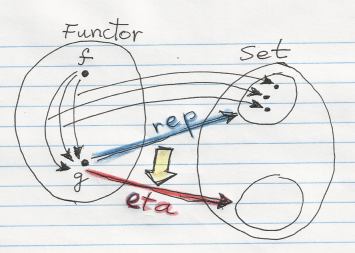
Now that we’ve got used to viewing functors as containers, let’s figure out what natural transformations are. A natural transformation is a mapping of functors that preserves their functorial nature. If functor F maps object A to X and another functor G maps A to Y, then a natural transformation from F to G must map X to Y. A mapping from X to Y is a morphism. So you can look at a natural transformation as a family of morphisms parameterized by A.

In Haskell, we turn all these objects A, X, and Y into types. We have two functors f and g acting on type a. A natural transformation will be a polymorphic function that maps f a to g a for any a.

forall a . f a -> g a

What does it mean in terms of containers? Very simple: A natural transformation is a way of re-packaging containers. It tells you how to take elements from one container and put them into another. It must do it without ever inspecting the elements themselves (it can, however, drop some elements or clone them).

Examples of natural transformations abound, but my favorite is safeHead. It takes the head element from a list container and repackages it into a Maybe container:

safeHead :: forall a . [a] -> Maybe a
safeHead []     = Nothing
safeHead (x:xs) = Just x

What about a more ambitions example: Let’s take a reader functor, Int -> a, and map it into the list functor [a]. The former corresponds to a container of a keyed by an integer, so it’s easily repackaged into a finite or an infinite list, for instance:

genInfList :: forall a . (Int -> a) -> [a]
genInfList f = fmap f [0..]

I’ll show you soon that all natural transformations from (Int -> a) to [a] have this form, and differ only by the choice of the list of integers (here, I arbitrarily picked [0..]).

A natural transformation, being a mapping of functors, must interact nicely with morphisms as well. The corresponding naturality condition translates easily into our container language. It tells you that it shouldn’t matter whether you first apply a function to the contents of a container (fmap over it) and then repackage it, or first repackage and then apply the function. This meshes very well with our intuition that repackaging doesn’t touch the elements of the container — it doesn’t breaks the eggs in the crate.

The Yoneda Lemma

Now let’s get back to the function application functor (the Reader functor). I said it had something to do with the Yoneda lemma. I wrote a whole blog about the Yoneda lemma, so I’m not going to repeat it here — just translate it into the container language.

What Yoneda says is that the reader is a universal container from which stuff can be repackaged into any other container. I just showed you how to repackage the Int reader into a list using fmap and a list of Int. It turns out that you can do the same for any type of reader and an arbitrary container type. You just provide a container full of “environments” and fmap the reader function over it. In my example, the environment type was Int and the container was a list.

Moreover, Yoneda says that there is a one-to-one correspondence between “repackaging schemes” and containers of environments. Given a container of environments you do the repackaging by fmapping the reader over it, as I did in the example. The inverse is also easy: given a repackaging, call it with an identity reader:

idReader :: Reader e e
idReader = Reader id

and you’ll get a container filled with environments.

Let me re-word it in terms of functors and natural transformations. For any functor f and any type e, all natural transformations of the form:

forall a . ((e -> a) -> f a)

are in one-to-one correspondence with values of the type f e. This is a pretty powerful equivalence. On the one hand you have a polymorphic function, on the other hand a polymorphic data structure, and they encode the same data. Except that things you do with functions are different than things you do with data structures so, depending on the context, one may be more convenient than the other.

For instance, if we apply the Yoneda lemma to the reader functor itself, we find out that all repackagings (natural transformations) between readers can be parameterized by functions between their environment types:

forall a . ((e -> a) -> (e' -> a)) ~ e' -> e

Or, you can look at this result as the CPS transform: Any function can be encoded in the Continuation Passing Style. The argument (e -> a) is the continuation. The forall quantifier tells us that the return type of the continuation is up to the caller. The caller might, for instance, decide to print the result, in which case they would call the function with the continuation that returns IO (). Or they might call it with id, which is itself polymorphic: a -> a.

Where Do Containers Come From?

A functor is a type constructor — it operates on types — but in a program you want to deal with data. A particular functor might define its data constructor: List and Maybe have constructors. A function, which we need in order to create an instance of the reader functor, may either be defined globally or through a lambda expression. You can’t construct an IO object, but there are some built-in runtime functions, like getChar or putChar that return IO.

If you have functions that produce containers you may compose them to create more complex containers, as in:

-- m is the functor
f :: a -> m b
g :: b -> m c
fmap g (f x) :: m (m c)

But the general ability to construct containers from scratch and to combine them requires special powers that are granted by successively more powerful classes of containers.

Pointed

The first special power is the ability to create a default container from an element of any type. The function that does that is called pure in the context of applicative and return in the context of a monad. To confuse things a bit more, there is a type class Pointed that defines just this ability, giving it yet another name, point:

class Functor f => Pointed f where
        point :: a -> f a

point is a natural transformation. You might object that there is no functor on the left hand side of the arrow, but just imagine seeing Identity there. Naturality just means that you can sneak a function under the functor using fmap:

fmap g (point x) = point (g x)

The presence of point means that there is a default, “trivial,” shape for the container in question. We usually don’t want this container to be empty (although it may — I’m grateful to Edward Kmett for correcting me on this point). It doesn’t mean that it’s a singleton, though — for ZipList, for instance, pure generates an infinite list of a.

Applicative

Once you have a container of one type, fmap lets you generate a container of another type. But since the function you pass to fmap takes only one argument, you can’t create more complex types that take more than one argument in their constructor. You can’t even create a container of (non-diagonal) pairs. For that you need a more general ability: to apply a multi-argument function to multiple containers at once.

Of course, you can curry a multi-argument function and fmap it over the first container, but the result will be a container of hungry functions waiting for more arguments.

h :: a -> b -> c
fmap h (m a) :: m (b -> c)

(Here, m stands for the functor, applicative, or the monad in question.)

What you need is the ability to apply a container of functions to a container of arguments. The function that does that is called <*> in the context of applicative, and ap in the context of monad.

(<*>) :: m (a -> b) -> m a -> m b

As I mentioned before, Applicative is also Pointed, with point renamed to pure. This lets you wrap any additional arguments to your multi-argument functions.

The intuition is that applicative brings to the table its ability to increase the complexity of objects stored in containers. A functor lets you modify the objects but it’s a one-input one-output transformation. An applicative can combine multiple sources of information. You will often see applicative used with data constructors (which are just functions) to create containers of object from containers of arguments. When the containers also carry state, as you’ll see when we talk about State, an applicative will also be able to reflect the state of the arguments in the state of the result.

Monad

The monad has the special power of collapsing containers. The function that does it is called join and it turns a container of containers into a single container:

join :: m (m a) -> m a

Although it’s not obvious at first sight, join is also a natural transformation. The fmap for the m . m functor is the square of the original fmap, so the naturality condition looks like this:

 fmap f . join = join . (fmap . fmap) f 

Every monad is also an applicative with return playing the role of pure and ap implementing <*>:

ap :: m (a -> b) -> m a -> m b
ap mf ma = join $ fmap (\f -> fmap f ma) mf

When working with the container interpretation, I find this view of a monad as an applicative functor with join more intuitive. In practice, however, it’s more convenient to define the monad in terms of bind, which combines application of a function a la fmap with the collapsing of the container. This is done using the function >>=:

(>>=) :: m a -> (a -> m b) -> m b
ma >>= k = join (fmap k ma)

Here, k is a function that produces containers. It is applied to a container of a, ma, using fmap. We’ve seen this before, but we had no way to collapse the resulting container of containers — join makes this possible.

Imagine a hierarchy of containment. You start with functions that produce containers. They “lift” your data to the level of containers. These are functions like putChar, data constructors like Just, etc. Then you have the “trivial” lifters of data called pure or return. You may operate on the data stored in containers by “lifting” a regular function using fmap. Applicative lets you lift multi-parameter functions to create containers of more complex data. You may also lift functions that produce containers to climb the rungs of containment: you get containers of containers, and so on. But only the monad provides the ability to collapse this hierarchy.

State

Let’s have a look at the state functor, the basis of the state monad. It’s very similar to the reader functor, except that it also modifies the environment. We’ll call this modifiable environment “state.” The modified state is paired with the return value of the function that defines the state functor:

newtype State s a = State (s -> (a, s))

As a container, the reader functor generalized the key/value store. How should we interpret the state functor in the container language? Part of it is still the key/value mapping, but we have the additional key/key mapping that describes the state transformation. (The state plays the role of the key.) Notice also that the action of fmap modifies the values, but doesn’t change the key mappings.

instance Functor (State s) where
  fmap f (State g) = State (\st -> let (x, st') = g st 
                                   in (f x, st'))

This is even more obvious if we separate the two mappings. Here’s the equivalent definition of the state functor in terms of two functions:

data State' s a = State' (s -> a) (s -> s)

The first function maps state to value: that’s our key/value store, identical to that of the reader functor. The second function is the state transition matrix. Their actions are quite independent:

runState' (State' f tr) s = (f s, tr s)

In this representation, you can clearly see that fmap only acts on the key/value part of the container, and its action on data is identical to that of the reader functor:

instance Functor (State' s) where
  fmap f (State' g tr) = State' (f . g) tr

In the container language, we like to separate the contents from the shape of the container. Clearly, in the case of the state functor, the transition matrix, not being influenced by fmap, is part of the shape.

A look at the Applicative instance for this representation of the state functor is also interesting:

instance Applicative (State' s) where
  pure x = State' (const x) id
  State' fg tr1 <*> State' fx tr2 =
      State' ff (tr2 . tr1)
    where
      ff st = let g = fg st
                  x = fx (tr1 st)
              in g x

The default container created by pure uses identity as its transition matrix. As expected, the action of <*> creates a new “shape” for the container, but it does it in a very regular way by composing the transition matrices. In the language of linear algebra, the transformation of state by the applicative functor would be called “linear.” This will not be true with monads.

You can also see the propagation of side effects: the values for the first and second argument are retrieved using different keys: The key for the retrieval of the function g is the original state, st; but the argument to the function, x, is retrieved using the state transformed by the transition matrix of the first argument (tr1 st). Notice however that the selection of keys is not influenced by the values stored in the containers.

But here’s the monad instance:

instance Monad (State' s) where
  return x = State' (const x) id
  State' fx tr >>= k =
      State' ff ttr
    where
      ff st  = let x = fx st
                   st' = tr st
                   State' fy tr' = k x
               in fy st' 
      ttr st = let x = fx st
                   st' = tr st
                   State' fy tr' = k x
               in tr' st'

What’s interesting here is that the calculation of the transition matrix requires the evaluation of the function k with the argument x. It means that the state transition is no longer linear — the decision which state to chose next may depend on the contents of the container. This is also visible in the implementation of join for this monad:

join :: State' s (State' s a) -> State' s a
join (State' ff ttr) = State' f' tr'
  where
    f' st  = let State' f tr = ff st
                 st'         = ttr st
             in f st'
    tr' st = let State' f tr = ff st
                 st'         = ttr st
             in tr st'

Here, the outer container stores the inner container as data. Part of the inner container is its transition matrix. So the decision of which transition matrix tr to use is intertwined with data in a non-linear way.

This non-linearity means that a monad is strictly more powerful than applicative, but it also makes composing monads together harder.

Conclusions

The only way to really understand a complex concept is to see it from as many different angles as possible. Looking at functors as containers provides a different perspective and brings new insights. For me it was the realization that functions can be seen as non-enumerable containers of values, and that the state monad can be seen as a key/value store with an accompanying state transition matrix that brought the aha! moments. It was also nice to explicitly see the linearity in the applicative’s propagation of state. It was surprising to discover the simplicity of the Yoneda lemma and natural transformations in the language of containers.

Bibliography and Acknowledgments

A container is not a very well defined term — an ambiguity I exploited in this blog post — but there is a well defined notion of finitary containers, and they indeed have a strong connection to functors. Russell O’Connor and Mauro Jaskelioff have recently shown that every traversable functor is a finitary container (I’m grateful to the authors for providing me with the preliminary copy of their paper, in which they have also independently and much more rigorously shown the connection between the Yoneda lemma for the functor category and the van Laarhoven formulation of the lens).


The WordPress.com stats helper monkeys prepared a 2013 annual report for this blog.

Here’s an excerpt:

The Louvre Museum has 8.5 million visitors per year. This blog was viewed about 220,000 times in 2013. If it were an exhibit at the Louvre Museum, it would take about 9 days for that many people to see it.

Click here to see the complete report.


There is an engineer and a mathematician in each of us. My blog posts, for instance, alternate between discussing write ordering in the x86 processor, and explaining abstract ideas from category theory. I might be a bit extreme in this respect, but even in everyday programming we often switch between the focused, low-level, practical thinking of an engineer and the holistic, global, abstract thinking of a mathematician. Sometimes we write a for loop; sometimes we holistically apply std::transform to a vector. Sometimes we write imperative step-by-step programs; and sometimes we write declarative ones, letting the compiler figure out the steps.

What I find fascinating is that these two approaches also manifest themselves in mathematics. There are constructive proofs that resemble the work of an engineer; and there are proofs of existence, that resemble the work of a philosopher. An entity may be defined by showing how to construct it, or it might be defined by its universal property — by being the most general or the most specific among its peers. A universal description is favored by category theorists, especially if it reduces their dependency on Set Theory. It’s not that category theorists hate set theory, but they definitely like to limit their reliance on it.

In this post I’ll show you the two ways of defining a free monoid. If the term monoid is not familiar to you, don’t despair; it’s a very simple construct, and you’ve seen it and used it many times. The classic example of a monoid is the set of strings with string concatenation. Another is the set of natural numbers with addition (or multiplication — either will work).

Free Monoid

A monoid is a set with a binary operation — let’s just call it multiplication and denote it by the infix * (you’ll also see it called, in Haskell, mappend, ++, <>…). This binary operation must obey certain laws. The first law is that there is a special element called unit, e, with the property that for any a:

a * e = e * a = a

(You’ll also see it called mempty.) The second law is that of associativity:

a * (b * c) = (a * b) * c

There are many examples of monoids, but there is a special class of them called free monoids. The easiest way to understand what a free monoid is, is to construct one. Just pick a set, any set, and call it the set of generators. Then define multiplication in the laziest, dumbest possible way. First, add one more element to the set and call it a unit. Define multiplication by unit to always return the other multiplicand. Then, for every pair of generators create a new element and call it their product. Define products of products the same way — every time you need to multiply two existing elements, create a new one, call it their product, and add it to the growing set. The only tricky part is to make sure that thusly defined product is associative. So for every triple of elements, a, b, and c, you have to identify a * (b * c) with (a * b) * c.

Here’s a little mnemonic trick that may help you keeping track of associativity. Assign letters of the alphabet to your generators. Say, you have less than 26 generators and you call them a, b, c, etc. Reserve letter z for your unit element. When asked for the product of, say, a and t, call it at. The product of c and at will be cat, and so on. This way, you’ll automatically call the product of ca with t, cat, as you should.

As you can see a free monoid generated by an alphabet is equivalent to the set of strings, with product defined as string concatenation.

What happens when your original set has just one element, say a? The free monoid based on this set would contain the unit z and all the powers of a of the form aaa.... Writing long strings of as is boring, so instead let’s just length-encode them: a as 1, aa as 2, and so on. It’s natural to assign zero to z. We have just reinvented natural numbers with “product” being the addition.

Lists are free monoids too. Take any finite or infinite set and create ordered lists of its elements. Your unit element is the empty list, and “multiplication” is the concatenation of lists. Strings are just a special type of lists based on a finite set of generators. But you can have lists of integers, 3-D points, or even lists of lists.

Not all monoids are free, though. Take for instance addition modulo 4. You start with four elements: 0, 1, 2, and 3. But the sum of 2 and 3 is 1 (5 mod 4). Were it a free monoid, 2+3 would be a totally new element, but here we identified it with the existing element 1.

The question is, can we obtain any monoid by identifying some elements of the corresponding free monoid? The modulo 4 monoid, for instance, could be obtained by identifying all natural numbers that have the same remainder when divided by 4.

The answer is yes, and it’s an example of a very important notion in category theory called universality. A free monoid is universal. Here’s what it means: I have a set of generators and a free monoid built from it. Give me any monoid and select any elements in it to correspond to the generators of my free monoid. I can show you a unique mapping m of my free monoid to your monoid that not only maps my generators to your selected elements, but also preserves multiplication. In other words, if a * b = c in my monoid, then m(a) * m(b) = m(c) in your monoid.

Notice that the mapping might not cover the whole target monoid. It might cover a sub-monoid. But within that sub-monoid, for each element in my monoid there will be a corresponding element in yours. In general, multiple elements in my monoid may be mapped to a single element in yours. This way your monoid has the same structure as mine, except that some elements have been identified.

Any monoid can be obtained from a free monoid by identifying some elements.

Categorical Monoid

You might find the above theorem in a category theory text (see, for instance, Saunders Mac Lane, Categories for the Working Mathematician, Corollary 2 on p. 50) and not recognize it. That’s because category theoreticians don’t like treating monoids as sets of elements. They prefer to see a monoid as a shapeless object whose properties are encoded in morphisms — arrows from a monoid to itself.

How do we reconcile these two views of monoids? On the one hand you have a set of elements with multiplication, on the other hand a monolithic blob with arrows.

Here’s one way: Consider what happens when you pick one element of a monoid and apply it to all elements — say, by left multiplication. You get a function acting on this set (in Haskell we call this function an operator section). That’s your morphism. Notice that you can compose such morphisms just like you compose functions: left multiplication by “a” composed with left multiplication by “b” is the same function as left multiplication by “a * b”. The set of these morphisms/functions — one for each element — together with the usual function composition — tells you everything about the monoid. It gives you the categorical description of it: A monoid is a category with a single object (“mono” means one, single) and a bunch of morphisms acting on it.

There is also a bigger Category of Monoids, where monoids are the objects and morphisms map monoids into monoids preserving their structure (they map products into products). Some of these monoids are free, others are not.

We know how to construct a free monoid starting from a set of generators, but how can we tell which of the abstract blobs with morphisms is free and which isn’t? And how do we even begin talking about generators if we vowed not to view monoids as sets?

Universal Construction

We have to work our way back from abstract monoids to sets. But to do that we need a functor because we’re going between categories. Our source is the category of monoids, and our target is the category of sets, where objects are sets and morphisms are regular functions.

Just a reminder: A functor is a mapping between categories. It maps objects into objects and morphisms into morphisms; but not willy-nilly — it has to preserve composition. So if one morphism is a composition of two others, it’s image under the functor must also be the composition of the two images.

In our case we will be mapping the category of monoids into the category of sets. But once you mapped a monoid into a set (its, so called, underlying set), you have forgotten its structure. You have forgotten that some functions were “special” because they corresponded to the morphisms of the original monoid. All functions are now equal. This kind of functor that forgets structure is aptly called a forgetful functor.

Our goal is to describe a free monoid corresponding to a set of generators X. X is just a regular set, nothing fancy, but we can’t look for it inside a monoid because a monoid is not a set any more. Fortunately we have our forgetful functor U, which maps monoids into sets. So instead of looking for generators inside monoids (which we can’t do), we’ll look for them inside those underlying sets. Given a monoid M, we just pick a function p: X -> U M. The image of X under p will serve as candidate generators.

Now let’s take another monoid L and do the same thing. We map our generators into the set U L (the set obtained from L using the same forgetful functor U). Call this mapping h: X -> U L. Now, U is a functor, so it maps monoids to sets and monoid morphisms to functions. So if there is a morphism m from M to L, there is a corresponding function from U M to U L (we’ll call this function U m). This is just a function mapping the set that’s underlying one monoid into the set that’s underlying another monoid.

The first set, U M, contains the images of our generators under p. Our function U m will map those candidate generators into some set in U L. Now, U L also contains candidate generators — the images of X under h. What are the chances that those two sets are the same? Slim but not zero! If we can pick m so that they overlap, we will have come as close as possible to the idea of the two monoids “sharing the same generators.” (See the following illustration.)

Universal construction of a free monoid generated by X

Universal construction of a free monoid generated by X

So given two monoids M and L and a set of generators X we can create candidate sets of generators in U M and U L. If we’re lucky, we can find a monoid morphism m that maps M to L and whose projection using U maps one candidate set of generators into the other.

Now zoom out to the category of monoids and draw an arrow between any M and L whenever such m exists. What you’ll find out, to your great amazement, is that there is one unique monoid (up to an isomorphism) that has all arrows going out and none coming in. This universal monoid is the free monoid constructed from the set of generators X. The two completely different descriptions converge!

Conclusion

How does it work? What’s the intuition behind it?

A lot of mathematicians secretly (or not so secretly) subscribe to Plato’s philosophy. A monoid is a Platonic object that can’t be observed directly, but which can cast a shadow on the wall of the cave we live in. This shadow is the underlying set: the result of a forgetful functor. The morphisms between monoids preserve their nature; theirs shadows, though, are mere functions.

Functions may be invertible, but often they conflate elements together. So if you have a flow of functions from one set to a bunch of others, they will tend to smooth out the differences, collapse multiple elements into one. So if there is one shadow of a monoid that dominates all others that are sharing the same generators — and there always is one — it must be the shadow of the free one. It is the one that has the largest selection of distinct elements, since every multiplication produces a new element (mitigated only by the requirements of associativity and the need for the unit).

Appendix: A Bonus Free Object

Free monoid is an example of a larger class of free objects. Free object is a powerful notion in category theory that generalizes the idea of a basis. Instead of the category of monoids let’s take any category that supports a faithful functor into the category of sets. A faithful functor is a functor that maps distinct morphism into distinct functions — it doesn’t mash them together. This will be our forgetful functor U. It maps an object A from our category to a set U A; and we can inject our basis X into this set, just like we did with generators. Object A is called universal if, for any other object B and any injection of X into U B, there is a unique morphism from A to B that “preserves” the basis. Again, by preserving the basis we mean that the image of our morphism under U maps one injected basis into the other.


In my previous blog posts I described C++ implementations of two basic functional data structures: a persistent list and a persistent red-black tree. I made an argument that persistent data structures are good for concurrency because of their immutability. In this post I will explain in much more detail the role of immutability in concurrent programming and argue that functional data structures make immutability scalable and composable.

Concurrency in 5 Minutes

To understand the role of functional data structures in concurrent programming we first have to understand concurrent programming. Okay, so maybe one blog post is not enough, but I’ll try my best at mercilessly slashing through the complexities and intricacies of concurrency while brutally ignoring all the details and subtleties.

The archetype for all concurrency is message passing. Without some form of message passing you have no communication between processes, threads, tasks, or whatever your units of execution are. The two parts of “message passing” loosely correspond to data (message) and action (passing). So there is the fiddling with data by one thread, some kind of handover between threads, and then the fiddling with data by another thread. The handover process requires synchronization.

There are two fundamental problems with this picture: Fiddling without proper synchronization leads to data races, and too much synchronization leads to deadlocks.

Communicating Processes

Let’s start with a simpler world and assume that our concurrent participants share no memory — in that case they are called processes. And indeed it might be physically impossible to share memory between isolated units because of distances or hardware protection. In that case messages are just pieces of data that are magically transported between processes. You just put them (serialize, marshall) in a special buffer and tell the system to transmit them to someone else, who then picks them up from the system.

So the problem reduces to the proper synchronization protocols. The theory behind such systems is the good old CSP (Communicating Sequential Processes) from the 1970s. It has subsequently been extended to the Actor Model and has been very successful in Erlang. There are no data races in Erlang because of the isolation of processes, and no traditional deadlocks because there are no locks (although you can have distributed deadlocks when processes are blocked on receiving messages from each other).

The fact that Erlang’s concurrency is process-based doesn’t mean that it’s heavy-weight. The Erlang runtime is quite able to spawn thousands of light-weight user-level processes that, at the implementation level, may share the same address space. Isolation is enforced by the language rather than by the operating system. Banning direct sharing of memory is the key to Erlang’s success as the language for concurrent programming.

So why don’t we stop right there? Because shared memory is so much faster. It’s not a big deal if your messages are integers, but imagine passing a video buffer from one process to another. If you share the same address space (that is, you are passing data between threads rather than processes) why not just pass a pointer to it?

Shared Memory

Shared memory is like a canvas where threads collaborate in painting images, except that they stand on the opposite sides of the canvas and use guns rather than brushes. The only way they can avoid killing each other is if they shout “duck!” before opening fire. This is why I like to think of shared-memory concurrency as the extension of message passing. Even though the “message” is not physically moved, the right to access it must be passed between threads. The message itself can be of arbitrary complexity: it could be a single word of memory or a hash table with thousands of entries.

It’s very important to realize that this transfer of access rights is necessary at every level, starting with a simple write into a single memory location. The writing thread has to send a message “I have written” and the reading thread has to acknowledge it: “I have read.” In standard portable C++ this message exchange might look something like this:

std::atomic x = false;
// thread one
x.store(true, std::memory_order_release);
// thread two
x.load(std::memory_order_acquire);

You rarely have to deal with such low level code because it’s abstracted into higher order libraries. You would, for instance, use locks for transferring access. A thread that acquires a lock gains unique access to a data structure that’s protected by it. It can freely modify it knowing that nobody else can see it. It’s the release of the lock variable that makes all those modifications visible to other threads. This release (e.g., mutex::unlock) is then matched with the subsequent acquire (e.g., mutex::lock) by another thread. In reality, the locking protocol is more complicated, but it is at its core based on the same principle as message passing, with unlock corresponding to a message send (or, more general, a broadcast), and lock to a message receive.

The point is, there is no sharing of memory without communication.

Immutable Data

The first rule of synchronization is:

The only time you don’t need synchronization is when the shared data is immutable.

We would like to use as much immutability in implementing concurrency as possible. It’s not only because code that doesn’t require synchronization is faster, but it’s also easier to write, maintain, and reason about. The only problem is that:

No object is born immutable.

Immutable objects never change, but all data, immutable or not, must be initialized before being read. And initialization means mutation. Static global data is initialized before entering main, so we don’t have to worry about it, but everything else goes through a construction phase.

First, we have to answer the question: At what point after initialization is data considered immutable?

Here’s what needs to happen: A thread has to somehow construct the data that it destined to be immutable. Depending on the structure of that data, this could be a very simple or a very complex process. Then the state of that data has to be frozen — no more changes are allowed. But still, before the data can be read by another thread, a synchronization event has to take place. Otherwise the other thread might see partially constructed data. This problem has been extensively discussed in articles about the singleton pattern, so I won’t go into more detail here.

One such synchronization event is the creation of the receiving thread. All data that had been frozen before the new thread was created is seen as immutable by that thread. That’s why it’s okay to pass immutable data as an argument to a thread function.

Another such event is message passing. It is always safe to pass a pointer to immutable data to another thread. The handover always involves the release/acquire protocol (as illustrated in the example above).

All memory writes that happened in the first thread before it released the message become visible to the acquiring thread after it received it.

The act of message passing establishes the “happens-before” relationship for all memory writes prior to it, and all memory reads after it. Again, these low-level details are rarely visible to the programmer, since they are hidden in libraries (channels, mailboxes, message queues, etc.). I’m pointing them out only because there is no protection in the language against the user inadvertently taking affairs into their own hands and messing things up. So creating an immutable object and passing a pointer to it to another thread through whatever message passing mechanism is safe. I also like to think of thread creation as a message passing event — the payload being the arguments to the thread function.

The beauty of this protocol is that, once the handover is done, the second (and the third, and the fourth, and so on…) thread can read the whole immutable data structure over and over again without any need for synchronization. The same is not true for shared mutable data structures! For such structures every read has to be synchronized at a non-trivial performance cost.

However, it can’t be stressed enough that this is just a protocol and any deviation from it may be fatal. There is no language mechanism in C++ that may enforce this protocol.

Clusters

As I argued before, access rights to shared memory have to be tightly controlled. The problem is that shared memory is not partitioned nicely into separate areas, each with its own army, police, and border controls. Even though we understand that an object is frozen after construction and ready to be examined by other threads without synchronization, we have to ask ourselves the question: Where exactly does this object begin and end in memory? And how do we know that nobody else claims writing privileges to any of its parts? After all, in C++ it’s pointers all the way. This is one of the biggest problems faced by imperative programmers trying to harness concurrency — who’s pointing where?

For instance, what does it mean to get access to an immutable linked list? Obviously, it’s not enough that the head of the list never changes, every single element of the list must be immutable as well. In fact, any memory that can be transitively accessed from the head of the list must be immutable. Only then can you safely forgo synchronization when accessing the list, as you would in a single-threaded program. This transitive closure of memory accessible starting from a given pointer is often called a cluster. So when you’re constructing an immutable object, you have to be able to freeze the whole cluster before you can pass it to other threads.

But that’s not all! You must also guarantee that there are no mutable pointers outside of the cluster pointing to any part of it. Such pointers could be inadvertently used to modify the data other threads believe to be immutable.

That means the construction of an immutable object is a very delicate operation. You not only have to make sure you don’t leak any pointers, but you have to inspect every component you use in building your object for potential leaks — you either have to trust all your subcontractors or inspect their code under the microscope. This clearly is no way to build software! We need something that it scalable and composable. Enter…

Functional Data Structures

Functional data structures let you construct new immutable objects by composing existing immutable objects.

Remember, an immutable object is a complete cluster with no pointers sticking out of it, and no mutable pointers poking into it. A sum of such objects is still an immutable cluster. As long as the constructor of a functional data structure doesn’t violate the immutability of its arguments and does not leak mutable pointers to the memory it is allocating itself, the result will be another immutable object.

Of course, it would be nice if immutability were enforced by the type system, as it is in the D language. In C++ we have to replace the type system with discipline, but still, it helps to know exactly what the terms of the immutability contract are. For instance, make sure you pass only (const) references to other immutable objects to the constructor of an immutable object.

Let’s now review the example of the persistent binary tree from my previous post to see how it follows the principles I described above. In particular, let me show you that every Tree forms an immutable cluster, as long as user data is stored in it by value (or is likewise immutable).

The proof proceeds through structural induction, but it’s easy to understand. An empty tree forms an immutable cluster trivially. A non-empty tree is created by combining two other trees. We can assume by the inductive step that both of them form immutable clusters:

Tree(Tree const & lft, T val, Tree const & rgt)

In particular, there are no external mutating pointers to lft, rgt, or to any of their nodes.

Inside the constructor we allocate a fresh node and pass it the three arguments:

Tree(Tree const & lft, T val, Tree const & rgt)
      : _root(std::make_shared<const Node>(lft._root, val, rgt._root))
{}

Here _root is a private member of the Tree:

std::shared_ptr<const Node> _root;

and Node is a private struct defined inside Tree:

struct Node
{
   Node(std::shared_ptr<const Node> const & lft
       , T val
       , std::shared_ptr<const Node> const & rgt)
   : _lft(lft), _val(val), _rgt(rgt)
   {}

   std::shared_ptr<const Node> _lft;
   T _val;
   std::shared_ptr<const Node> _rgt;
};

Notice that the only reference to the newly allocated Node is stored in _root through a const pointer and is never leaked. Moreover, there are no methods of the tree that either modify or expose any part of the tree to modification. Therefore the newly constructed Tree forms an immutable cluster. (With the usual caveat that you don’t try to bypass the C++ type system or use other dirty tricks).

As I discussed before, there is some bookkeeping related to reference counting in C++, which is however totally transparent to the user of functional data structures.

Conclusion

Immutable data structures play an important role in concurrency but there’s more to them that meets the eye. In this post I tried to demonstrate how to use them safely and productively. In particular, functional data structures provide a scalable and composable framework for working with immutable objects.

Of course not all problems of concurrency can be solved with immutability and not all immutable object can be easily created from other immutable objects. The classic example is a doubly-linked list: you can’t add a new element to it without modifying pointers in it. But there is a surprising variety of composable immutable data structures that can be used in C++ without breaking the rules. I will continue describing them in my future blog posts.


Persistent trees are more interesting than persistent lists, which were the topic of my previous blog. In this installment I will concentrate on binary search trees. Such trees store values that can be compared to each other (they support total ordering). Such trees may be used to implement sets, multisets, or associated arrays. Here I will focus on the simplest of those, the set — the others are an easy extensions of the same scheme.

A set must support insertion, and membership test (I’ll leave deletion as an exercise). These operations should be doable, on average, in logarithmic time, O(log(N)). Only balanced trees, however, can guarantee logarithmic time even in the worst case. A simple tree may sometimes degenerate to a singly-linked list, with performance dropping to O(N). I will start with a simple persistent tree and then proceed with a balanced red-black tree.

Persistent Binary Search Tree

As with lists, we will start with an abstract definition:

A tree is either empty or contains a left tree, a value, and a right tree.

This definition translates into a data structure with two constructors:

template<class T>
class Tree {
public:
    Tree(); // empty tree
    Tree(Tree const & lft, T val, Tree const & rgt)
};

Just as we did with persistent lists, we’ll encode the empty/non-empty tree using null/non-null (shared) pointer to a node. A Node represents a non-empty tree:

   struct Node
   {
       Node(std::shared_ptr<const Node> const & lft
          , T val
          , std::shared_ptr<const Node> const & rgt)
       : _lft(lft), _val(val), _rgt(rgt)
       {}

       std::shared_ptr<const Node> _lft;
       T _val;
       std::shared_ptr<const Node> _rgt;
   };

Here’s the complete construction/deconstruction part of the tree. Notice how similar it is to the list from my previous post. All these methods are const O(1) time, as expected. As before, the trick is to construct a new object (Tree) from big immutable chunks (lft and rgt), which can be safely put inside shared pointers without the need for deep copying.

template<class T>
class Tree
{
    struct Node;
    explicit Tree(std::shared_ptr<const Node> const & node) 
    : _root(node) {} 
public:
    Tree() {}
    Tree(Tree const & lft, T val, Tree const & rgt)
      : _root(std::make_shared<const Node>(lft._root, val, rgt._root))
    {
        assert(lft.isEmpty() || lft.root() < val);
        assert(rgt.isEmpty() || val < rgt.root());       
    }
    bool isEmpty() const { return !_root; }
    T root() const {
        assert(!isEmpty());
        return _root->_val;
    }
    Tree left() const {
        assert(!isEmpty());
        return Tree(_root->_lft);
    }
    Tree right() const {
        assert(!isEmpty());
        return Tree(_root->_rgt);
    }
private:
    std::shared_ptr<const Node> _root;
};

Insert

The persistent nature of the tree manifests itself in the implementation of insert. Instead of modifying the existing tree, insert creates a new tree with the new element inserted in the right place. The implementation is recursive, so imagine that you are at a subtree of a larger tree. This subtree might be empty. Inserting an element into an empty tree means creating a single-node tree with the value being inserted, x, and two empty children.

On the other hand, if you’re not in an empty tree, you can retrieve the root value y and compare it with x. If x is less then y, it has to be inserted into the left child. If it’s greater, it must go into the right child. In both cases we make recursive calls to insert. If x is neither less nor greater than y, we assume it’s equal (that’s why we need total order) and ignore it. Remember, we are implementing a set, which does not store duplicates.

Tree insert(T x) const {
    if (isEmpty())
        return Tree(Tree(), x, Tree());
    T y = root();
    if (x < y)
        return Tree(left().insert(x), y, right());
    else if (y < x)
        return Tree(left(), y, right().insert(x));
    else
        return *this; // no duplicates
}

Now consider how many new nodes are created during an insertion. A new node is only created in the constructor of a tree (in the code: std::make_shared<const Node>(lft._root, val, rgt._root)). The left and right children are not copied, they are stored by reference. At every level of insert, a tree constructor is called at most once. So in the worst case, when we recurse all the way to the leaves of the tree, we only create h nodes, where h is the height of the tree. If the tree is not too much out of balance its height scales like a logarithm of the number of nodes. To give you some perspective, if you store a billion values in a tree, an insertion will cost you 30 copies on average. If you need a logarithmic bound on the worst case, you’d have to use balanced trees (see later).

If you study the algorithm more closely, you’ll notice that only the nodes that are on the path from the root to the point of insertion are modified.

Testing for membership in a persistent tree is no different than in a non-persistent one. Here’s the recursive algorithm:

bool member(T x) const {
    if (isEmpty())
        return false;
    T y = root();
    if (x < y)
        return left().member(x);
    else if (y < x)
        return right().member(x);
    else
        return true;
}

When using C++11, you might take advantage of the initializer list constructor to initialize a tree in one big swoop like this:

Tree t{ 50, 40, 30, 10, 20, 30, 100, 0, 45, 55, 25, 15 };

.

Here’s the implementation of such constructor, which works in O(N*log(N)) average time (notice that it effectively sorts the elements, and O(N*log(N)) is the expected asymptotic behavior for sort):

Tree(std::initializer_list<T> init) {
    Tree t;
    for (T v: init) {
        t = t.insert(v);
    }
    _root = t._root;
}

Persistent Red-Black Tree

If you want to keep your tree reasonably balanced — that is guarantee that its height is on the order of log(N) — you must do some rebalancing after inserts (or deletes). Care has to be taken to make sure that rebalancing doesn’t change the logarithmic behavior of those operations. The balance is often expressed using some invariants. You can’t just require that every path from root to leaf be of equal length, because that would constrain the number of elements to be always a power of two. So you must give it some slack.

In the case of a red-black tree, the invariants are formulated in terms of colors. Every node in the tree is marked as either red or black. These are the two invariants that have to be preserved by every operation:

  1. Red invariant: No red node can have a red child
  2. Black invariant: Every path from root to an empty leaf node must contain the same number of black nodes — the black height of the tree.

This way, if the shortest path in a tree is all black, the longest path could only be twice as long, containing one red node between each pair of black nodes. The height of such a tree could only vary between (all black) log(N) and (maximum red) 2*log(N).

With these constraints in mind, the re-balancing can be done in log(N) time by localizing the modifications to the nearest vicinity of the path from the root to the point of insertion or deletion.

Let’s start with basic definitions. The node of the tree will now store its color:

enum Color { R, B };

Otherwise, it’s the same as before:

    struct Node
    {
        Node(Color c, 
            std::shared_ptr const & lft, 
            T val, 
            std::shared_ptr const & rgt)
            : _c(c), _lft(lft), _val(val), _rgt(rgt)
        {}
        Color _c;
        std::shared_ptr _lft;
        T _val;
        std::shared_ptr _rgt;
    };

An empty tree will be considered black by convention.

The membership test ignores colors so we don’t have to re-implement it. In fact the search performance of a persistent RB Tree is exactly the same as that of an imperative RB Tree. You pay no penalty for persistence in search.

With insertion, you pay the penalty of having to copy the path from root to the insertion point, which doesn’t change its O(log(N)) asymptotic behavior. As I explained before, what you get in exchange is immutability of every copy of your data structure.

The Balancing

Let’s have a look at the previous version of insert and figure out how to modify it so the result preserves the RB Tree invariants.

Tree insert(T x) const {
    if (isEmpty())
        return Tree(Tree(), x, Tree());
    T y = root();
    if (x < y)
        return Tree(left().insert(x), y, right());
    else if (y < x)
        return Tree(left(), y, right().insert(x));
    else
        return *this; // no duplicates
}

Let’s first consider the most difficult scenario: the insertion into a maximum capacity tree for a given black height. Such a tree has alternating levels of all black and all red nodes. The only way to increase its capacity is to increase its black height. The cheapest way to add one more black level to all paths (thus preserving the black invariant) is to do it at the root (for instance, lengthening all the path at the leaves would require O(N) red-to-black re-paintings).

So here’s the plan: We’ll insert a new node at the leaf level and make it red. This won’t break the black invariant, but may break the red invariant (if the parent node was red). We’ll then retrace our steps back to the root, percolating any red violation up. Then, at the top level, we’ll paint the resulting root black, thus killing two birds with one stone: If we ended up with a red violation at the top, this will fix it and, at the same time, increase the black height of the whole tree.

It’s important that during percolation we never break the black invariant.

So here’s how we execute this plan: insert will call the recursive insertion/re-balancing method ins, which might return a red-topped tree. We’ll paint that root black (if it’s already black, it won’t change anything) and return it to the caller:

RBTree insert(T x) const {
    RBTree t = ins(x);
    return RBTree(B, t.left(), t.root(), t.right());
}

In the implementation of ins, the first case deals with an empty tree. This situation happens when it’s the first insertion into an empty tree or when, during the recursive process, we’ve reached the insertion point at the bottom of the tree. We create a red node and return it to the caller:

if (isEmpty())
  return RBTree(R, RBTree(), x, RBTree());

Notice that, if this new node was inserted below another red node, we are creating a red violation. If that node was the root of the whole tree, insert will repaint it immediately. If it weren’t, and we pop one level up from recursion, we’ll see that violation. We can’t fix it at that point — for that we’ll have to pop one more level, up to the black parent, where we have more nodes to work with.

Here are the details of ins: We’ll follow the same logic as in the non-balanced tree, thus preserving the ordering of values; but instead of reconstructing the result tree on the spot we’ll call a function balance, which will do that for us in a semi-balanced way (that is, with a possibility of a red violation, but only at the very top).

RBTree ins(T x) const
{
    if (isEmpty())
        return RBTree(R, RBTree(), x, RBTree());
    T y = root();
    Color c = rootColor();
    if (x < y)
        return balance(c, left().ins(x), y, right());
    else if (y < x)
        return balance(c, left(), y, right().ins(x));
    else
        return *this; // no duplicates
}

Just like the constructor of the red-black tree, balance takes the following arguments: color, left subtree, value, and right subtree. Depending on the result of the comparison, the new element is inserted either into the left or the right subtree.

As I explained, balance, and consequently ins, cannot fix the red violation when they are sitting on it. All they can do is to make sure that the violation is at the very top of the tree they return. So when we call balance with the result of ins, as in:

balance(c, left().ins(x), y, right())

or:

balance(c, left(), y, right().ins(x))

the left or the right subtree, respectively, may be semi-balanced. This is fine because balance can then rotate this violation away.

So the interesting cases for balance are the ones that rebuild a black node with either the left or the right subtree having a red violation at the top.

There are four possible cases depending on the position of the violation. In each case we can rearrange the nodes in such a way that the violation disappears and the ordering is preserved. In the pictures below I have numbered the nodes and subtrees according to the order of the values stored in them. Remember that all values in the left subtree are less than the value stored in the node, which in turn is less than all the values in the right subtree.

Fig 1

Rotating lft.doubledLeft()

Fig 1

Rotating lft.doubledRight()()

Fig 1

Rotating rgt.doubledLeft()

Fig 1

Rotating rgt.doubledRight()()

Each rotation creates a tree that preserves both invariants. Notice, however, that the result of the rotation is always red-tipped, even though we were rebuilding a node that was originally black. So if the parent of that node was red, our caller will produce a red violation (it will call balance with red color as its argument, which will fall through to the default case). This violation will be then dealt with at the parent’s parent level.

static RBTree balance(Color c
                    , RBTree const & lft
                    , T x
                    , RBTree const & rgt)
{
   if (c == B && lft.doubledLeft())
        return RBTree(R
                    , lft.left().paint(B)
                    , lft.root()
                    , RBTree(B, lft.right(), x, rgt));
    else if (c == B && lft.doubledRight())
        return RBTree(R
                    , RBTree(B, lft.left(), lft.root(), lft.right().left())
                    , lft.right().root()
                    , RBTree(B, lft.right().right(), x, rgt));
    else if (c == B && rgt.doubledLeft())
        return RBTree(R
                    , RBTree(B, lft, x, rgt.left().left())
                    , rgt.left().root()
                    , RBTree(B, rgt.left().right(), rgt.root(), rgt.right()));
    else if (c == B && rgt.doubledRight())
        return RBTree(R
                    , RBTree(B, lft, x, rgt.left())
                    , rgt.root()
                    , rgt.right().paint(B));
    else
        return RBTree(c, lft, x, rgt);
}

For completeness, here are the auxiliary methods used in the implementation of balance:

bool doubledLeft() const {
    return !isEmpty()
        && rootColor() == R
        && !left().isEmpty()
        && left().rootColor() == R;
}
bool doubledRight() const {
    return !isEmpty()
        && rootColor() == R
        && !right().isEmpty()
        && right().rootColor() == R;
}
RBTree paint(Color c) const {
    assert(!isEmpty());
    return RBTree(c, left(), root(), right());
}

Conclusion

Our implementation of the persistent red-black tree follows the Chris Okasaki’s book. As Chris asserts, this is one of the fastest implementations there is, and he offers hints to make it even faster. Of course there are many imperative implementations of red-black trees, including STL’s std::set and std::map. Persistent RB-trees match their performance perfectly when it comes to searching. Insertion and deletion, which are O(log(N)) for either implementation, are slower by a constant factor because of the need to copy the path from root to leaf. On the other hand, the persistent implementation is thread-safe and synchronization-free (except for reference counting in shared_ptr — see discussion in my previous blog).

Complete code is available at GitHub.

Acknowledgment

I’d like to thank Eric Niebler for reading the draft and telling me which of my explanations were more abstruse than usual.

Haskell Code

For comparison, here’s the original Haskell code. You can see that the C++ implementation preserves its structure pretty well. With proper optimization tricks (unboxing and eager evaluation) the Haskell code should perform as well as its C++ translation.

Regular (unbalanced) binary search tree:

data Tree a = Empty | Node (Tree a) a (Tree a)

member x Empty = False
member x (Node lft y rgt) =
    if x < y then member x lft
    else if y < x then member x rgt
    else True

insert x Empty = Node Empty x Empty
insert x t@(Node lft y rgt) =
    if x < y then Node (insert x lft) y rgt
    else if y < x then Node lft y (insert x rgt)
    else t

Balanced Red-Black tree:

data Color = R | B

data Tree a = Empty | Node Color (Tree a) a (Tree a)

member x Empty = False
member x (Node _ lft y rgt) =
    if x < y then member x lft
    else if y < x then member x rgt
    else True

insert x tree = Node B left val right
  where
      ins Empty = Node R Empty x Empty
      ins t@(Node c lft y rgt) =
          if (x < y) then balance c (ins lft) y rgt
          else if (y < x) then balance c lft y (ins rgt)
          else t
      Node _ left val right = ins tree -- pattern match result of ins


balance B (Node R (Node R a x b) y c) z d = 
    Node R (Node B a x b) y (Node B c z d)
balance B (Node R a x (Node R b y c)) z d = 
    Node R (Node B a x b) y (Node B c z d)
balance B a x (Node R (Node R b y c) z d) = 
    Node R (Node B a x b) y (Node B c z d)
balance B a x (Node R b y (Node R c z d)) = 
    Node R (Node B a x b) y (Node B c z d)
balance color a x b = Node color a x b

“Data structures in functional languages are immutable.”

What?! How can you write programs if you can’t mutate data? To an imperative programmer this sounds like anathema. “Are you telling me that I can’t change a value stored in a vector, delete a node in a tree, or push an element on a stack?” Well, yes and no. It’s all a matter of interpretation. When you give me a list and I give you back the same list with one more element, have I modified it or have I constructed a brand new list with the same elements plus one more?

Why would you care? Actually, you might care if you are still holding on to your original list. Has that list changed? In a functional language, the original data structure will remain unmodified! The version from before the modification persists — hence such data structures are called persistent (it has nothing to do with being storable on disk).

In this post I will discuss the following aspects of persistent data structures:

  • They are immutable, therefore
    • They are easier to reason about and maintain
    • They are thread-safe
  • They can be implemented efficiently
  • They require some type of resource management to “garbage collect” them.

I will illustrate these aspects on a simple example of a persistent linked list implemented in C++.

Motivation

There is a wealth of persistent data structures in functional languages, a lot of them based on the seminal book by Chris Okasaki, Purely Functional Data Structures (based on his thesis, which is available online). Unfortunately, persistent data structures haven’t found their way into imperative programming yet. In this series of blog posts I’ll try to provide the motivation for using functional data structures in imperative languages and start translating some of them into C++. I believe that persistent data structures should be part of every C++ programmer’s toolbox, especially one interested in concurrency and parallelism.

Persistence and Immutability

What’s the advantage of persistent data structures? For one, they behave as if they were immutable, yet you can modify them. The trick is that the modifications never spread to the aliases of the data structure — nobody else can observe them other that the mutator itself. This way you avoid any implicit long-distance couplings. This is important for program maintenance — you know that your bug fixes and feature tweaks will remain localized, and you don’t have to worry about breaking remote parts of the program that happen to have access to the same data structure.

There is another crucial advantage of immutable data structures — they are thread safe! You can’t have a data race on a structure that is read-only. Since copies of a persistent data structure are immutable, you don’t need to synchronize access to them. (This is, by the way, why concurrent programming is much easier in functional languages.)

Persistence and Multithreading

So if you want just one reason to use persistent data structures — it’s multithreading. A lot of conventional wisdom about performance is void in the face of multithreading. Concurrent and parallel programming introduces new performance criteria. It forces you to balance the cost of accessing data structures against the cost of synchronization.

Synchronization is hard to figure out correctly in the first place and is fraught with such dangers as data races, deadlocks, livelocks, inversions of control, etc. But even if your synchronization is correct, it may easily kill your performance. Locks in the wrong places can be expensive. You might be tempted to use a traditional mutable data structure like a vector or a tree under a single lock, but that creates a bottleneck for other threads. Or you might be tempted to handcraft your own fine granularity locking schemes; which is tantamount to designing your own data structures, whose correctness and performance characteristics are very hard to estimate. Even the lock-free data structures of proven correctness can incur substantial synchronization penalty by spinning on atomic variables (more about it later).

The fastest synchronization is no synchronization at all. That’s why the holy grail of parallelism is either not to share, or share only immutable data structures. Persistent data structures offer a special kind of mutability without the need for synchronization. You are free to share these data structures without synchronization because they never change under you. Mutation is accomplished by constructing a new object.

Persistence and Performance

So what’s the catch? You guessed it — performance! A naive implementation of a persistent data structure would require a lot of copying — the smallest modification would produce a new copy of the whole data structure. Fortunately, this is not necessary, and most implementations try to minimize copying by essentially storing only the “deltas.” Half of this blog will be about performance analysis and showing that you can have your cake and eat it too.

Every data structure has unique performance characteristics. If you judge a C++ vector by the performance of indexed access, its performance is excellent: it’s O(1) — constant time. But if you judge it by the performance of insert, which is O(N) — linear time — it’s pretty bad. Similarly, persistent data structures have their good sides and bad sides. Appending to the end of a persistent singly-linked list, for instance, is O(N), but push and pop from the front are a comfortable O(1).

Most importantly, major work has been done designing efficient persistent data structures. In many cases they closely match the performance of mutable data structures, or are within a logarithm from them.

Persistent List: First Cut

Before I get to more advanced data structures in the future installments of this blog, I’d like to start with the simplest of all: singly-linked list. Because it’s so simple, it will be easy to demonstrate the craft behind efficient implementation of persistency.

We all know how to implement a singly linked list in C++. Let’s take a slightly different approach here and define it abstractly first. Here’s the definition:

A list of T is either empty or consists of an element of type T followed by a list of T.

This definition translates directly into a generic data structure with two constructors, one for the empty list and another taking the value/list (head/tail) pair:

template<class T>
class List {
public:
    List();
    List(T val, List tail);
    ...
};

Here’s the trick: Since we are going to make all Lists immutable, we can guarantee that the second argument to the second constructor (marked in red) is forever frozen. Therefore we don’t have to deep-copy it, we can just store a reference to it inside the list. This way we can implement this constructor to be O(1), both in time and space. It also means that those List modifications that involve only the head of the list will have constant cost — because they can all share the same tail. This is very important, because the naive copying implementation would require O(N) time. You’ll see the same pattern in other persistent data structures: they are constructed from big immutable chunks that can be safely aliased rather than copied. Of course this brings the problem of being able to collect the no-longer-referenced tails — I’ll talk about it later.

Another important consequence of immutability is that there are two kinds of Lists: empty and non-empty. A List that was created empty will always remain empty. So the most important question about a list will be whether it’s empty or not. Something in the implementation of the list must store this information. We could, for instance, have a Boolean data member, _isEmpty, but that’s not what we do in C++. For better or worse we use this “clever” trick called the null pointer. So a List is really a pointer that can either be null or point to the first element of the list. That’s why there is no overhead in passing a list by value — we’re just copying a single pointer.

Is it a shallow or a deep copy? Technically it’s shallow, but because the List is (deeply) immutable, there is no observable difference.

Here’s the code that reflects the discussion so far:

template<class T>
class List
{
    struct Item;
public:
    List() : _head(nullptr) {}
    List(T v, List tail) : _head(new Item(v, tail._head)) {}
    bool isEmpty() const { return !_head; }
private:
    // may be null
    Item const * _head;
};

The Item contains the value, _val and a pointer _next to the (constant) Item (which may be shared between many lists):

    struct Item
    {
        Item(T v, Item const * tail) : _val(v), _next(tail) {}
        T _val;
        Item const * _next;
    };

The fact that items are (deeply) immutable can’t be expressed in the C++ type system, so we use (shallow) constness and recursive reasoning to enforce it.

In a functional language, once you’ve defined your constructors, you can automatically use them for pattern matching in order to “deconstruct” objects. For instance, an empty list would match the empty list pattern/constructor and a non-empty list would match the (head, tail) pattern/constructor (often called “cons”, after Lisp). Instead, in C++ we have to define accessors like front, which returns the head of the list, and pop_front, which returns the tail:

    T front() const
    {
        assert(!isEmpty());
        return _head->_val;
    }
    List pop_front() const
    {
        assert(!isEmpty());
        return List(_head->_next);
    }

In the implementation of pop_front I used an additional private constructor:

    explicit List (Item const * items) : _head(items) {}

Notice the assertions: You are not supposed to call front or pop_front on an empty list. Make sure you always check isEmpty before you call them. Admittedly, this kind of interface exposes the programmer to potential bugs (forgetting to check for an empty list) — something that the pattern-matching approach of functional languages mitigates to a large extent. You could make these two methods safer in C++ by using boost optional, but not without some awkwardness and performance overhead.

We have defined five primitives: two constructors plus isEmpty, front, and pop_front that completely describe a persistent list and are all of order O(1). Everything else can be implemented using those five. For instance, we may add a helper method push_front:

    List push_front(T v) const {
       return List(v, *this);
    }

Notice that push_front does not modify the list — it returns a new list with the new element at its head. Because of the implicit sharing of the tail, push_front is executed in O(1) time and takes O(1) space.

The list is essentially a LIFO stack and its asymptotic behavior is the same as that of the std::vector implementation of stack (without the random access, and with front and back inverted). There is an additional constant cost of allocating Items (and deallocating them, as we’ll see soon) both in terms of time and space. In return we are gaining multithreaded performance by avoiding the the need to lock our immutable data structures.

I’m not going to argue whether this tradeoff is always positive in the case of simple lists. Remember, I used lists to demonstrate the principles behind persistent data structures in the simplest setting. In the next installment though, I’m going to make a stronger case for tree-based data structures.

Reference Counting

If we could use garbage collection in C++ (and there are plans to add it to the Standard) we’d be done with the List, at least in the case of no hard resources (the ones that require finalization). As it is, we better come up with the scheme for releasing both memory and hard resources owned by lists. Since persistent data structures use sharing in their implementation, the simplest thing to do is to replace naked pointers with shared pointers.

Let’s start with the pointer to the head of the list:

std::shared_ptr<const Item> _head;

We no longer need to initialize _head to nullptr in the empty list constructor because shared_ptr does it for us. We need, however, to construct a new shared_ptr when creating a list form a head and a tail:

List() {}
List(T v, List const & tail) 
    : _head(std::make_shared<Item>(v, tail._head)) {}

Item itself needs a shared_ptr as _next:

struct Item
{
    Item(T v, std::shared_ptr<const Item> const & tail) 
        : _val(v), _next(tail) {}
    T _val;
    std::shared_ptr<const Item> _next;
};

Surprisingly, these are the only changes we have to make. Everything else just works. Every time a shared_ptr is copied, as in the constructors of List and Item, a reference count is automatically increased. Every time a List goes out of scope, the destructor of _head decrements the reference count of the first Item of the list. If that item is not shared, it is deleted, which decreases the reference count of the next Item, and so on.

Let’s talk about performance again, because now we have to deal with memory management. Reference counting doesn’t come for free. First, a standard implementation of shared_ptr consists of two pointers — one pointing to data, the other to the reference counter (this is why I’m now passing List by const reference rather than by value — although it’s not clear if this makes much difference).

Notice that I was careful to always do Item allocations using make_shared, rather than allocating data using new and then turning it into a shared_ptr. This way the counter is allocated in the same memory block as the Item. This not only avoids the overhead of a separate call to new for the (shared) counter, but also helps locality of reference.

Then there is the issue of accessing the counter. Notice that the counter is only accessed when an Item is constructed or destroyed, and not, for instance, when the list is traversed. So that’s good. What’s not good is that, in a multithreaded environment, counter access requires synchronization. Granted, this is usually the lock-free kind of synchronization provided by shared_ptr, but it’s still there.

So my original claim that persistent data structures didn’t require synchronization was not exactly correct in a non-garbage-collected environment. The problem is somewhat mitigated by the fact that this synchronization happens only during construction and destruction, which are already heavy duty allocator operations with their own synchronization needs.

The cost of synchronization varies depending on how much contention there is. If there are only a few threads modifying a shared list, collisions are rare and the cost of a counter update is just one CAS (Compare And Swap) or an equivalent atomic operation. The overhead is different on different processor, but the important observation is that it’s the same overhead as in an efficient implementation of a mutex in the absence of contention (the so called thin locks or futexes require just one CAS to enter the critical section — see my blog about thin locks).

At high contention, when there are a lot of collisions, the reference count synchronization degenerates to a spin lock. (A mutex, on the other hand, would fall back on the operating system, since it must enqueue blocked threads). This high contention regime, however, is unlikely in the normal usage of persistent data structures.

A little digression about memory management is in order. Allocating Items from a garbage-collected heap would likely be more efficient, because then persistent objects would really require zero synchronization, especially if we had separate per-processor heaps. It’s been known for some time that the tradeoff between automated garbage collection (GC) and reference counting (RC) is far from obvious. David Bacon et. al. showed that, rather than there being one most efficient approach, there is a whole spectrum of solutions between GC and RC, each with their own performance tradeoffs.

There is a popular belief that GC always leads to long unexpected pauses in the execution of the program. This used to be true in the old times, but now we have incremental concurrent garbage collectors that either never “stop the world” or stop it for short bounded periods of time (just do the internet search for “parallel incremental garbage collection”). On the other hand, manual memory management a la C++ has latency problems of its own. Data structures that use bulk allocation, like vectors, have to occasionally double their size and copy all elements. In a multithreaded environment, this not only blocks the current thread from making progress but, if the vector is shared, may block other threads as well.

The use of shared_ptr in the implementation of containers may also result in arbitrarily long and quite unpredictable slowdowns. A destruction of a single shared_ptr might occasionally lead to a cascade of dereferences that deallocate large portions of a data structure, which may in turn trigger a bout of free list compactions within the heap (this is more evident in tree-like, branching, data structures). It’s important to keep these facts in mind when talking about performance tradeoffs, and use actual timings in choosing implementations.

List Functions

Since, as I said, a persistent list is immutable, we obviously cannot perform destructive operations on it. If we want to increment each element of a list of integers, for instance, we have to create a new list (which, by the way, doesn’t change the asymptotic behavior of such an operation). In functional languages such bulk operations are normally implemented using recursion.

You don’t see much recursion in C++ because of one problem: C++ doesn’t implement tail recursion optimization. In any functional language worth its salt, a recursive function that calls itself in its final step is automatically replaced by a loop. In C++, recursion consumes stack and may lead to stack overflow. So it’s the lack of guaranteed tail recursion optimization that is at the root of C++ programmers’ aversion to recursion. Of course, there are also algorithms that cannot be made tail recursive, like tree traversals, which are nevertheless implemented using recursion even in C++. One can make an argument that (balanced) tree algorithms will only use O(log(N)) amounts of stack, thus mitigating the danger of stack overflow.

List algorithms may be implemented either using recursion or loops and iterators. I’ll leave the implementation of iterators for a persistent list to the reader — notice that only a const forward iterator or an output iterator make sense in this case. Instead I’ll show you a few examples of recursive algorithms. They can all be rewritten using loops and iterators, but it’s interesting to see them in the purest form.

The example of incrementing each element of a list is a special case of a more general algorithm of applying a function to all elements of a list. This algorithm is usually called fmap and can be generalized to a large variety of data structures. Those parameterized data structures that support fmap are called functors (not to be confused with the common C++ misnomer for a function object). Here’s fmap for our persistent list:

template<class U, class T, class F>
List<U> fmap(F f, List<T> lst)
{
    static_assert(std::is_convertible<F, std::function<U(T)>>::value, 
                 "fmap requires a function type U(T)");
    if (lst.isEmpty()) 
        return List<U>();
    else
        return List<U>(f(lst.front()), fmap<U>(f, lst.pop_front()));
}

An astute reader will notice a similarity between fmap and the standard C++ algorithm transform in both semantics and interface. The power of the Standard Template Library can be traced back to its roots in functional programming.

The static_assert verifies that the the template argument F is convertible to a function type that takes T and returns U. This way fmap may be instantiated for a function pointer, function object (a class with an overloaded operator()), or a lambda, as long as its output type is convertible to U. Ultimately, these kind of constraints should be expressible as concepts.

The compiler is usually able to infer type arguments for a template function by analyzing the instantiation context. Unfortunately, inferring the return type of a functional argument like F in fmap is beyond its abilities, so you are forced to specify the type of U at the call site, as in this example (also, toupper is defined to return an int rather than char):

auto charLst2 = fmap<char>(toupper, charLst);

There is a common structure to recursive functions operating on functional data structures. They usually branch on, essentially, different constructors. In the implementation of fmap, we first check for an empty list — the result of the empty constructor — otherwise we deconstruct the (head, tail) constructor. We apply the function f to the head and then recurse into the tail.

Notice that fmap produces a new list of the same shape (number and arrangement of elements) as the original list. There are also algorithms that either change the shape of the list, or produce some kind of a “total” from a list. An example of the former is filter:

template<class T, class P>
List<T> filter(P p, List<T> lst)
{
    static_assert(std::is_convertible<P, std::function<bool(T)>>::value, 
                 "filter requires a function type bool(T)");
    if (lst.isEmpty())
        return List<T>();
    if (p(lst.front()))
        return List<T>(lst.front(), filter(p, lst.pop_front()));
    else
        return filter(p, lst.pop_front());
}

Totaling a list requires some kind of running accumulator and a function to process an element of a list and “accumulate” it in the accumulator, whatever that means. We also need to define an “empty” accumulator to start with. For instance, if we want to sum up the elements of a list of integers, we’d use an integer as an accumulator, set it initially to zero, and define a function that adds an element of a list to the accumulator.

In general such accumulation may produce different results when applied left to right or right to left (although not in the case of summation). Therefore we need two such algorithms, foldl (fold left) and foldr (fold right).

The right fold first recurses into the tail of the list to produce a partial accumulator then applies the function f to the head of the list and that accumulator:

template<class T, class U, class F>
U foldr(F f, U acc, List<T> lst)
{
    static_assert(std::is_convertible<F, std::function<U(T, U)>>::value, 
                 "foldr requires a function type U(T, U)");
    if (lst.isEmpty())
        return acc;
    else
        return f(lst.front(), foldr(f, acc, lst.pop_front()));
}

Conversely, the left fold first applies f to the head of the list and the accumulator that was passed in, and then calls itself recursively with the new accumulator and the tail of the list. Notice that, unlike foldr, foldl is tail recursive.

template<class T, class U, class F>
U foldl(F f, U acc, List<T> lst)
{
    static_assert(std::is_convertible<F, std::function<U(U, T)>>::value, 
                 "foldl requires a function type U(U, T)");
    if (lst.isEmpty())
        return acc;
    else
        return foldl(f, f(acc, lst.front()), lst.pop_front());
}

Again, the STL implements a folding algorithm as well, called accumulate. I’ll leave it to the reader to figure out which fold it implements, left or right, and why.

In C++ we can have procedures that instead of (or along with) producing a return value produce side effects. We can capture this pattern with forEach:

template<class T, class F>
void forEach(List<T> lst, F f) 
{
    static_assert(std::is_convertible<F, std::function<void(T)>>::value, 
                 "forEach requires a function type void(T)");
    if (!lst.isEmpty()) {
        f(lst.front());
        forEach(lst.pop_front(), f);
    }
}

We can, for instance, use forEach to implement print:

template<class T>
void print(List<T> lst)
{
    forEach(lst, [](T v) 
    {
        std::cout << "(" << v << ") "; 
    });
    std::cout << std::endl;
}

Singly-linked list concatenation is not a cheap operation. It takes O(N) time (there are however persistent data structures that can do this in O(1) time). Here’s the recursive implementation of it:

template
List concat(List const & a, List const & b)
{
    if (a.isEmpty())
        return b;
    return List(a.front(), concat(a.pop_front(), b));
}

We can reverse a list using foldl in O(N) time. The trick is to use a new list as the accumulator:

template<class T>
List<T> reverse(List<T> const & lst)
{
    return foldl([](List<T> const & acc, T v)
    {
        return List<T>(v, acc);
    }, List<T>(), lst);
}

Again, all these algorithms can be easily implemented using iteration rather than recursion. In fact, once you define (input/output) iterators for a List, you can just use the STL algorithms.

Conclusion

A singly linked list is not the most efficient data structure in the world but it can easily be made persistent. What’s important is that a persistent list supports all the operation of a FIFO stack in constant time and is automatically thread safe. You can safely and efficiently pass such lists to and from threads without the need to synchronize (except for the internal synchronization built into shared pointers).

Complete code for this post is available on GitHub. It uses some advanced features of C++11. I compiled it with Visual Studio 2013.

Appendix: Haskell Implementation

Functional languages support persistent lists natively. But it’s not hard to implement lists explicitly. The following one liner is one such implementation in Haskell:

data List t = Empty | Cons t (List t)

This list is parameterized by the type parameter t (just like our C++ template was parameterized by T). It has two constructors, one called Empty and the other called Cons. The latter takes two arguments: a value of type t and a List of t — the tail. These constructors can be used for both the creation of new lists and for pattern-matching. For instance, here’s the implementation of cat (the function concat is already defined in the Haskell default library so I had to use a different name):

cat Empty lst = lst
cat (Cons x tail) lst = Cons x (cat tail lst)

The selection between the empty and non-empty case is made through pattern matching on the first argument. The first line matches the pattern (constructor) Empty. The second line matches the Cons pattern and, at the same time, extracts the head and the tail of the list (extraction using pattern matching is thus much safer than calling head or tail because an empty list won’t match this pattern). It then constructs a new list with x as the head and the (recursive) concatenation of the first list’s tail with the second list. (I should mention that this recursive call is lazily evaluated in Haskell, so the cost of cat is amortized across many accesses to the list — more about lazy evaluation in the future.)


Edward Kmett’s lens library made lenses talk of the town. This is, however, not a lens tutorial (let’s wait for the upcoming Simon Peyton Jones’s intro to lenses (edit: here it is)). I’m going to concentrate on one aspect of lenses that I’ve found intriguing — the van Laarhoven representation.

Quick introduction: A lens is a data structure with a getter and a setter.

get :: b -> a
set :: b -> a -> b

Given object of type b, the getter returns the value of type a of the substructure on which the lens is focused (say, a field of a record, or an element of a list). The setter takes the object and a new value and returns a modified object, with the focus substructure replaced by the new value.

A lens can also be represented as a single function that returns a Store structure. Given the object of type b the lens returns a pair of: old value at the focus, and a function to modify it. This pair represents the Store comonad (I followed the naming convention in Russell O’Connor’s paper, see bibliography):

data Store a b = Store
  { pos  :: a
  , peek :: a -> b
  }

The two elements of Store are just like getter and setter except that the initial b -> was factored out.

Here’s the unexpected turn of events: Twan van Laarhoven came up with a totally different representation for a lens. Applied to the Store comonad it looks like this:

forall g . Functor g => (a -> g a) -> g b

The Store with pos and peek is equivalent to this single polymorphic function. Notice that the polymorphism is in terms of the functor g, which means that the function may only use the functor-specific fmap, nothing else. Recall the signature of fmap — for a given g:

fmap :: (a -> b) -> g a -> g b

The only way the van Laarhoven function could produce the result g b is if it has access to a function a -> b and a value of type a (which is exactly the content of Store). It can apply the function a -> g a to this value and fmap the function a -> b over it. Russell O’Connor showed the isomorphism between the two representations of the Store comonad.

This is all hunky-dory, but what’s the theory behind this equivalence? When is a data structure equivalent to a polymorphic function? I’ve seen this pattern in the Yoneda lemma (for a refresher, see my tutorial: Understanding Yoneda). In Haskell we usually see a slightly narrower application of Yoneda. It says that a certain set of polymorphic functions (natural transformations) is equivalent to a certain set of values in the image of the functor g:

forall t . (a -> t) -> g t
   ≈ g a

Here, (a -> t) is a function, which is mapped to g t — some functor g acting on type t. This mapping is defined once for all possible types t — it’s a natural transformation — hence forall t. All such natural transformations are equivalent to (parameterized by, isomomophic to) a type (set of values) g a. I use the symbol for type isomorphism.

There definitely is a pattern, but we have to look at the application of Yoneda not to Haskell types (the Hask category) but to Haskell functors.

Yoneda on Functors

We are in luck because functors form a category. Objects in the Functor Category are functors between some underlying categories, and morphisms are natural transformations between those functors.

Here’s the Yoneda construction in the Functor Category. Let’s fix one functor f and consider all natural transformations of f to an arbitrary functor g. These transformations form a set, which is an object in the Set Category. For each choice of g we get a different set. Let’s call this mapping from functors to sets a representation, rep. This mapping, the canonical Yoneda embedding, is actually a functor. I’ll call this a second order functor, since it takes a functor as its argument. Being a functor, its action on morphisms in the Functor Category is also well-defined — morphisms being natural transformations in this case.

Now let’s consider an arbitrary mapping from functors to sets, let’s call it eta and let’s assume that it’s also a 2nd order functor. We have now two such functors, rep and eta. The Yoneda lemma considers mappings between these 2nd order functors, but not just any mappings — natural transformations. Since those transformations map 2nd order functors, I’ll also call them 2nd order natural transformations (thick yellow arrow in the picture).

What does it mean for a transformation to be natural? Technically, it means that a certain diagram commutes (see my Yoneda tutorial), but the Haskell intuition is the following: A natural transformation must be polymorphic in its argument. It treats this argument generically, without considering its peculiarities. In our case the 2nd order natural transformation will be polymorphic in its functor argument g.

The Yoneda lemma tells us that all such 2nd order natural transformations from rep to eta are in one-to-one correspondence with the elements of eta acting on f. I didn’t want to overcrowd the picture, but imagine another red arrow going from f to some set. That’s the set that parameterizes these natural transformations.

Back to Haskell

Let’s get down to earth. We’ll specialize the general Functor Category to the category of endofunctors in Hask and replace the Set Category with Hask (a category of Haskell types, which are treated as sets of values).

Elements of the Functor Category will be represented in Haskell through the Functor class. If f and g are two functors, a natural transformation between them can be defined pointwise (e.g., acting on actual types) as a polymorphic function.

forall t . f t -> g t

Another way of looking at this formula is that it describes a mapping from an arbitrary functor g to the Haskell type forall t . f t -> g t, where f is some fixed functor. This mapping is the Yoneda embedding we were talking about in the previous section. We’ll call it RepF:

{-# LANGUAGE Rank2Types #-}

type RepF f g = (Functor f, Functor g) 
    => forall t . f t -> g t

The second ingredient we need is the mapping Eta that, just like Rep maps functors to types. Since the kind of the functor g is * -> *, the kind of Eta is (* -> *) -> *.

type family Eta :: (* -> *) -> *

Putting all this together, the Yoneda lemma tells us that the following types are equivalent:

{-# LANGUAGE Rank2Types, TypeFamilies #-}

type family Eta :: (* -> *) -> *

type NatF f = Functor f  
    => forall g . Functor g 
    => forall t. (f t -> g t) -> Eta g

-- equivalent to 

type NatF' = Functor f => Eta f

There are many mappings that we can substitute for Eta, but I’d like to concentrate on the simplest nontrivial one, parameterized by some type b. The action of this EtaB on a functor g is defined by the application of g to b.

{-# LANGUAGE Rank2Types #-}

type EtaB b g = Functor g => g b

Now let’s consider 2nd order natural transformations between RepF and EtaB or, more precisely, between RepF f and EtaB b for some fixed f and b. These transformations must be polymorphic in g:

type NatFB f b = Functor f  
    => forall g . Functor g 
    => forall t. (f t -> g t) -> EtaB b g

This can be further simplified by applying EtaB to its arguments:

type NatFB f b = Functor f  
    => forall g . Functor g 
    => forall t. (f t -> g t) -> g b

The final step is to apply the Yoneda lemma which, in this case, tells us that the above type is equivalent to the type obtained by acting with EtaB b on f. This type is simply f b.

Do you see how close we are to the van Laarhoven equivalence?

forall g . Functor g => (a -> g a) -> g b
    ≈ (a, a -> b)

We just need to find the right f. But before we do that, one little exercise to get some familiarity with the Yoneda lemma for functors.

Undoing fmap

Here’s an interesting choice for the functor f — function application. For a given type a the application (->) a is a functor. Indeed, it’s easy to implement fmap for it:

instance Functor ((->) a) where
    -- fmap :: (t -> u) -> (a -> t) -> (a -> u)
    fmap f g = f . g

Let’s plug this functor in the place of f in our version of Yoneda:

type NatApA a b =   
    forall g . Functor g 
    => forall t. ((a -> t) -> g t) -> g b

NatApA a b ≈ a -> b

Here, f t was replaced by a -> t and f b by a -> b. Now let’s dig into this part of the formula:

forall t. ((a -> t) -> g t)

Isn’t this just the left hand side of the regular Yoneda? It’s a natural transformation between the Yoneda embedding functor (->) a and some functor g. The lemma tells us that this is equivalent to the type g a. So let’s make the substitution:

type NatApA a b =   
    forall g . Functor g 
    => g a -> g b

NatApA a b ≈ a -> b

On the one hand we have a function g a -> g b which maps types lifted by the functor g. If this function is polymorphic in the functor g than it is equivalent to a function a -> b. This equivalence shows that fmap can go both ways. In fact it’s easy to show the isomorphism of the two types directly. Of course, given a function a -> b and any functor g, we can construct a function g a -> g b by applying fmap. Conversely, if we have a function g a -> g b that works for any functor g then we can use it with the trivial identity functor Identity and recover a -> b.

So this is not a big deal, but the surprise for me was that it followed from the Yoneda lemma.

The Store Comonad and Yoneda

After this warmup exercise, I’m ready to unveil the functor f that, when plugged into the Yoneda lemma, will generate the van Laarhoven equivalence. This functor is:

Product (Const a) ((->) a)

When acting on any type b, it produces:

(Const a b, a -> b)

The Const functor ignores its second argument and is equivalent to its first argument:

newtype Const a b = Const { getConst :: a }

So the right hand side of the Yoneda lemma is equivalent to the Store comonad (a, a -> b).

Let’s look at the left hand side of the Yoneda lemma:

type NatFB f b = Functor f  
    => forall g . Functor g 
    => forall t. (f t -> g t) -> g b

and do the substitution:

forall g . Functor g 
  => forall t. ((a, a -> t) -> g t) -> g b

Here’s the curried version of the function in parentheses:

forall t. (a -> (a -> t) -> g t)

Since the first argument a doesn’t depend on t, we can move it in front of forall:

a -> forall t . (a -> t) -> g t

We are now free to apply the 1st order Yoneda

forall t . (a -> t) -> g t ≈ g a

Which gives us:

a -> forall t . (a -> t) -> g t ≈ a -> g a

Substituting it back to our formula, we get:

forall g . Functor g => (a -> g a) -> g b
  ≈ (a, a -> b)

Which is exactly the van Laarhoven equivalence.

Conclusion

I have shown that the equivalence of the two formulations of the Store comonad and, consequently, the Lens, follows from the Yoneda lemma applied to the Functor Category. This equivalence is a special case of the more general formula for functor-polymorphic representations:

type family Eta :: (* -> *) -> *

Functor f  
    => forall g . Functor g 
    => forall t. (f t -> g t) -> Eta g
  ≈ Functor f => Eta f

This formula is parameterized by two entities: a functor f and a 2nd order functor Eta.

In this article I restricted myself to one particular 2nd order functor, EtaB b, but it would be interesting to see if more complex Etas lead to more interesting results.

In the choice of the functor f I also restricted myself to just a few simple examples. It would be interesting to try, for instance, functors that generate recursive data structures and try to reproduce some of the biplate and multiplate results of Russell O’Connor’s.

Appendix: Another Exercise

Just for the fun of it, let’s try substituting Const a for f:

The naive substitution would give us this:

forall g . Functor g 
    => (forall t . Const a t -> g t) -> g b 
  ≈ Const a b

But the natural transformation on the left:

forall t . Const a t -> g t

cannot be defined for all gs. Const a t doesn’t depend on t, so the co-domain of the natural transformation can only include functors that don’t depend on their argument — constant functors. So we are really only looking for gs that are Const c for any choice of c. All the allowed variation in g can be parameterized by type c:

forall c . (Const a t -> Const c t) -> Const c b 
  ≈ Const a b

If you remove the Const noise, the conclusion turns out to be pretty trivial:

forall c . (a -> c) -> c ≈ a

It says that a polymorphic function that takes a function a -> c and returns a c must have some fixed a inside. This is pretty obvious, but it’s nice to know that it can be derived from the Yoneda lemma.

Acknowledgment

Special thanks go to the folks on the Lens IRC channel for correcting my Haskell errors and for helpful advice.

Update

After I finished writing this blog, I contacted Russel O’Connor asking him for comments. It turned out that he and Mauro Jaskelioff had been working on a paper in which they independently came up with almost exactly the same derivation of the van Laarhoven representation for the lens starting from the Yoneda lemma. They later published the paper, A Representation Theorem for Second-Order Functionals, including the link to this blog. It contains a much more rigorous proof of the equivalence.

Bibliography

  1. Twan van Laarhoven, [CPS based functional references](http://twanvl.nl/blog/haskell/cps-functional-references)
  2. Russell O’Connor, [Functor is to Lens as Applicative is to Biplate](http://arxiv.org/pdf/1103.2841v2.pdf)

I’ve been looking for a good analogy of what programming in C++ feels like and I remembered this 1990 Tim Burton movie, Edward Scissorhands.

It’s a darker version of Pinocchio, shot in suburban settings. In this poster, the scary guy (Johnny Depp) is trying to gently hug Winona Ryder but his clumsy scissor-hands are making it very dangerous for both of them. His face is already covered with deep scars.

Having scissors for hands in not all that bad. Edward has many talents: he can, for instance, create stunning dog hairdos.

I often have these kinds of thoughts after attending C++ conferences: this time it was Going Native 2013. The previous year, the excitement was all about the shiny new C++11 Standard. This year it was more of a reality check. Don’t get me wrong — there were many stunning dog hairdos on display (I mean C++ code that was elegant and simple) but the bulk of the conference was about how to avoid mutilation and how to deliver first aid in case of accidental amputation.

Little shop of horrors

There was so much talk about how not to use C++ that it occurred to me that maybe this wasn’t the problem of incompetent programmers, but that straightforward C++ is plain wrong. So if you just learn the primitives of the language and try to use them, you’re doomed.

C++ has an excuse for that: backward compatibility — in particular compatibility with C. You might think of the C subset of C++ as bona fide assembly language which you shouldn’t use it in day-to-day programming, except that it’s right there on the surface. If you reach blindly into your C++ toolbox, you’re likely to come up with naked pointers, for loops, and all this ugly stuff.

A well known example of what not to do is to use malloc to dynamically allocate memory, and free to deallocate it. malloc takes a count of bytes and returns a void pointer, which you have to cast to something more usable — it would be hard to come up with worse API for memory management. Here’s an example of really bad (but almost correct, if it weren’t for the possibility of null pointer dereference) code:

struct Pod {
    int count;
    int * counters;
};

int n = 10;
Pod * pod = (Pod *) malloc (sizeof Pod);
pod->count = n
pod->counters = (int *) malloc (n * sizeof(int));
...
free (pod->counters);
free (pod);

Hopefully, nobody writes code like this in C++, although I’m sure there are a lot of legacy apps with such constructs, so don’t laugh.

C++ “solved” the problem of redundant casting and error-prone size calculations by replacing malloc and free with new and delete. The corrected C++ version of the code above would be:

struct Pod {
    int count;
    int * counters;
};

int n = 10;
Pod * pod = new Pod;
pod->count = n;
pod->counters = new int [n];
...
delete [] pod->counters;
delete pod;

BTW, the null pointer dereference problem is solved too, because new will throw an exception when the system runs out of memory. There is still a slight chance of a memory leak if the second new fails (But how often does that happen? Hint: how big can n get?) So here’s the really correct version of the code:

class Snd { // Sophisticated New Data
public:
    Snd (int n) : _count(n), _counters(new int [n]) {}
    ~Snd () { delete [] _counters; }
private:
    int _count;
    int * _counters;
};

Snd * snd = new Snd (10);
...
delete snd;

Are we done yet? Of course not! The code is not exception safe.

The C++ lore is that you should avoid naked pointers, avoid arrays, avoid delete. So the remedy for the lameness of malloc is operator new, which is also broken because it returns a dangerous pointer and pointers are bad.

We all know (and have scars on our faces to prove it) that you should use the Standard Library containers and smart pointers whenever possible. Oh, and use value semantics for passing things around. No wait! Value semantics comes with a performance penalty because of excessive copying. So what about shared_ptr and vectors of shared_ptr? But that adds the overhead of reference counting! No, here’s a new idea: move semantics and rvalue references.

I can go on and on like this (and I often do!). Do you see the pattern? Every remedy breeds another remedy. It’s no longer just the C subset that should be avoided. Every new language feature or library addition comes with a new series of gotchas. And you know a new feature is badly designed if Scott Meyers has a talk about it. (His latest was about the pitfalls of, you guessed it, move semantics.)

The Philosophy of C++

Bjarne Stroustrup keeps stressing how important backward compatibility is for C++. It’s one of the pillars of the C++ philosophy. Considering how much legacy code there is, it makes perfect sense. Compatibility, though, takes a very heavy toll on the evolution of the language. If nature were as serious about backward compatibility as C++ is, humans would still have tails, gills, flippers, antennae, and external skeletons on top of internal ones — they all made sense at some point in the evolution.

C++ has become an extremely complex language. There are countless ways of doing the same thing — almost all of them either plain wrong, dangerous, unmaintainable, or all of the above. The problem is that most code compiles and even runs. The mistakes and shortcomings are discovered much later, often after the product has been released.

You might say: Well, that’s the nature of programming. If you think so, you should seriously look at Haskell. Your first reaction will be: I don’t know how to implement the first thing (other than the factorial and Fibonacci numbers) in this extremely restrictive language. This is totally different from the C++ experience, where you can start hacking from day one. What you don’t realize is that it will take you 10 years, if you’re lucky, to discover the “right way” of programming in C++ (if there even is such thing). And guess what, the better a C++ programmer you are, the more functional your programs look like. Ask any C++ guru and they will tell you: avoid mutation, avoid side effects, don’t use loops, avoid class hierarchies and inheritance. But you will need strict discipline and total control over your collaborators to pull that off because C++ is so permissive.

Haskell is not permissive, it won’t let you — or your coworkers — write unsafe code. Yes, initially you’ll be scratching your head trying to implement something in Haskell that you could hack in C++ in 10 minutes. If you’re lucky, and you work for Sean Parent or other exceptional programmer, he will code review your hacks and show you how not to program in C++. Otherwise, you might be kept in the dark for decades accumulating self-inflicted wounds and dreaming of dog hairdos.

Resource Management

I started this post with examples of resource management (strictly speaking, memory management), because this is one of my personal favorites. I’ve been advocating and writing about it since the nineties (see bibliography at the end). Obviously I have failed because 20 years later resource management techniques are still not universally known. Bjarne Stroustrup felt obliged to spend half of his opening talk explaining resource management to the crowd of advanced C++ programmers. Again, one could blame incompetent programmers for not accepting resource management as the foundation of C++ programming. The problem though is that there is nothing in the language that would tell a programmer that something is amiss in the code I listed in the beginning of this post. In fact it often feels like learning the correct techniques is like learning a new language.

Why is it so hard? Because in C++ the bulk of resource management is memory management. In fact it has to be stressed repeatedly that garbage collection would not solve the problem of managing resources: There will always be file handles, window handles, open databases and transactions, etc. These are important resources, but their management is overshadowed by the tedium of memory management. The reason C++ doesn’t have garbage collection is not because it can’t be done in an efficient way, but because C++ itself is hostile to GC. The compiler and the runtime have to always assume the worst — not only that any pointer can alias any other pointer but that a memory address can be stored as an integer or its lower bits could be used as bitfields (that’s why only conservative garbage collectors are considered for C++).

It’s a common but false belief that reference counting (using shared pointers in particular) is better than garbage collection. There is actual research showing that the two approaches are just two sides of the same coin. You should realize that deleting a shared pointer may lead to an arbitrary long pause in program execution, with similar performance characteristics as a garbage sweep. It’s not only because every serious reference counting algorithm must be able to deal with cycles, but also because every time a reference count goes to zero on a piece of data a whole graph of pointers reachable from that object has to be traversed. A data structure built with shared pointers might take a long time to delete and, except for simple cases, you’ll never know which shared pointer will go out of scope last and trigger it.

Careful resource management and spare use of shared_ptr might still be defendable for single-threaded programs, but the moment you start using concurrency, you’re in big trouble. Every increment or decrement of the counter requires locking! This locking is usually implemented with atomic variables, but so are mutexes! Don’t be fooled: accessing atomic variables is expensive. Which brings me to the central problem with C++.

Concurrency and Parallelism

It’s been 8 years since Herb Sutter famously exclaimed: The Free Lunch is Over! Ever since then the big C++ oil tanker has been slowly changing its course. It’s not like concurrency was invented in 2005. Posix threads have been defined in 1995. Microsoft introduced threads in Windows 95 and multiprocessor support in Windows NT. Still, concurrency has only been acknowledged in the C++ Standard in 2011.

C++11 had to start from scratch. It had to define the memory model: when and in what order memory writes from multiple threads become visible to other threads. For all practical purposes, the C++ memory model was copied from Java (minus some controversial guarantees that Java made about behavior under data races). In a nutshell, C++ programs are sequentially consistent if there are no data races. However, since C++ had to compete with the assembly language, the full memory model includes so called weak atomics, which I would describe as portable data races, and recommend staying away from.

C++11 also defined primitives for thread creation and management, and basic synchronization primitives as defined by Dijkstra and Hoare back in the 1960s, such as mutexes and condition variables. One could argue whether these are indeed the right building blocks for synchronization, but maybe that doesn’t really matter because they are known not to be composable anyway. The composable abstraction for synchronization is STM (Software Transactional Memory), which is hard to implement correctly and efficiently in an imperative language. There is an STM study group in the Standards Committee, so there is a chance it might one day become part of the Standard. But because C++ offers no control over effects, it will be very hard to use properly.

There was also a misguided and confusing attempt at providing support for task-based parallelism with async tasks and non-composable futures (both seriously considered for deprecation in C++14). Thread-local variables were also standardized making task-based approach that much harder. Locks and condition variables are also tied to threads, not tasks. So that was pretty much a disaster. The Standards Committee has the work cut out for them for many years ahead. That includes task-based composable parallelism, communication channels to replace futures (one would hope), task cancellation and, probably longer term, data-driven parallelism, including GPU support. A derivative of Microsoft PPL and Intel TBB should become part of the Standard (hopefully not Microsoft AMP).

Let’s take a great leap of faith and assume that all these things will be standardized and implemented by, say, 2015. Even if that happens, I still don’t think people will be able to use C++ for mainstream parallel programming. C++ has been designed for single thread programming, and parallel programming requires a revolutionary rather than evolutionary change. Two words: data races. Imperative languages offer no protection against data races — maybe with the exception of D.

In C++, data is shared between threads by default, is mutable by default, and functions have side effects almost by default. All those pointers and references create fertile grounds for data races, and the vulnerability of data structures and functions to races is in no way reflected in the type system. In C++, even if you have a const reference to an object, there is no guarantee that another thread won’t modify it. Still worse, any references inside a const object are mutable by default.

D at least has the notion of deep constness and immutability (no thread can change an immutable data structure). Another nod towards concurrency from D is the ability to define pure functions. Also, in D, mutable objects are not shared between threads by default. It is a step in the right direction, even though it imposes runtime cost for shared objects. Most importantly though, threads are not a good abstraction for parallel programming, so this approach won’t work with lightweight tasks and work-stealing queues, where tasks are passed between threads.

But C++ doesn’t support any of this and it doesn’t look like it ever will.

Of course, you might recognize all these pro-concurrency and parallelism features as functional programming — immutability and pure functions in particular. At the risk of sounding repetitive: Haskell is way ahead of the curve with respect to parallelism, including GPU programming. That was the reason I so easily converted to Haskell after years of evangelizing good programming practices in C++. Every programmer who’s serious about concurrency and parallelism should learn enough Haskell to understand how it deals with it. There is an excellent book by Simon Marlow, Parallel and Concurrent Programming in Haskell. After you read it, you will either start using functional techniques in your C++ programming, or realize what an impedance mismatch there is between parallel programming and an imperative language, and you will switch to Haskell.

Conclusions

I believe that the C++ language and its philosophy are in direct conflict with the requirements of parallel programming. This conflict is responsible for the very slow uptake of parallel programming in mainstream software development. The power of multicore processors, vector units, and GPUs is being squandered by the industry because of an obsolete programming paradigm.

Bibliography

Here I put together some of my publications about resource management:

  1. Bartosz Milewski, “Resource Management in C++,” Journal of Object Oriented Programming, March/April 1997, Vol. 10, No 1. p. 14-22. This is still pre-unique_ptr, so I’m using auto_ptr for what it’s worth. Since you can’t have vectors of auto_ptr I implemented an auto_vector.
  2. C++ Report in September 1998 and February 1999 (still using auto_ptr).
  3. C++ in Action (still auto_ptr), Addison Wesley 2001. See an excerpt from this book that talks about resource management.
  4. Walking Down Memory Lane, with Andrei Alexandrescu, CUJ October 2005 (using unique_ptr)
  5. unique_ptr–How Unique is it?, WordPress, 2009

Here are some of my blogs criticizing the C++11 approach to concurrency:

  1. Async Tasks in C++11: Not Quite There Yet
  2. Broken promises–C++0x futures

This is my 100th WordPress post, so I decided to pull all the stops and go into some crazy stuff where hard math and hard physics mix freely with wild speculation. I hope you will enjoy reading it as much as I enjoyed writing it.

It’s a HoTT Summer of 2013

One of my current activities is reading the new book, Homotopy Type Theory (HoTT) that promises to revolutionize the foundations of mathematics in a way that’s close to the heart of a programmer. It talks about types in the familiar sense: Booleans, natural numbers, (polymorphic) function types, tuples, discriminated unions, etc.

As do previous type theories, HoTT assumes the Curry-Howard isomorphism that establishes the correspondence between logic and type theory. The gist of it is that any theorem can be translated into a definition of a type; and its proof is equivalent to producing a value of that type (false theorems correspond to uninhabited types that have no elements). Such proofs are by necessity constructive: you actually have to construct a value to prove a theorem. None if this “if it didn’t exist then it would lead to contradictions” negativity that is shunned by intuitionistic logicians. (HoTT doesn’t constrain itself to intuitionistic logic — too many important theorems of mathematics rely on non-constructive proofs of existence — but it clearly delineates its non-intuitionistic parts.)

Type theory has been around for some time, and several languages and theorem provers have been implemented on the base of the Curry-Howard isomorphism: Agda and Coq being common examples. So what’s new?

Set Theory Rant

Here’s the problem: Traditional type theory is based on set theory. A type is defined as a set of values. Bool is a two-element set {True, False}. Char is a set of all (Unicode) characters. String is an infinite set of all lists of characters. And so on. In fact all of traditional mathematics is based on set theory. It’s the “assembly language” of mathematics. And it’s not a very good assembly language.

First of all, the naive formulation of set theory suffers from paradoxes. One such paradox, called Russell’s paradox, is about sets that are members of themselves. A “normal” set is not a member of itself: a set of dogs is not a dog. But a set of all non-dogs is a member of itself — it’s “abnormal”. The question is: Is the set of all “normal” sets normal or abnormal? If it’s normal that it’s a member of normal sets, right? Oops! That would make it abnormal. So maybe it’s abnormal, that is not a member of normal sets. Oops! That would make it normal. That just shows you that our natural intuitions about sets can lead us astray.

Fortunately there is an axiomatic set theory called the Zermelo–Fraenkel (or ZF) theory, which avoids such paradoxes. There are actually two versions of this theory: with or without the Axiom of Choice. The version without it seems to be too weak (not every vector space has a basis, the product of compact sets isn’t necessarily compact, etc.); the one with it (called ZFC) leads to weird non-intuitive consequences.

What bothers many mathematicians is that proofs that are based on set theory are rarely formal enough. It’s not that they can’t be made formal, it’s just that formalizing them would be so tedious that nobody wants to do it. Also, when you base any theory on set theory, you can formulate lots of idiotic theorems that have nothing to do with the theory in question but are only relevant to its clunky set-theoretical plumbing. It’s like the assembly language leaking out from higher abstractions. Sort of like programming in C.

Donuts are Tastier than Sets

Tired of all this nonsense with set theory, a group of Princeton guys and their guests decided to forget about sets and start from scratch. Their choice for the foundation of mathematics was the theory of homotopy. Homotopy is about paths — continuous maps from real numbers between 0 and 1 to topological spaces; and continuous deformations of such paths. The properties of paths capture the essential topological properties of spaces. For instance, if there is no path between a and b, it means that the space is not connected — it has at least two disjoint components — a sits in one and b in another.

Two paths from a to b that cannot be continuously deformed into each other

If two paths between a and b cannot be deformed into each other, it means that there is a hole in space between them.

Obviously, this “traditional” formulation of homotopy relies heavily on set theory. A topological space, for instance, is defined in terms of open sets. So the first step is to distill the essence of homotopy theory by getting rid of sets. Enter Homotopy Type Theory. Paths and their deformations become primitives in the theory. We still get to use our intuitions about paths as curves inscribed on surfaces, but otherwise the math is totally abstract. There is a small set of axioms, the basic one asserting that the statement that a and b are equivalent is equivalent to the statement that they are equal. Of course the notions of equivalence and equality have special meanings and are very well defined in terms of primitives.

Cultural Digression

Why homotopy? I have my own theory about it. Our mathematics has roots in Ancient Greece, and the Greeks were not interested in developing technology because they had very cheap labor — slaves.

Euclid explaining geometry to his pupils in Raphael’s School of Athens

Instead, like all agricultural societies before them (Mesopotamia, Egypt), they were into owning land. Land owners are interested in geometry — Greek word γεωμετρία literally means measuring Earth. The “computers” of geometry were the slate, ruler and compass. Unlike technology, the science of measuring plots of land was generously subsidized by feudal societies. This is why the first rigorous mathematical theory was Euclid’s geometry, which happened to be based on axioms and logic. Euclid’s methodology culminated in the 20th century in Hilbert’s program of axiomatization of the whole of mathematics. This program crashed and burned when Gödel proved that any non-trivial theory (one containing arithmetic) is chock full of non-decidable theorems.

I was always wondering what mathematics would be like if it were invented by an industrial, rather than agricultural, society. The “computer” of an industrial society is the slide rule, which uses (the approximation of) real numbers and logarithms. What if Newton and Leibniz never studied Euclid? Would mathematics be based on calculus rather than geometry? Calculus is not easy to axiomatize, so we’d have to wait for the Euclid of calculus for a long time. The basic notions of calculus are Banach spaces, topology, and continuity. Topology and continuity happen to form the basis of homotopy theory as well. So if Greeks were an industrial society they could have treated homotopy as more basic than geometry. Geometry would then be discovered not by dividing plots of land but by studying solutions to analytic equations. Instead of defining a circle as a set of points equidistant from the center, as Euclid did, we would first define it as a solution to the equation x2+y2=r2.

Now imagine that this hypothetical industrial society also skipped the hunter-gather phase of development. That’s the period that gave birth to counting and natural numbers. I know it’s a stretch of imagination worthy a nerdy science fiction novel, but think of a society that would evolve from industrial robots if they were abandoned by humanity in a distant star system. Such a society could discover natural numbers by studying the topology of manifolds that are solutions to n-dimensional equations. The number of holes in a manifold is always a natural number. You can’t have half a hole!

Instead of counting apples (or metal bolts) they would consider the homotopy of the two-apple space: Not all points in that space can be connected by continuous paths.

There is no continuous path between a and b

Maybe in the world where homotopy were the basis of all mathematics, Andrew Wiles’s proof of the Fermat’s Last Theorem could fit in a margin of a book — as long as it were a book on cohomology and elliptic curves (some of the areas of mathematics Wiles used in his proof). Prime numbers would probably be discovered by studying the zeros of the Riemann zeta function.

Industrial robot explaining to its pupils the homotopy of a two-apple space.

Quantum Digression

If our industrial robots were very tiny and explored the world at the quantum level (nanorobots?), they might try counting particles instead of apples. But in quantum mechanics, a two-particle state is not a direct product of two one-particle states. Two particles share the same wave function. In some cases this function can be factorized when particles are far apart, in others it can’t, giving rise to quantum entanglement. In quantum world, 2 is not always equal to 1+1.

In Quantum Field Theory (QFT — the relativistic counterpart of Quantum Mechanics), physicist calculate the so called S matrix that describes idealized experiments in which particles are far away from each other in the initial and final states.  Since they don’t interact, they can be approximated by single-particle states. For instance, you can start with a proton and an antiproton coming at each other from opposite directions. They can be approximated as two separate particles. Then they smash into each other, produce a large multi-particle mess that escapes from the interaction region and is eventually seen as (approximately) separate particles by a big underground detector. (That’s, for instance, how the Higgs boson was discovered.) The number of particles in the final state may very well be different from the number of particles in the initial state. In general, QFT does not preserve the number of particles. There is no such conservation law.

Counting particles is very different from counting apples.

Relaxing Equality

In traditional mathematics, the notions of isomorphism and equality are very different. Isomorphism means (in Greek, literally) that things have the same shape, but aren’t necessarily equal. And yet mathematicians often treat isomorphic things as if they were equal. They prove a property of one thing and then assume that this property is also true for all things isomorphic. And it usually is, but nobody has the patience to prove it on the case-by-case basis. This phenomenon even has its own name: abuse of notation. It’s like writing programs in a language in which equality ‘==’ does not translate into the assembly-language CMP instruction followed be a conditional jump. We would like to work with structural identity, but all we do is compare pointers. You can overload operator ‘==’ in C++ but many a bug was the result of comparing pointers instead of values.

How can we make isomorphism more like equality? HoTT took quite an unusual approach by relaxing equality enough to make it plausibly equivalent to isomorphism.

HoTT’s homotopic version of equality is this: Two things are equal if there is a path between them. This equality is reflexive, symmetric, and transitive, just like equality is supposed to be. Reflexivity, for instance, tells us that x=x, and indeed there is always a trivial (constant) path from a point to itself. But there could also be other non-trivial paths looping from the point to itself. Some of them might not even be contractible. They all contribute to equality x=x.

There could be several paths between different points, a and b, making them “equal”: a=b. We are tempted to say that in this picture equality is a set of paths between points. Well, not exactly a set but the next best thing to a set — a type. So equality is a type, often called “identity type”, and two things are equal if the “identity type” for them is inhabited. That’s a very peculiar way to define equality. It’s an equality that carries with it a witness — a construction of an element of the equality type.

Relaxing Isomorphism

The first thing we could justifiably expect from any definition of equality is that if two things are equal they should be isomorphic. In other words, there should be an invertible function that maps one equal thing to another equal thing. This sound pretty obvious until you realize that, since equality is relaxed, it’s not! In fact we can’t prove strict isomorphism between things that are homotopically equal. But we do get a slightly relaxed version of isomorphism called equivalence. In HoTT, if things are equal they are equivalent. Phew, that’s a relief!

The trick is going the other way: Are equivalent things equal? In traditional mathematics that would be blatantly wrong — there are many isomorphic objects that are not equal. But with the HoTT’s notion of equality, there is nothing that would contradict it. In fact, the statement that equivalence is equivalent to equality can be added to HoTT as an axiom. It’s called Voevodski’s axiom of univalence.

It’s hard (or at least tedious), in traditional math, to prove that properties (propositions) can be carried over isomorphisms. With univalence, equivalence (generalized isomorphism) is the same as equality, and one can prove once and for all that propositions can be transported between equal objects. With univalence, the tedium of proving that if one object has a given property then all equivalent (“isomorphic”) object have the same property is eliminated.

Incidentally, where do types live? Is there (ahem!) a set of all types? There’s something better! A type of types called a Universe. Since a Universe is a type, is it a member of itself? You can almost see the Russel’s paradox looming in the background. But don’t despair, a Universe is not a member of itself, it’s a member of the higher Universe. In fact there are infinitely many Universes, each being a member of the next one.

Taking Roots

How does relaxed equality differ from the set-theoretical one? The simplest such example is the equality of Boolean types. There are two ways you can equal the Bool type to itself: One maps True to True and False to False, the other maps True to False and False to True. The first one is an identity mapping, but the second one is not — its square though is! (apply this mapping twice and you get back to original). Within HoTT you can take the square root of identity!

So here’s an interesting intuition for you: HoTT is to set theory as complex numbers are to real numbers (in complex numbers you can take a square root of -1). Paradoxically, complex numbers make a lot of things simpler. For instance, all quadratic equations are suddenly solvable. Sine and cosine become two projections of the same complex exponential. Riemann’s zeta function gains very interesting zeros on the imaginary line. The hope is that switching from sets to homotopy will lead to similar simplifications.

I like the example with flipping Booleans because it reminds me of an interesting quantum phenomenon. Imagine a quantum state with two identical particles. What happens when you switch the particles? If you get exactly the same state, the particles are called bosons (think photons). If you don’t, they are called fermions (think electrons). But when you flip fermions twice, you get back to the original state. In many ways fermions behave like square roots of bosons. For instance their equation of motion (Dirac equation) when squared produces the bosonic equation of motion (Klein-Gordon equation).

Computers Hate Sets

There is another way HoTT is better than set theory. (And, in my cultural analogy, that becomes more pertinent when an industrial society transitions to a computer society.) There is no good way to represent sets on a computer. Data structures that model sets are all fake. They always put some restrictions on the type of elements they can store. For instance the elements must be comparable, or hashable, or something. Even the simplest set of just two elements is implemented as an ordered pair — in sets you can’t have the first or the second element of a set (and in fact the definition of a pair as a set is quite tricky). You can easily write a program in Haskell that would take a (potenitally infinite) list of pairs and pick one element from each pair to form a (potentially infinite) list of picks. You can, for instance, tell the computer to pick the left element from each pair. Replace lists of pairs with sets of sets and you can’t do it! There is no constructive way of creating such a set and it’s very existence hinges on the axiom of choice.

This fact alone convinces me that set theory is not the best foundation for the theory of computing. But is homotopy a better assembly language for computing? We can’t represent sets using digital computers, but can we represent homotopy? Or should we start building computers from donuts and rubber strings? Maybe if we keep miniaturizing our computers down to the Planck scale, we could find a way to do calculations using loop quantum gravity, if it ever pans out.

Aharonov-Bohm Experiment

Even without invoking quantum gravity, quantum mechanics exhibits a lot of interesting non-local behaviors that often probe the topological properties of the surroundings. For instance, in the classic double-slit experiment, the fact that there are paths between the source of electrons and the screen that are not homotopically equivalent makes the electrons produce an interference pattern. But my favorite example is the Bohm-Aharonov experiment.

First, let me explain what a magnetic potential is. One of the Maxwell’s equations states that the divergence of the magnetic field is always zero (see a Tidbit at the end of this post that explains this notation):

This is the reason why magnetic field lines are always continuous. Interestingly, this equation has a solution that follows from the observation that the divergence of a curl is zero. So we can represent the magnetic field as a curl of some other vector field, which is called the magnetic potential A:

It’s just a clever mathematical trick. There is no way to measure magnetic potential, and the solution isn’t even unique: you can add a gradient of any scalar field to it and you’ll get the same magnetic field (the curl of a gradient is zero). So A is totally fake, it exists only as a device to simplify some calculations. Or is it…?

It turns out that electrons can sniff the magnetic potential, but only if there’s a hole in space. It turns out that, if you have a thin (almost) infinite linear coil with a current running through its windings, (almost) all magnetic field will be confined to its interior. Outside the coil there’s no magnetic field. However, there is a nonzero curl-free magnetic potential circling it. Now imagine using this coil as a separator between the two slits of the double-slit experiment. As before, there are two paths for the electron to follow: to the left of the coil and to the right of the coil. But now, along one path, the electron will be traveling with the lines of magnetic potential; along the other, against.

Aharononv-Bohm experiment. There are two paths available to the electron.

Magnetic potential doesn’t contribute to the electron’s energy or momentum but it does change its phase. So in the presence of the coil, the interference pattern in the two slit experiment shifts. That shift has been experimentally confirmed. The Aharonov-Bohm effect takes place because the electron is excluded from the part of space that is taken up by the coil — think of it as an infinite vertical line in space. The space available to the electron contains paths that cannot be continuously deformed into each other (they would have to cross the coil). In HoTT that would mean that although the point a, which is the source of the electron, and point b, where the electron hit the screen, are “equal,” there are two different members of the equality type.

The Incredible Quantum Homotopy Computer

The Aharonov-Bohm effect can be turned on and off by switching the current in the coil (actually, nobody uses coils in this experiment, but there is some promising research that uses nano-rings instead). If you can imagine a transistor built on the Aharonov-Bohm principle, you can easily imagine a computer. But can we go beyond digital computers and really explore varying homotopies?

I’ll be the first to admit that it might be too early to go to Kickstarter and solicit funds for a computer based on the Aharonov-Bohm effect that would be able to prove theorems formulated using Homotopy Type Theory; but the idea of breaking away from digital computing is worth a thought or two.

Or we can leave it to the post apocalyptic industrial-robot civilization that doesn’t even know what a digit is.

Acknowledgments

I’m grateful to the friendly (and patient) folks on the HoTT IRC channel for answering my questions and providing valuable insights.

Tidbit about Differential Operators

What are all those curls, divergences, and gradients? It’s just some vectors in 3-D space.

A scalar field φ(x, y, z) is a single function of space coordinates x, y, and z. You can calculate three different derivatives of this function with respect to x, y, and z. You can symbolically combine these three derivatives into one vector, (∂x, ∂y, ∂z). There is a symbol for that vector, called a nabla: . If you apply a nabla to a scalar field, you get a vector field that is called the gradient, φ, of that field. In coordinates, it is: (∂xφ, ∂yφ, ∂zφ).

A vector field V(x, y, z) is a triple of functions forming a vector at each point of space, (Vx, Vy, Vz). Magnetic field B and magnetic potential A are such vector fields. There are two ways you can apply a nabla to a vector field. One is just a scalar product of the nabla and the vector field, ·V, and it’s called the divergence of the vector field. In components, you can rewrite it as ∂xVx + ∂yVy + ∂zVz.

The other way of multiplying two vectors is called the vector product and its result is a vector. The vector product of the nabla and a vector field, ×A, is called the curl of that field. In components it is: (∂yAz – ∂zAy, ∂zAx – ∂xAz, ∂xAy – ∂yAx).

The vector product of two vectors is perpendicular to both. So when you then take a scalar product of the vector product with any of the original vectors, you get zero. This works also with nablas so, for instance, ·(×A) = 0 — the divergence of a curl is zero. That’s why the solution to ·B is B = ×A.

Similarly, because the vector product of a vector with itself is zero, we get ×φ = 0 — the curl of a gradient is zero. That’s why we can always add a term of the form φ to A and get the same field B. In physics, this freedom is called gauge invariance.


My Haskell tutorial series keeps growing. I am publishing it through my School of Haskell account because it includes code that can be edited and run in place. There are many interactive exercises (with hidden solutions). Here’s the current list, but more is coming soon:

  1. Function call syntax. Dollars and dots.
  2. Function definition syntax. Main and a taste of pattern matching.
  3. First program. Pure functions, laziness, and a taste of monads.
  4. Start of the Calculator project. Types, recursion, conditionals.
  5. Tokenizer. Data types, lists.
  6. Tokenizer. Function types, currying, guards.
  7. Tokenizer. Higher order functions, lambdas, map, filter, fold.
  8. Parser. Top-down recursive parser, dealing with state, case/of clause.
  9. Evaluator. Data.Map, Maybe, module system, expression problem.
  10. Error handling. The Either monad, type classes.
  11. State Monad. Threading the symbol table using do notation.
  12. Monadic Bliss. Monadizing the calculator. [coming soon]
  13. Parsing Combinators. [coming soon]