Lenses and, more general, optics are an example of hard-core category theory that has immediate application in programming. While working on polynomial lenses, I had a vague idea how they could be implemented in a programming language. I thought up an example of a polynomial lens that would focus on all the leaves of a tree at once. It could retrieve or modify them in a single operation. There already is a Haskell optic called traversal that could do it. It can safely retrieve a list of leaves from a tree. But there is a slight problem when it comes to replacing them: the size of the input list has to match the number of leaves in the tree. If it doesn’t, the traversal doesn’t work.
A polynomial lens adds an additional layer of safety by keeping track of the sizes of both the trees and the lists. The problem is that its implementation requires dependent types. Haskell has some support for dependent types, so I tried to work with it, but I quickly got bogged down. So I decided to bite the bullet and quickly learn Idris. This was actually easier than I expected and this post is the result.
Counted Vectors and Trees
I started with the “Hello World!” of dependent types: counted vectors. Notice that, in Idris, type signatures use a single colon rather than the Haskell’s double colon. You can quickly get used to it after the compiler slaps you a few times.
data Vect : Type -> Nat -> Type where
  VNil : Vect a Z
  VCons : (x: a) -> (xs : Vect a n) -> Vect a (S n)
If you know Haskell GADTs, you can easily read this definition. In Haskell, we usually think of Nat as a “kind”, but in Idris types and values live in the same space. Nat is just an implementation of Peano artithmetics, with Z standing for zero, and (S n) for the successor of n. Here, VNil is the constructor of an empty vector of size Z, and VCons prepends a value of type a to the tail of size n resulting in a new vector of size (S n). Notice that Idris is much more explicit about types than Haskell.
The power of dependent types is in very strict type checking of both the implementation and of usage of functions. For instance, when mapping a function over a vector, we can make sure that the result is the same size as the argument:
mapV : (a -> b) -> Vect a n -> Vect b n
mapV f VNil = VNil
mapV f (VCons a v) = VCons (f a) (mapV f v)
When concatenating two vectors, the length of the result must be the sum of the two lengths, (plus m n):
concatV : Vect a m -> Vect a n -> Vect a (plus m n)
concatV VNil v = v
concatV (VCons a w) v = VCons a (concatV w v)
Similarly, when splitting a vector in two, the lengths must match, too:
splitV : (n : Nat) -> Vect a (plus n m) -> (Vect a n, Vect a m)
splitV Z v = (VNil, v)
splitV (S k) (VCons a v') = let (v1, v2) = splitV k v'
                            in (VCons a v1, v2)
Here’s a more complex piece of code that implements insertion sort:
sortV : Ord a => Vect a n -> Vect a n
sortV VNil = VNil
sortV (VCons x xs) = let xsrt = sortV xs
                     in (ins x xsrt)
  where
    ins : Ord a => (x : a) -> (xsrt : Vect a n) -> Vect a (S n)
    ins x VNil = VCons x VNil
    ins x (VCons y xs) = if x < y then VCons x (VCons y xs)
                                  else VCons y (ins x xs)
In preparation for the polynomial lens example, let’s implement a node-counted binary tree. Notice that we are counting nodes, not leaves. That’s why the node count for Node is the sum of the node counts of the children plus one:
data Tree : Type -> Nat -> Type where
  Empty : Tree a Z
  Leaf  : a -> Tree a (S Z)
  Node  : Tree a n -> Tree a m -> Tree a (S (plus m  n))
All this is not much different from what you’d see in a Haskell library.
Existential Types
So far we’ve been dealing with function that return vectors whose lengths can be easily calculated from the inputs and verified at compile time. This is not always possible, though. In particular, we are interested in retrieving a vector of leaves from a tree that’s parameterized by the number of nodes. We don’t know up front how many leaves a given tree might have. Enter existential types.
An existential type hides part of its implementation. An existential vector, for instance, hides its size. The receiver of an existential vector knows that the size “exists”, but its value is inaccessible. You might wonder then: What can be done with such a mystery vector? The only way for the client to deal with it is to provide a function that is insensitive to the size of the hidden vector. A function that is polymorphic in the size of its argument. Our sortV is an example of such a function.
Here’s the definition of an existential vector:
data SomeVect : Type -> Type where
  HideV : {n : Nat} -> Vect a n -> SomeVect a
SomeVect is a type constructor that depends on the type a—the payload of the vector. The data constructor HideV takes two arguments, but the first one is surrounded by a pair of braces. This is called an implicit argument. The compiler will figure out its value from the type of the second argument, which is Vect a n. Here’s how you construct an existential:
secretV : SomeVect Int
secretV = HideV (VCons 42 VNil)
In this case, the compiler will deduce n to be equal to one, but the recipient of secretV will have no way of figuring this out.
Since we’ll be using types parameterized by Nat a lot, let’s define a type synonym:
Nt : Type
Nt = Nat -> Type
Both Vect a and Tree a are examples of this type.
We can also define a generic existential for stashing such types:
data Some : Nt -> Type where
  Hide : {n : Nat} -> nt n -> Some nt
and some handy type synonyms:
SomeVect : Type -> Type
SomeVect a = Some (Vect a)
SomeTree : Type -> Type
SomeTree a = Some (Tree a)
Polynomial Lens
We want to translate the following categorical definition of a polynomial lens:
![\mathbf{PolyLens}\langle s, t\rangle \langle a, b\rangle = \prod_{k} \mathbf{Set}\left(s_k, \sum_{n} a_n \times [b_n, t_k] \right)](https://s0.wp.com/latex.php?latex=%5Cmathbf%7BPolyLens%7D%5Clangle+s%2C+t%5Crangle+%5Clangle+a%2C+b%5Crangle+%3D+%5Cprod_%7Bk%7D+%5Cmathbf%7BSet%7D%5Cleft%28s_k%2C+%5Csum_%7Bn%7D+a_n+%5Ctimes+%5Bb_n%2C+t_k%5D+%5Cright%29+&bg=ffffff&fg=29303b&s=0&c=20201002)
We’ll do it step by step. First of all, we’ll assume, for simplicity, that the indices 

PolyLens are types parameterized by Nat, for which we have a type alias:
PolyLens : Nt -> Nt -> Nt -> Nt -> Type
The definition starts with a big product over all forall k. In Idris, we’ll accomplish the same using an implicit argument {k : Nat}.
The hom-set notation 


a -> b. So does the notation ![[a, b]](https://s0.wp.com/latex.php?latex=%5Ba%2C+b%5D&bg=ffffff&fg=29303b&s=0&c=20201002)


(a, b).
The only tricky part is the sum over SomeVect, for instance, can be considered a sum over n of all vector types Vect a n.
Here’s the intuition: Consider that to construct a sum type like Either a b it’s enough to provide a value of either type a or type b. Once the Either is constructed, the information about which one was used is lost. If you want to use an Either, you have to provide two functions, one for each of the two branches of the case statement. Similarly, to construct SomeVect its enough to provide a vector of some particular lenght n. Instead of having two possibilities of Either, we have infinitely many possibilities corresponding to different n‘s. The information about what n was used is then promptly lost.
The sum in the definition of the polynomial lens:
![\sum_{n} a_n \times [b_n, t_k]](https://s0.wp.com/latex.php?latex=%5Csum_%7Bn%7D+a_n+%5Ctimes+%5Bb_n%2C+t_k%5D+&bg=ffffff&fg=29303b&s=0&c=20201002)
can be encoded in this existential type:
data SomePair : Nt -> Nt -> Nt -> Type where
  HidePair : {n : Nat} ->
             (k : Nat) -> a n -> (b n -> t k) -> SomePair a b t
Notice that we are hiding n, but not k.
Taking it all together, we end up with the following type definition:
PolyLens : Nt -> Nt -> Nt -> Nt -> Type
PolyLens s t a b = {k : Nat} -> s k -> SomePair a b t
The way we read this definition is that PolyLens is a function polymorphic in k. Given a value of the type s k it produces and existential pair SomePair a b t. This pair contains a value of the type a n and a function b n -> t k. The important part is that the value of n is hidden from the caller inside the existential type.
Using the Lens
Because of the existential type, it’s not immediately obvious how one can use the polynomial lens. For instance, we would like to be able to extract the foci a n, but we don’t know what the value of n is. The trick is to hide n inside an existential Some. Here is the “getter” for this lens:
getLens :  PolyLens sn tn an bn -> sn n -> Some an
getLens lens t =
  let  HidePair k v _ = lens t
  in Hide v
We call lens with the argument t, pattern match on the constructor HidePair and immediately hide the contents back using the constructor Hide. The compiler is smart enough to know that the existential value of n hasn’t been leaked.
The second component of SomePair, the “setter”, is trickier to use because, without knowing the value of n, we don’t know what argument to pass to it. The trick is to take advantage of the match between the producer and the consumer that are the two components of the existential pair. Without disclosing the value of n we can take the a‘s and use a polymorphic function to transform them into b‘s.
transLens : PolyLens sn tn an bn -> ({n : Nat} -> an n -> bn n)
        -> sn n -> Some tn
transLens lens f t =
  let  HidePair k v vt = lens t
  in  Hide (vt (f v))
The polymorphic function here is encoded as ({n : Nat} -> an n -> bn n). (An example of such a function is sortV.) Again, the value of n that’s hidden inside SomePair is never leaked.
Example
Let’s get back to our example: a polynomial lens that focuses on the leaves of a tree. The type signature of such a lens is:
treeLens : PolyLens (Tree a) (Tree b) (Vect a) (Vect b)
Using this lens we should be able to retrieve a vector of leaves Vect a n from a node-counted tree Tree a k and replace it with a new vector Vect b n to get a tree Tree b k. We should be able to do it without ever disclosing the number of leaves n.
To implement this lens, we have to write a function that takes a tree of a and produces a pair consisting of a vector of a‘s and a function that takes a vector of b‘s and produces a tree of b‘s. The type b is fixed in the signature of the lens. In fact we can pass this type to the function we are implementing. This is how it’s done:
treeLens : PolyLens (Tree a) (Tree b) (Vect a) (Vect b)
treeLens {b} t = replace b t
First, we bring b into the scope of the implementation as an implicit parameter {b}. Then we pass it as a regular type argument to replace. This is the signature of replace:
replace : (b : Type) -> Tree a n -> SomePair (Vect a) (Vect b) (Tree b)
We’ll implement it by pattern-matching on the tree.
The first case is easy:
replace b Empty = HidePair 0 VNil (\v => Empty)
For an empty tree, we return an empty vector and a function that takes and empty vector and recreates and empty tree.
The leaf case is also pretty straightforward, because we know that a leaf contains just one value:
replace b (Leaf x) = HidePair 1 (VCons x VNil)
                                (\(VCons y VNil) => Leaf y)
The node case is more tricky, because we have to recurse into the subtrees and then combine the results.
replace b (Node t1 t2) =
  let (HidePair k1 v1 f1) = replace b t1
      (HidePair k2 v2 f2) = replace b t2
      v3 = concatV v1 v2
      f3 = compose f1 f2
  in HidePair (S (plus k2 k1)) v3 f3
Combining the two vectors is easy: we just concatenate them. Combining the two functions requires some thinking. First, let’s write the type signature of compose:
compose : (Vect b n -> Tree b k) -> (Vect b m -> Tree b j) ->
       (Vect b (plus n m)) -> Tree b (S (plus j k))
The input is a pair of functions that turn vectors into trees. The result is a function that takes a larger vector whose size is the sume of the two sizes, and produces a tree that combines the two subtrees. Since it adds a new node, its node count is the sum of the node counts plus one.
Once we know the signature, the implementation is straightforward: we have to split the larger vector and pass the two subvectors to the two functions:
compose {n} f1 f2 v =
  let (v1, v2) = splitV n v
  in Node (f1 v1) (f2 v2)
The split is done by looking at the type of the first argument (Vect b n -> Tree b k). We know that we have to split at n, so we bring {n} into the scope of the implementation as an implicit parameter.
Besides the type-changing lens (that changes a to b), we can also implement a simple lens:
treeSimpleLens : PolyLens (Tree a) (Tree a) (Vect a) (Vect a)
treeSimpleLens {a} t = replace a t
We’ll need it later for testing.
Testing
To give it a try, let’s create a small tree with five nodes and three leaves:
t3 : Tree Char 5
t3 = (Node (Leaf 'z') (Node (Leaf 'a') (Leaf 'b')))
We can extract the leaves using our lens:
getLeaves : Tree a n -> SomeVect a
getLeaves t = getLens treeSimpleLens t
As expected, we get a vector containing 'z', 'a', and 'b'.
We can also transform the leaves using our lens and the polymorphic sort function:
trLeaves : ({n : Nat} -> Vect a n -> Vect b n) -> Tree a n -> SomeTree b
trLeaves f t = transLens treeLens f t
trLeaves sortV
The result is a new tree: ('a',('b','z'))
Complete code is available on github.

 and
and  are indexed by elements of the set
  (in particular, you may think of it as a set of natural numbers, but any set will do). In other words, they are fibrations of some sets
  and
and  over
over  to
to 
![[t_n, y]](https://s0.wp.com/latex.php?latex=%5Bt_n%2C+y%5D&bg=ffffff&fg=29303b&s=0&c=20201002) for the internal hom:
for the internal hom:![P(y) = \sum_{n \in N} s_n \times [t_n, y]](https://s0.wp.com/latex.php?latex=P%28y%29+%3D+%5Csum_%7Bn+%5Cin+N%7D+s_n+%5Ctimes+%5Bt_n%2C+y%5D+&bg=ffffff&fg=29303b&s=0&c=20201002)
 in which morphisms are natural transformations.
 and
and  . A natural transformation between them can be written as an end. Let’s first expand the source functor:
![\mathbf{Poly}\left( \sum_k s_k \times [t_k, -], Q\right) = \int_{y\colon \mathbf{Set}} \mathbf{Set} \left(\sum_k s_k \times [t_k, y], Q(y)\right)](https://s0.wp.com/latex.php?latex=%5Cmathbf%7BPoly%7D%5Cleft%28+%5Csum_k+s_k+%5Ctimes+%5Bt_k%2C+-%5D%2C+Q%5Cright%29++%3D++%5Cint_%7By%5Ccolon+%5Cmathbf%7BSet%7D%7D+%5Cmathbf%7BSet%7D+%5Cleft%28%5Csum_k+s_k+%5Ctimes+%5Bt_k%2C+y%5D%2C+Q%28y%29%5Cright%29&bg=ffffff&fg=29303b&s=0&c=20201002)
![\cong \prod_k \int_y \mathbf{Set} \left(s_k \times [t_k, y], Q(y)\right)](https://s0.wp.com/latex.php?latex=%5Ccong+%5Cprod_k+%5Cint_y+%5Cmathbf%7BSet%7D+%5Cleft%28s_k+%5Ctimes+%5Bt_k%2C+y%5D%2C+Q%28y%29%5Cright%29+&bg=ffffff&fg=29303b&s=0&c=20201002)
![\int_y \mathbf{Set} \left( s \times [t, y], \sum_n a_n \times [b_n, y]\right)](https://s0.wp.com/latex.php?latex=%5Cint_y+%5Cmathbf%7BSet%7D+%5Cleft%28+s+%5Ctimes+%5Bt%2C+y%5D%2C+%5Csum_n+a_n+%5Ctimes+%5Bb_n%2C+y%5D%5Cright%29+&bg=ffffff&fg=29303b&s=0&c=20201002)
![\int_y \mathbf{Set} \left( [t, y], \left[s, \sum_n a_n \times [b_n, y]\right] \right)](https://s0.wp.com/latex.php?latex=%5Cint_y+%5Cmathbf%7BSet%7D+%5Cleft%28+%5Bt%2C+y%5D%2C++%5Cleft%5Bs%2C+%5Csum_n+a_n+%5Ctimes+%5Bb_n%2C+y%5D%5Cright%5D++%5Cright%29+&bg=ffffff&fg=29303b&s=0&c=20201002)
![\int_y \mathbf{Set} \left( \mathbf{Set}(t, y), \mathbf{Set} \left(s, \sum_n a_n \times [b_n, y]\right) \right)](https://s0.wp.com/latex.php?latex=%5Cint_y+%5Cmathbf%7BSet%7D+%5Cleft%28+%5Cmathbf%7BSet%7D%28t%2C+y%29%2C+%5Cmathbf%7BSet%7D+%5Cleft%28s%2C+%5Csum_n+a_n+%5Ctimes+%5Bb_n%2C+y%5D%5Cright%29++%5Cright%29+&bg=ffffff&fg=29303b&s=0&c=20201002)
 with
with  in the target of the natural transformation:
![\mathbf{Set}\left(s, \sum_n a_n \times [b_n, t] \right)](https://s0.wp.com/latex.php?latex=%5Cmathbf%7BSet%7D%5Cleft%28s%2C+%5Csum_n+a_n+%5Ctimes+%5Bb_n%2C+t%5D+%5Cright%29+&bg=ffffff&fg=29303b&s=0&c=20201002)
![\sum_k s_k \times [t_k, y]](https://s0.wp.com/latex.php?latex=%5Csum_k+s_k+%5Ctimes+%5Bt_k%2C+y%5D&bg=ffffff&fg=29303b&s=0&c=20201002) and
and ![\sum_n a_n \times [b_n, y]](https://s0.wp.com/latex.php?latex=%5Csum_n+a_n+%5Ctimes+%5Bb_n%2C+y%5D&bg=ffffff&fg=29303b&s=0&c=20201002) is called a polynomial lens. Combining the previous results, we see that it can be written as:
is called a polynomial lens. Combining the previous results, we see that it can be written as:![\mathbf{PolyLens}\langle s, t\rangle \langle a, b\rangle = \prod_{k \in K} \mathbf{Set}\left(s_k, \sum_{n \in N} a_n \times [b_n, t_k] \right)](https://s0.wp.com/latex.php?latex=%5Cmathbf%7BPolyLens%7D%5Clangle+s%2C+t%5Crangle+%5Clangle+a%2C+b%5Crangle+%3D+%5Cprod_%7Bk+%5Cin+K%7D+%5Cmathbf%7BSet%7D%5Cleft%28s_k%2C+%5Csum_%7Bn+%5Cin+N%7D+a_n+%5Ctimes+%5Bb_n%2C+t_k%5D+%5Cright%29+&bg=ffffff&fg=29303b&s=0&c=20201002)
 and
and  it determines the index
  and the type on the new focus
  depends not only on the type but also on the value of the argument
  .
.![Lan_b a \cong \int^{n \colon \mathcal{N}} a \times [b, -]](https://s0.wp.com/latex.php?latex=Lan_b+a+%5Ccong+%5Cint%5E%7Bn+%5Ccolon+%5Cmathcal%7BN%7D%7D+a+%5Ctimes+%5Bb%2C+-%5D+&bg=ffffff&fg=29303b&s=0&c=20201002)
 becomes a product. An end of hom-sets becomes a natural transformation. A polynomial lens can therefore be rewritten as:
![\prod_{k \in K} \mathbf{Set}\left(s_k, \sum_{n \in N} a_n \times [b_n, t_k] \right) \cong [\mathcal{K}, \mathbf{Set}](s, (Lan_b a) \circ t)](https://s0.wp.com/latex.php?latex=%5Cprod_%7Bk+%5Cin+K%7D+%5Cmathbf%7BSet%7D%5Cleft%28s_k%2C+%5Csum_%7Bn+%5Cin+N%7D+a_n+%5Ctimes+%5Bb_n%2C+t_k%5D+%5Cright%29++%5Ccong+%5B%5Cmathcal%7BK%7D%2C+%5Cmathbf%7BSet%7D%5D%28s%2C+%28Lan_b+a%29+%5Ccirc+t%29+&bg=ffffff&fg=29303b&s=0&c=20201002)
](https://s0.wp.com/latex.php?latex=%5Cmathbf%7BPolyLens%7D%5Clangle+s%2C+t%5Crangle+%5Clangle+a%2C+b%5Crangle+%5Ccong+%5B%5Cmathbf%7BSet%7D%2C+%5Cmathbf%7BSet%7D%5D%28Lan_t+s%2C+Lan_b+a%29+&bg=ffffff&fg=29303b&s=0&c=20201002)
 and the existential form of poly-lens will be implemented as a coend over all possible residues:


![\prod_{i \in K} \prod_{m \in N} \mathbf{Set}\left(c_{m i}, [b_m, t_i ]\right)](https://s0.wp.com/latex.php?latex=%5Cprod_%7Bi+%5Cin+K%7D+%5Cprod_%7Bm+%5Cin+N%7D+%5Cmathbf%7BSet%7D%5Cleft%28c_%7Bm+i%7D%2C+%5Bb_m%2C+t_i+%5D%5Cright%29&bg=ffffff&fg=29303b&s=0&c=20201002)
![\prod_{i \in K} \prod_{m \in N} \mathbf{Set} \left(c_{m i}, [b_m, t_i] \right) \cong [\mathcal{N}^{op} \times \mathcal{K}, \mathbf{Set}]\left(c_{= -}, [b_=, t_- ]\right)](https://s0.wp.com/latex.php?latex=%5Cprod_%7Bi+%5Cin+K%7D+%5Cprod_%7Bm+%5Cin+N%7D+%5Cmathbf%7BSet%7D+%5Cleft%28c_%7Bm+i%7D%2C+%5Bb_m%2C+t_i%5D+%5Cright%29+%5Ccong+%5B%5Cmathcal%7BN%7D%5E%7Bop%7D+%5Ctimes+%5Cmathcal%7BK%7D%2C+%5Cmathbf%7BSet%7D%5D%5Cleft%28c_%7B%3D+-%7D%2C+%5Bb_%3D%2C+t_-+%5D%5Cright%29&bg=ffffff&fg=29303b&s=0&c=20201002)
 as a profunctor on
  .
. . The result is that
  can be wrtitten as:
![\int^{c_{k i}} \prod_{k \in K} \mathbf{Set} \left(s_k, \sum_{n \in N} a_n \times c_{n k} \right) \times [\mathcal{N}^{op} \times \mathcal{K}, \mathbf{Set}]\left(c_{= -}, [b_=, t_- ]\right)](https://s0.wp.com/latex.php?latex=%5Cint%5E%7Bc_%7Bk+i%7D%7D+%5Cprod_%7Bk+%5Cin+K%7D+%5Cmathbf%7BSet%7D+%5Cleft%28s_k%2C++%5Csum_%7Bn+%5Cin+N%7D+a_n+%5Ctimes+c_%7Bn+k%7D+%5Cright%29+%5Ctimes+%5B%5Cmathcal%7BN%7D%5E%7Bop%7D+%5Ctimes+%5Cmathcal%7BK%7D%2C+%5Cmathbf%7BSet%7D%5D%5Cleft%28c_%7B%3D+-%7D%2C+%5Bb_%3D%2C+t_-+%5D%5Cright%29+&bg=ffffff&fg=29303b&s=0&c=20201002)
![\cong \prod_{k \in K} \mathbf{Set}\left(s_k, \sum_{n \in N} a_n \times [b_n, t_k] \right)](https://s0.wp.com/latex.php?latex=%5Ccong++%5Cprod_%7Bk+%5Cin+K%7D+%5Cmathbf%7BSet%7D%5Cleft%28s_k%2C+%5Csum_%7Bn+%5Cin+N%7D+a_n+%5Ctimes+%5Bb_n%2C+t_k%5D+%5Cright%29+&bg=ffffff&fg=29303b&s=0&c=20201002)
 into a focus
  :
:
![\mathcal{C}(c \times b, t) \cong \mathcal{C}(c, [b, t])](https://s0.wp.com/latex.php?latex=%5Cmathcal%7BC%7D%28c+%5Ctimes+b%2C+t%29+%5Ccong++%5Cmathcal%7BC%7D%28c%2C+%5Bb%2C+t%5D%29+&bg=ffffff&fg=29303b&s=0&c=20201002)
![[b, t]](https://s0.wp.com/latex.php?latex=%5Bb%2C+t%5D&bg=ffffff&fg=29303b&s=0&c=20201002) is the internal hom, or the function object
is the internal hom, or the function object 
 from the category
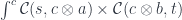
 ![\mathcal{L}\langle s, t\rangle \langle a, b \rangle \cong \int^{c} \mathcal{C}(s, c \times a) \times \mathcal{C}(c, [b, t]) \cong \mathcal{C}(s, [b, t] \times a)](https://s0.wp.com/latex.php?latex=%5Cmathcal%7BL%7D%5Clangle+s%2C+t%5Crangle+%5Clangle+a%2C+b+%5Crangle+%5Ccong+%5Cint%5E%7Bc%7D+%5Cmathcal%7BC%7D%28s%2C+c+%5Ctimes+a%29+%5Ctimes++%5Cmathcal%7BC%7D%28c%2C+%5Bb%2C+t%5D%29+%5Ccong+%5Cmathcal%7BC%7D%28s%2C+%5Bb%2C+t%5D+%5Ctimes+a%29+&bg=ffffff&fg=29303b&s=0&c=20201002)
![\mathcal{C}(s, [b, t]) \times \mathcal{C}(s, a)](https://s0.wp.com/latex.php?latex=%5Cmathcal%7BC%7D%28s%2C+%5Bb%2C+t%5D%29+%5Ctimes+%5Cmathcal%7BC%7D%28s%2C+a%29+&bg=ffffff&fg=29303b&s=0&c=20201002)

 is monoidal, and it has an action defiend on both
  . A category with a monoidal action is called an actegory.
 ).
).
 . It has to be equipped with two additional structure maps—isomorphisms that relate the tensor product
  in
in  to the action in


 , and use the mapping:
![L \colon \mathcal{M} \to [\mathcal{C}, \mathcal{C}]](https://s0.wp.com/latex.php?latex=L+%5Ccolon+%5Cmathcal%7BM%7D+%5Cto+%5B%5Cmathcal%7BC%7D%2C+%5Cmathcal%7BC%7D%5D+&bg=ffffff&fg=29303b&s=0&c=20201002)
![[\mathcal{C}, \mathcal{C}]](https://s0.wp.com/latex.php?latex=%5B%5Cmathcal%7BC%7D%2C+%5Cmathcal%7BC%7D%5D&bg=ffffff&fg=29303b&s=0&c=20201002) , which is naturally equipped with a monoidal structure given by functor composition (and, as we well know, a monad is just a monoid in that category).
, which is naturally equipped with a monoidal structure given by functor composition (and, as we well know, a monad is just a monoid in that category). be a strict monoidal functor, mapping tensor product to functor composition and unit object to identity functor.


 . In that case we have:
 is an object in
 is covariant in
 , we can define the hom-object as:


 in an enriched category must satisfy the composition and identity laws. In an enriched category, composition is a mapping:
 . We get:

 and (twice) the counit of the adjunction
  .
.
 .
. is automatically self-enriched. The copower action
  is equivalent to enrichment over
  , where
  .
.

 by injecting a pair of morphisms from the two hom-sets sharing the same
 ![\mathcal{C}(c \times b, t) \cong \mathcal{C}(c, [b, t])](https://s0.wp.com/latex.php?latex=%5Cmathcal%7BC%7D%28c+%5Ctimes+b%2C+t%29+%5Ccong+%5Cmathcal%7BC%7D%28c%2C+%5Bb%2C+t%5D%29&bg=ffffff&fg=29303b&s=0&c=20201002)
![\int^{c : \mathcal{C}} \mathcal{C}(s, c \times a) \times \mathcal{C}(c, [b, t]) \cong \mathcal{C}(s, [b, t] \times a) \cong \mathcal{C}(s \times b, t) \times \mathcal{C}(s, a)](https://s0.wp.com/latex.php?latex=%5Cint%5E%7Bc+%3A+%5Cmathcal%7BC%7D%7D+%5Cmathcal%7BC%7D%28s%2C+c+%5Ctimes+a%29+%5Ctimes+%5Cmathcal%7BC%7D%28c%2C+%5Bb%2C+t%5D%29+%5Ccong+%5Cmathcal%7BC%7D%28s%2C+%5Bb%2C+t%5D+%5Ctimes+a%29+%5Ccong+%5Cmathcal%7BC%7D%28s+%5Ctimes+b%2C+t%29+%5Ctimes+%5Cmathcal%7BC%7D%28s%2C+a%29&bg=ffffff&fg=29303b&s=0&c=20201002)


 , and further decompose
  , then you can decompose
  . Zooming-in is made possible by the associativity of the tensor product.
 to
to  is the optic
  . Zooming-in is the composition of morphisms.
 in
in 

 is the unit object with respect to the tensor product
  is the identity endofunctor.)
 .
. in
in  in
in 
 . It’s a cross between a coproduct and a trace, as it’s constructed using injections of diagonal elements (with some identifications):
 :
:
 , the base space
  , and a projection, or a display map,
  . The fibers of
  correspond to members of the type family. For instance, the total space, or the bundle, of counted vectors is the list type
  (a free monoid generated by
  ) with the projection
  that returns the length of a list.
 . Counted vectors, for instance, are represented as objects in
  given by pairs
  . Morphisms in the slice category correspond to fibre-wise mappings between bundles.
 has both the left adjoint, the dependent sum
  ; and the right adjoint, the dependent product
  . The base-change functor is defined as a pullback:
 and
and  . In a locally cartesian closed category, this product has the right adjoint, the internal hom in
 .
.


 are objects in the appropriate slice categories.
 on another object
  is given by the pullback:

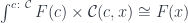
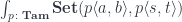
![\cong \int^{\langle C, p \rangle : \mathcal{C}/B} (\mathcal{C}/B)( S, C \times_B A) \times (\mathcal{C}/B)(C , [A', S']_B)](https://s0.wp.com/latex.php?latex=%5Ccong+%5Cint%5E%7B%5Clangle+C%2C+p+%5Crangle+%3A+%5Cmathcal%7BC%7D%2FB%7D+%28%5Cmathcal%7BC%7D%2FB%29%28+S%2C+C+%5Ctimes_B+A%29+%5Ctimes+%28%5Cmathcal%7BC%7D%2FB%29%28C+%2C+%5BA%27%2C+S%27%5D_B%29+&bg=ffffff&fg=29303b&s=0&c=20201002)
![(\mathcal{C}/B)( S, [A', S']_B \times_B A)](https://s0.wp.com/latex.php?latex=%28%5Cmathcal%7BC%7D%2FB%29%28+S%2C+%5BA%27%2C+S%27%5D_B+%5Ctimes_B+A%29+&bg=ffffff&fg=29303b&s=0&c=20201002)
![[A', S']_B](https://s0.wp.com/latex.php?latex=%5BA%27%2C+S%27%5D_B&bg=ffffff&fg=29303b&s=0&c=20201002) in a locally cartesian closed category can be expressed using a dependent product:
in a locally cartesian closed category can be expressed using a dependent product:![\left [\left \langle A' \atop p \right \rangle, \left \langle S' \atop q \right \rangle \right ] \cong \Pi_p \left(p^* \left \langle S' \atop q \right \rangle \right)](https://s0.wp.com/latex.php?latex=%5Cleft+%5B%5Cleft+%5Clangle+A%27+%5Catop+p+%5Cright+%5Crangle%2C+%5Cleft+%5Clangle+S%27+%5Catop+q+%5Cright+%5Crangle+%5Cright+%5D+%5Ccong+%5CPi_p+%5Cleft%28p%5E%2A+%5Cleft+%5Clangle+S%27+%5Catop+q+%5Cright+%5Crangle+%5Cright%29&bg=ffffff&fg=29303b&s=0&c=20201002)
 is the fibration of
  is the right adjoint to the base change functor, and
  is the base-change functor along
 , this is equal to an infinite tuple of functions:
 indexed by
 can be expressed as a fibration
  , with
  , the sum of the fibers. The set of powers of
  , with
  the type of list of
  the function that assigns the length to a list. The monoidal action can then be written using a product (pullback) in the slice category
  :
:
 , which can be used to express the polynomial action:


 is the projection from the cartesian product.
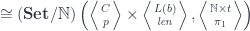
![(\mathbf{Set}/\mathbb{N})\left(\left \langle {C \atop p} \right \rangle, \left[ \left \langle {L(b) \atop \mathit{len}} \right \rangle, \left \langle {\mathbb{N} \times t \atop \pi_1} \right \rangle \right] \right)](https://s0.wp.com/latex.php?latex=%28%5Cmathbf%7BSet%7D%2F%5Cmathbb%7BN%7D%29%5Cleft%28%5Cleft+%5Clangle+%7BC+%5Catop+p%7D+%5Cright+%5Crangle%2C+%5Cleft%5B+%5Cleft+%5Clangle+%7BL%28b%29+%5Catop+%5Cmathit%7Blen%7D%7D+%5Cright+%5Crangle%2C+%5Cleft+%5Clangle+%7B%5Cmathbb%7BN%7D+%5Ctimes+t+%5Catop+%5Cpi_1%7D+%5Cright+%5Crangle+%5Cright%5D+%5Cright%29+&bg=ffffff&fg=29303b&s=0&c=20201002)
 and get:
![O(a, b; s, t) \cong \mathbf{Set} \left( s, U\left( \left[ \left \langle {L(b) \atop \mathit{len}} \right \rangle, \left \langle {\mathbb{N} \times t \atop \pi_1} \right \rangle \right] \times \left \langle {L(a) \atop \mathit{len}} \right \rangle \right) \right)](https://s0.wp.com/latex.php?latex=O%28a%2C+b%3B+s%2C+t%29+%5Ccong+%5Cmathbf%7BSet%7D+%5Cleft%28+s%2C+U%5Cleft%28+%5Cleft%5B+%5Cleft+%5Clangle+%7BL%28b%29+%5Catop+%5Cmathit%7Blen%7D%7D+%5Cright+%5Crangle%2C+%5Cleft+%5Clangle+%7B%5Cmathbb%7BN%7D+%5Ctimes+t+%5Catop+%5Cpi_1%7D+%5Cright+%5Crangle+%5Cright%5D+%5Ctimes+%5Cleft+%5Clangle+%7BL%28a%29+%5Catop+%5Cmathit%7Blen%7D%7D+%5Cright+%5Crangle+%5Cright%29+%5Cright%29+&bg=ffffff&fg=29303b&s=0&c=20201002)


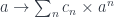
![\int^{c \colon [\mathbb{N}, \mathbf{Set}]} \mathbf{Set}\big(s, \sum_n c_n \times a^n\big) \times \mathbf{Set}\big( \sum_m c_m \times b^m, t\big)](https://s0.wp.com/latex.php?latex=%5Cint%5E%7Bc+%5Ccolon+%5B%5Cmathbb%7BN%7D%2C+%5Cmathbf%7BSet%7D%5D%7D+%5Cmathbf%7BSet%7D%5Cbig%28s%2C+%5Csum_n+c_n+%5Ctimes+a%5En%5Cbig%29+%5Ctimes+%5Cmathbf%7BSet%7D%5Cbig%28+%5Csum_m+c_m+%5Ctimes+b%5Em%2C+t%5Cbig%29+&bg=ffffff&fg=29303b&s=0&c=20201002)
![\int^{c \colon [\mathbb{N}, \mathbf{Set}]} \mathbf{Set}\big(s, \sum_n c_n \times a^n\big) \times \prod_m \mathbf{Set}\big( c_m \times b^m, t\big)](https://s0.wp.com/latex.php?latex=%5Cint%5E%7Bc+%5Ccolon+%5B%5Cmathbb%7BN%7D%2C+%5Cmathbf%7BSet%7D%5D%7D+%5Cmathbf%7BSet%7D%5Cbig%28s%2C+%5Csum_n+c_n+%5Ctimes+a%5En%5Cbig%29+%5Ctimes+%5Cprod_m+%5Cmathbf%7BSet%7D%5Cbig%28+c_m+%5Ctimes+b%5Em%2C+t%5Cbig%29+&bg=ffffff&fg=29303b&s=0&c=20201002)
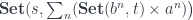
![\int^{c \colon [\mathbb{N}, \mathbf{Set}]} \mathbf{Set}\big(s, \sum_n c_n \times a^n\big) \times \prod_m \mathbf{Set}\big( c_m, \mathbf{Set}( b^m, t)\big)](https://s0.wp.com/latex.php?latex=%5Cint%5E%7Bc+%5Ccolon+%5B%5Cmathbb%7BN%7D%2C+%5Cmathbf%7BSet%7D%5D%7D+%5Cmathbf%7BSet%7D%5Cbig%28s%2C+%5Csum_n+c_n+%5Ctimes+a%5En%5Cbig%29+%5Ctimes+%5Cprod_m+%5Cmathbf%7BSet%7D%5Cbig%28+c_m%2C+%5Cmathbf%7BSet%7D%28+b%5Em%2C+t%29%5Cbig%29+&bg=ffffff&fg=29303b&s=0&c=20201002)
![[\mathbb{N}, \mathbf{Set}]](https://s0.wp.com/latex.php?latex=%5B%5Cmathbb%7BN%7D%2C+%5Cmathbf%7BSet%7D%5D&bg=ffffff&fg=29303b&s=0&c=20201002)
![\int^{c \colon [\mathbb{N}, \mathbf{Set}]} \mathbf{Set}\big(s, \sum_n c_n \times a^n\big) \times [\mathbb{N}, \mathbf{Set}]\big( c_-, \mathbf{Set}( b^-, t)\big)](https://s0.wp.com/latex.php?latex=%5Cint%5E%7Bc+%5Ccolon+%5B%5Cmathbb%7BN%7D%2C+%5Cmathbf%7BSet%7D%5D%7D+%5Cmathbf%7BSet%7D%5Cbig%28s%2C+%5Csum_n+c_n+%5Ctimes+a%5En%5Cbig%29+%5Ctimes+%5B%5Cmathbb%7BN%7D%2C+%5Cmathbf%7BSet%7D%5D%5Cbig%28+c_-%2C+%5Cmathbf%7BSet%7D%28+b%5E-%2C+t%29%5Cbig%29+&bg=ffffff&fg=29303b&s=0&c=20201002)

![F \colon \mathcal{M} \to [\mathcal{C}, \mathcal{C}]](https://s0.wp.com/latex.php?latex=F+%5Ccolon+%5Cmathcal%7BM%7D+%5Cto+%5B%5Cmathcal%7BC%7D%2C+%5Cmathcal%7BC%7D%5D+&bg=ffffff&fg=29303b&s=0&c=20201002)
![G \colon \mathcal{M} \to [\mathcal{D}, \mathcal{D}]](https://s0.wp.com/latex.php?latex=G+%5Ccolon+%5Cmathcal%7BM%7D+%5Cto+%5B%5Cmathcal%7BD%7D%2C+%5Cmathcal%7BD%7D%5D+&bg=ffffff&fg=29303b&s=0&c=20201002)


 into
into  . In physics, we would say that the paths are “invariant” under the transformation, but in category theory we are fine with a one-way mapping.
 , such a mapping exists, then these states are related. There exists a transformation and a pair of morphisms that are secretly used in the path integral to extend the original path.
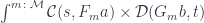
 to
to  by first applying
  and then lifting the two morphisms. The converse is also true: if every path can be extended then such a pair of morphisms must exist.
 can be interpreted both as parameterizing a monoidal action and the residue left over after removing the focus.
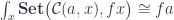
 acting as the unit with respect to taking the end. It takes an
  and returns an
  that we’ve encountered before. They are parameterized by objects in

![\int_{x} \mathbf{Set}\big(\mathcal{C}(a, x), fx\big) = [\mathcal{C}, \mathbf{Set}]\big(\mathcal{C}(a, -), f\big)](https://s0.wp.com/latex.php?latex=%5Cint_%7Bx%7D+%5Cmathbf%7BSet%7D%5Cbig%28%5Cmathcal%7BC%7D%28a%2C+x%29%2C+fx%5Cbig%29+%3D+%5B%5Cmathcal%7BC%7D%2C+%5Cmathbf%7BSet%7D%5D%5Cbig%28%5Cmathcal%7BC%7D%28a%2C+-%29%2C+f%5Cbig%29&bg=ffffff&fg=29303b&s=0&c=20201002)
![[\mathcal{C}, \mathbf{Set}]\big(\mathcal{C}(s, -), \mathcal{C}(a, -) \big)](https://s0.wp.com/latex.php?latex=%5B%5Cmathcal%7BC%7D%2C+%5Cmathbf%7BSet%7D%5D%5Cbig%28%5Cmathcal%7BC%7D%28s%2C+-%29%2C+%5Cmathcal%7BC%7D%28a%2C+-%29+%5Cbig%29&bg=ffffff&fg=29303b&s=0&c=20201002)
 . The result is:
 , so a profunctor is defined a functor from
  to
to  to every pair

![[\mathcal{C}^{op} \times \mathcal{C}, \mathbf{Set}]](https://s0.wp.com/latex.php?latex=%5B%5Cmathcal%7BC%7D%5E%7Bop%7D+%5Ctimes+%5Cmathcal%7BC%7D%2C+%5Cmathbf%7BSet%7D%5D&bg=ffffff&fg=29303b&s=0&c=20201002) . We can immediately apply the double Yoneda identity to it to get:
. We can immediately apply the double Yoneda identity to it to get:


 . Let me explain.
![[\mathcal{C}, \mathbf{Set}]](https://s0.wp.com/latex.php?latex=%5B%5Cmathcal%7BC%7D%2C+%5Cmathbf%7BSet%7D%5D&bg=ffffff&fg=29303b&s=0&c=20201002) and endow it with some structure, resulting in another functor category
and endow it with some structure, resulting in another functor category  . It means that there is a (higher-order) forgetful functor
 ![U \colon \mathcal{T} \to [\mathcal{C}, \mathbf{Set}]](https://s0.wp.com/latex.php?latex=U+%5Ccolon+%5Cmathcal%7BT%7D+%5Cto+%5B%5Cmathcal%7BC%7D%2C+%5Cmathbf%7BSet%7D%5D&bg=ffffff&fg=29303b&s=0&c=20201002) that forgets this additional structure. We’ll also assume that there is the right adjoint functor
that forgets this additional structure. We’ll also assume that there is the right adjoint functor 
 is a functor in
![\int_{x \colon C} \mathbf{Set}\big(\mathcal{C}(a, x), (U f) x\big) = [\mathcal{C}, \mathbf{Set}]\big(\mathcal{C}(a, -), U f\big)](https://s0.wp.com/latex.php?latex=%5Cint_%7Bx+%5Ccolon+C%7D+%5Cmathbf%7BSet%7D%5Cbig%28%5Cmathcal%7BC%7D%28a%2C+x%29%2C+%28U+f%29+x%5Cbig%29+%3D+%5B%5Cmathcal%7BC%7D%2C+%5Cmathbf%7BSet%7D%5D%5Cbig%28%5Cmathcal%7BC%7D%28a%2C+-%29%2C+U+f%5Cbig%29&bg=ffffff&fg=29303b&s=0&c=20201002)
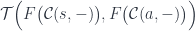
![[\mathcal{C}, \mathbf{Set}]\big(\mathcal{C}(a, -), U f\big) \cong \mathcal{T}\Big(F\big(\mathcal{C}(a, -)\big), f\Big)](https://s0.wp.com/latex.php?latex=%5B%5Cmathcal%7BC%7D%2C+%5Cmathbf%7BSet%7D%5D%5Cbig%28%5Cmathcal%7BC%7D%28a%2C+-%29%2C+U+f%5Cbig%29+%5Ccong+%5Cmathcal%7BT%7D%5CBig%28F%5Cbig%28%5Cmathcal%7BC%7D%28a%2C+-%29%5Cbig%29%2C+f%5CBig%29&bg=ffffff&fg=29303b&s=0&c=20201002)

![[\mathcal{C}, \mathbf{Set}] \Big( \mathcal{C}(s, -), (U \circ F)\big(\mathcal{C}(a, -)\big) \Big)](https://s0.wp.com/latex.php?latex=%5B%5Cmathcal%7BC%7D%2C+%5Cmathbf%7BSet%7D%5D+%5CBig%28+%5Cmathcal%7BC%7D%28s%2C+-%29%2C+%28U+%5Ccirc+F%29%5Cbig%28%5Cmathcal%7BC%7D%28a%2C+-%29%5Cbig%29+%5CBig%29+&bg=ffffff&fg=29303b&s=0&c=20201002)


 on the hom-functor
  . This is a monad in the functor category


 :
:
 .
.
 are given by natural transformations:
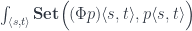


 with
with 
 (or
(or  stands for the set of arrows from
  in
in  stands for a set of functions from
  or, in Haskell
  can be expressed using the end notation:
 , it becomes a functor, which is called a representable functor—the object
![[\mathcal{C},\mathbf{Set}]](https://s0.wp.com/latex.php?latex=%5B%5Cmathcal%7BC%7D%2C%5Cmathbf%7BSet%7D%5D&bg=ffffff&fg=29303b&s=0&c=20201002) . A hom-set in that category is a set of natural transformations between two functors which, as we’ve seen, can be expressed as an end:
. A hom-set in that category is a set of natural transformations between two functors which, as we’ve seen, can be expressed as an end: \cong \int_x \mathbf{Set}(f x, g x)](https://s0.wp.com/latex.php?latex=%5B%5Cmathcal%7BC%7D%2C%5Cmathbf%7BSet%7D%5D%28f%2C+g%29+%5Ccong+%5Cint_x+%5Cmathbf%7BSet%7D%28f+x%2C+g+x%29+&bg=ffffff&fg=29303b&s=0&c=20201002)
, [\mathcal{C},\mathbf{Set}](h, f)\big) \cong [\mathcal{C},\mathbf{Set}](h, g)](https://s0.wp.com/latex.php?latex=%5Cint_f+%5Cmathbf%7BSet%7D%5Cbig%28+%5B%5Cmathcal%7BC%7D%2C%5Cmathbf%7BSet%7D%5D%28g%2C+f%29%2C+%5B%5Cmathcal%7BC%7D%2C%5Cmathbf%7BSet%7D%5D%28h%2C+f%29%5Cbig%29+%5Ccong+%5B%5Cmathcal%7BC%7D%2C%5Cmathbf%7BSet%7D%5D%28h%2C+g%29+&bg=ffffff&fg=29303b&s=0&c=20201002)
 is all we need to finish the proof.

 corresponds to the function type
  . This is just saying that a function of two arguments is equivalent to a function returning a function.
 and
and  , where
  and
and  are some higher-order functors from
 , [\mathcal{C},\mathbf{Set}](L_t s, f)\big) \cong [\mathcal{C},\mathbf{Set}](L_t s, L_b a)](https://s0.wp.com/latex.php?latex=%5Cint_f+%5Cmathbf%7BSet%7D%5Cbig%28+%5B%5Cmathcal%7BC%7D%2C%5Cmathbf%7BSet%7D%5D%28L_b+a%2C+f%29%2C+%5B%5Cmathcal%7BC%7D%2C%5Cmathbf%7BSet%7D%5D%28L_t+s%2C+f%29%5Cbig%29+%5Ccong+%5B%5Cmathcal%7BC%7D%2C%5Cmathbf%7BSet%7D%5D%28L_t+s%2C+L_b+a%29+&bg=ffffff&fg=29303b&s=0&c=20201002)
 and
and  that go in the opposite direction from


 \cong \mathcal{C}(a, R_b f) = \mathcal{C}(a, f b)](https://s0.wp.com/latex.php?latex=%5B%5Cmathcal%7BC%7D%2C%5Cmathbf%7BSet%7D%5D%28L_b+a%2C+f%29+%5Ccong+%5Cmathcal%7BC%7D%28a%2C+R_b+f%29+%3D+%5Cmathcal%7BC%7D%28a%2C+f+b%29&bg=ffffff&fg=29303b&s=0&c=20201002)


 translates to the function type


 . The breakthrough came with the realization that, if


 defined by the unique property of leaving things alone


 happens to have a similar decomposition


 .
.
