Abstract: I present a uniform derivation of profunctor optics: isos, lenses, prisms, and grates based on the Yoneda lemma in the (enriched) profunctor category. In particular, lenses and prisms correspond to Tambara modules with the cartesian and cocartesian tensor product.
This blog post is the result of a collaboration between many people. The categorical profunctor picture solidified after long discussions with Edward Kmett. A lot of the theory was developed in exchanges on the Lens IRC channel between Russell O’Connor, Edward Kmett and James Deikun. They came up with the idea to use the Pastro functor to freely generate Tambara modules, which was the missing piece that completed the picture.
My interest in lenses started long time ago when I first made the connection between the universal quantification over functors in the van Laarhoven representation of lenses and the Yoneda lemma. Since I was still learning the basics of category theory, it took me a long time to find the right language to make the formal derivation. Unbeknownst to me Mauro Jaskellioff and Russell O’Connor independently had the same idea and they published a paper about it soon after I published my blog. But even though this solved the problem of lenses, prisms still seemed out of reach of the Yoneda lemma. Prisms require a more general formulation using universal quantification over profunctors. I was able to put a dent in it by deriving Isos from profunctor Yoneda, but then I was stuck again. I shared my ideas with Russell, who reached for help on the IRC channel, and a Haskell proof of concept was quickly established. Two years later, after a brainstorm with Edward, I was finally able to gather all these ideas in one place and give them a little categorical polish.
Yoneda Lemma
The starting point is the Yoneda lemma, which states that the set of natural transformations between the hom-functor C(a, -) in the category C and an arbitrary functor f from C to Set is (naturally) isomorphic with the set f a:
[C, Set](C(a, -), f) ≅ f a
Here, f is a member of the functor category [C, Set], where natural transformation form hom-sets.
The set of natural transformations may be represented as an end, leading to the following formulation of the Yoneda lemma:
∫x Set(C(a, x), f x) ≅ f a
This notation makes the object x explicit, which is often very convenient. It can be easily translated to Haskell, by replacing the end with the universal quantifier. We get:
forall x. (a -> x) -> f x ≅ f a
A special case of the Yoneda lemma replaces the functor f with a hom-functor in C:
f x = C(b, x)
and we get:
∫x Set(C(a, x), C(b, x)) ≅ C(b, a)
This form of the Yoneda lemma is useful in showing the Yoneda embedding, which states that any category C can be fully and faithfully embedded in the functor category [C, Set]. The embedding is a functor, and the above formula defines its action on morphisms.
We will be interested in using the Yoneda lemma in the functor category. We simply replace C with [C, Set] in the previous formula, and do some renaming of variables:
∫f Set([C, Set](g, f), [C, Set](h, f)) ≅ [C, Set](h, g)
The hom-sets in the functor category are sets of natural transformations, which can be rewritten using ends:
∫f Set(∫x Set(g x, f x), ∫x Set(h x, f x))
≅ ∫x Set(h x, g x)
Adjunctions
This is a short recap of adjunctions. We start with two functors going between two categories C and D:
L :: C -> D
R :: D -> C
We say that L is left adjoint to R iff there is a natural isomorphism between hom-sets:
D(L x, y) ≅ C(x, R y)
In particular, we can define an adjunction in a functor category [C, Set]. We start with two higher order (endo-) functors:
L :: [C, Set] -> [C, Set]
R :: [C, Set] -> [C, Set]
We say that L is left adjoint to R iff there is a natural isomorphism between two sets of natural transformations:
[C, Set](L f, g) ≅ [C, Set](f, R g)
where f and g are functors from C to Set. We can rewrite natural transformations using ends:
∫x Set((L f) x, g x) ≅ ∫x Set(f x, (R g) x)
In Haskell, you may think of f and g as type constructors (with the corresponding Functor instances), in which case L and R are types that are parameterized by these type constructors (similar to how the monad or functor classes are).
Yoneda with Adjunction
Here’s a little trick. Since the fixed objects in the formula for Yoneda embedding are arbitrary, we can pick them to be images of other objects under some functor L that we know is left adjoint to another functor R:
∫x Set(D(L a, x), D(L b, x)) ≅ D(L b, L a)
Using the adjunction, this is isomorphic to:
∫x Set(C(a, R x), C(b, R x)) ≅ C(b, (R ∘ L) a)
Notice that the composition R ∘ L of adjoint functors is a monad in C. Let’s write this monad as Φ.
The interesting case is the adjunction between a forgetful functor U and a free functor F. We get:
∫x Set(C(a, U x), C(b, U x)) ≅ C(b, Φ a)
The end is taken over x in a category D that has some additional structure (we’ll see examples of that later); but the hom-sets are in the underlying simpler category C, which is the target of the forgetful functor U.
The Yoneda-with-adjunction formula generalizes to the category of functors:
∫f Set(∫x Set((L g) x, f x), ∫x Set((L h) x, f x))
≅ ∫x Set((L h) x, (L g) x)
leading to:
∫f Set(∫x Set((g x, (R f) x), ∫x Set(h x, (R f) x))
≅ ∫x Set(h x, (Φ g) x)
Here, Φ is the monad R ∘ L in the category of functors.
An interesting special case is when we substitute hom-functors for g and h:
g x = C(a, x)
h x = C(s, x)
We get:
∫f Set(∫x Set((C(a, x), (R f) x), ∫x Set(C(s, x), (R f) x))
≅ ∫x Set(C(s, x), (Φ C(a, -)) x)
We can then use the regular Yoneda lemma to “integrate over x” and reduce it down to:
∫f Set((R f) a, (R f) s)) ≅ (Φ C(a, -)) s
Again, we are particularly interested in the forgetful/free adjunction:
∫f Set((U f) a, (U f) s)) ≅ (Φ C(a, -)) s
with the monad:
Φ = U ∘ F
The simplest application of this identity is when the functors in question are identity functors. We get:
∫f Set(f a, f s)) ≅ C(a, s)
In Haskell this becomes:
forall f. Functor f => f a -> f s ≅ a -> s
You may think of this formula as defining the trivial kind of optic that simply turns a to s.
Profunctors
Profunctors are just functors from a product category Cop×D to Set. All the results from the last section can be directly applied to the profunctor category [Cop×D, Set]. Keep in mind that morphisms in this category are natural transformations between profunctors. Here’s the key formula:
∫p Set((U p)<a, b>, (U p)<s, t>)) ≅ (Φ (Cop×D)(<a, b>, -)) <s, t>
I have replaced a with a pair <a, b> and s with a pair <s, t>. The end is taken over all profunctors that exhibit some structure that U forgets, and F freely creates. Φ is the monad U ∘ F. It’s a monad that acts on profunctors to produce other profunctors.
Notice that a hom-set in the category Cop×D is a set of pairs of morphisms:
<f, g> :: (Cop×D)(<a, b>, <s, t>)
f :: s -> a
g :: b -> t
the first one going in the opposite direction.
The simplest application of this identity is when we don’t impose any constraints on the profunctors, in which case Φ is the identity monad. We get:
∫p Set(p <a, b>, p <s, t>) ≅ (Cop×D)(<a, b>, <s, t>)
Haskell translation of this formula gives the well-known representation of Iso:
forall p. Profunctor p => p a b -> p s t ≅ Iso s t a b
where:
data Iso s t a b = Iso (s -> a) (b -> t)
Interesting things happen when we impose more structure on our profunctors.
Enriched Categories
First, let’s generalize profunctors to work on enriched categories. We start with some monoidal category V whose objects serve as hom-objects in an enriched category A. The category V will essentially replace Set in our constructions. For instance, we’ll work with profunctors that are enriched functors from the (enriched) product category to V:
p :: Aop ⊗ A -> V
Notice that we use a tensor product of categories. The objects in such a category are pairs of objects, and the hom-objects are tensor products of individual hom-objects. The definition of composition in a product category requires that the tensor product in V be symmetric (up to isomorphism).
For such profunctors, there is a suitable generalization of the end:
∫x p x x
It’s an object in V together with a V-natural family of projections:
pry :: ∫x p x x -> p y y
We can formulate the Yoneda lemma in an enriched setting by considering enriched functors from A to V. We get the following generalization:
∫x [A(a, x), f x] ≅ f a
Notice that A(a, x) is now an object of V — the hom-object from a to x. The notation [v, w] generalizes the internal hom. It is defined as the right adjoint to the tensor product in V:
V(x ⊗ v, w) ≅ V(x, [v, w])
We are assuming that V is closed, so the internal hom is defined for every pair of objects.
Enriched functors, or V-functors, between two enriched categories C and D form a functor category [C, D] that is itself enriched over V. The hom-object between two functors f and g is given by the end:
[C, D](f, g) = ∫x D(f x, g x)
We can therefore use the Yoneda lemma in a category of enriched functors, or in the category of enriched profunctors. Therefore the result of the previous section holds in the enriched setting as well:
∫p [(U p)<a, b>, (U p)<s, t>] ≅ (Φ (Aop⊗A)(<a, b>, -)) <s, t>
with the understanding that:
(Aop⊗A)(<a, b>, -))
is an enriched hom functor mapping pairs of objects in A to objects in V, plus the appropriate action on hom-objects. This hom-functor is the profunctor on which Φ acts.
Tambara Modules
An enriched category A may have a monoidal structure of its own. We’ll use the same tensor product notation for its structure as we did for the underlying monoidal category V. There is also a tensorial unit object i in A.
A Tambara module is a V-functor p from Aop⊗A to V, which transforms under the tensor action of A according to a family of morphisms, natural in all three arguments:
α a x y :: p x y -> p (a ⊗ x) (a ⊗ y)
Notice that these are morphisms in the underlying category V, which is also the target of the profunctor.
We impose the usual unit law:
α i x y = id
and associativity:
α a⊗b x y = α a b⊗x b⊗y ∘ α b x y
Strictly speaking one can separately define left and right action but, for simplicity, we’ll assume that the product is symmetric (up to isomorphism).
The intuition behind Tambara modules is that some of the profunctor values are not independent of others. Once we have calculated p x y, we can obtain the value of p at any of the points on the path <a⊗x, a⊗y> by applying α.
Tambara modules form a category that’s enriched over V. The construction of this enrichment is non-trivial. The hom-object between two profunctors p and q in a category of profunctors is given by the end:
[Aop⊗A, V](p, q) = ∫<x y> V(p x y, q x y)
This object generalizes the set of natural transformations. Conceptually, not all natural transformation preserve the Tambara structure, so we have to define a subobject of this hom-object that does. The intuition is that the end is a generalized product of its components. It comes equipped with projections. For instance, the projection pr<x,y> picks the component:
V(p x y, q x y)
But there is also a projection pr<a⊗x, a⊗y> that picks:
V(p a⊗x a⊗y, q a⊗x a⊗y)
from the same end. These two objects are not completely independent, because they can both be transformed into the same object. We have:
V(id, αa) :: V(p x y, q x y) -> V(p x y, q a⊗x a⊗y)
V(αa, id) :: V(a⊗x a⊗y, q a⊗x a⊗y) -> V(p x y, q a⊗x a⊗y)
We are using the fact that the mapping:
<v, w> -> V(v, w)
is itself a profunctor Vop×V -> V, so it can be used to lift pairs of morphisms in V.
Now, given any triple a, x, and y, we want the two paths to be equivalent, which means finding the equalizer between each pair of morphisms:
V(id, αa) ∘ pr<x, y>
V(αa, id) ∘ pr<a⊗x, a⊗y>

Since we want our hom-object to satisfy the above condition for any triple, we have to construct it as an intersection of all those equalizers. Here, an intersection means an object of V together with a family of monomorphisms, each embedding it into a particular equalizer.
It’s possible to construct a forgetful functor from the Tambara category to the category of profunctors [Aop⊗A, V]. It forgets the existence of α and it maps hom-objects between the two categories. Composition in the Tambara category is defined is such a way as to be compatible with this forgetful functor.
The fact that Tambara modules form a category is important, because we want to be able to use the Yoneda lemma in that category.
Tambara Optics
The key observation is that the forgetful functor from the Tambara category has a left adjoint, and that their composition forms a monad in the category of profunctors. We’ll plug this monad into our general formula.
The construction of this monad starts with a comonad that is given by the following end:
(Θ p) s t = ∫c p (c⊗s) (c⊗t)
For a given profunctor p, this comonad builds a new profunctor that is essentially a gigantic product of all values of this profunctor “shifted” by tensoring its arguments with all possible objects c.
The monad we are interested in is the left adjoint to this comonad (calculated using a Kan extension):
(Φ p) s t = ∫ c x y A(s, c⊗x) ⊗ A(c⊗y, t) ⊗ p x y
Notice that we have two separate tensor products in this formula: one in V, between the hom-objects and the profunctor, and one in A, under the hom-objects. This monad takes an arbitrary profunctor p and produces a new profunctor Φ p.
We can now use our earlier formula:
∫p [(U p)<a, b>, (U p)<s, t>)] ≅ (Φ (Aop⊗A)(<a, b>, -)) <s, t>
inside the Tambara category. To calculate the right hand side, let’s evaluate the action of Φ on the hom-profunctor:
(Φ (Aop⊗A)(<a, b>, -)) <s, t>
= ∫ c x y A(s, c⊗x) ⊗ A(c⊗y, t) ⊗ (Aop⊗A)(<a, b>, <x, y>)
We can “integrate over” x and y using the Yoneda lemma to get:
∫ c A(s, c⊗a) ⊗ A(c⊗b, t)
We get the following result:
∫p [(U p)<a, b>, (U p)<s, t>)] ≅ ∫ c A(s, c⊗a) ⊗ A(c⊗b, t)
where the end on the left is taken over all Tambara modules, and U is the forgetful functor from the Tambara category to the category of profunctors.
If the category in question is closed, we can use the adjunction:
A(c⊗b, t) ≅ A(c, [b, t])
and “perform the integration” over c to arrive at the set/get formulation:
∫ c A(s, c⊗a) ⊗ A(c, [b, t]) ≅ A(s, [b, t]⊗a)
It corresponds to the familiar Haskell lens type:
(s -> b -> t, s -> a)
(This final trick doesn’t work for prisms, because there is no right adjoint to Either.)
Haskell Translation
A Tambara module is parameterized by the choice of the tensor product ten. We can write a general definition:
class (Profunctor p) => TamModule (ten :: * -> * -> *) p where
leftAction :: p a b -> p (c `ten` a) (c `ten` b)
rightAction :: p a b -> p (a `ten` c) (b `ten` c)
This can be further specialized for two obvious monoidal structures: product and sum:
type TamProd p = TamModule (,) p
type TamSum p = TamModule Either p
The former is equivalent to what it called a Strong (or Cartesian) profunctor in Haskell, the latter is equivalent to a Choice (or Cocartesian) profunctor.
Replacing ends and coends with universal and existential quantifiers in Haskell, our main formula becomes (pseudocode):
forall p. TamModule ten p => p a b -> p s t
≅ exists c. (s -> c `ten` a, c `ten` b -> t)
The two sides of the isomorphism can be defined as the following data structures:
type TamOptic ten s t a b
= forall p. TamModule ten p => p a b -> p s t
data Optic ten s t a b
= forall c. Optic (s -> c `ten` a) (c `ten` b -> t)
Chosing product for the tensor, we recover two equivalent definitions of a lens:
type Lens s t a b = forall p. Strong p => p a b -> p s t
data Lens s t a b =
forall c. Lens (s -> (c, a)) ((c, b) -> t)
Chosing the coproduct, we get:
type Prism s t a b = forall p. Choice p => p a b -> p s t
data Prism s t a b =
forall c. Prism (s -> Either c a)
                (Either c b -> t)
These are the well-known existential representations of lenses and prisms.
The monad Φ (or, equivalently, the free functor that generates Tambara modules), is known in Haskell under the name Pastro for product, and Copastro for coproduct:
data Pastro p a b where
  Pastro :: ((y, z) -> b) -> p x y -> (a -> (x, z))
            -> Pastro p a b
data Copastro p a b where
  Copastro :: (Either y z -> b) -> p x y -> (a -> Either x z)
            -> Copastro p a b
They are the left adjoints of Tambara and Cotambara, respectively:
newtype Tambara p a b = Tambara forall c. p (a, c) (b, c)
newtype Cotambara p a b = Cotambara forall c. p (Either a c) (Either b c)
which are special cases of the comonad Θ.
Discussion
It’s interesting that the work on Tambara modules has relevance to Haskell optics. It is, however, just one example of an even larger pattern.
The pattern is that we have a family of transformations in some category A. These transformations can be used to select a class of profunctors that have simple transformation laws. Using a tensor product in a monoidal category to transform objects, in essence “multiplying” them, is just one example of such symmetry. A more general pattern involves a family of transformations f that is closed under composition and includes a unit. We specify a transformation law for profunctors:
class Profunctor p => Related p where
    α f a b :: forall f. Trans f => p a b -> p (f a) (f b)
This requirement picks a class of profunctors that we call Related.
Why are profunctors relevant as carriers of symmetry? It’s because they generalize a relationship between objects. The profunctor transformation law essentially says that if two objects a and b are related through p then so are the transformed objects; and that there is a function α that relates the proofs of this relationship. This is in the spirit of profunctors as proof-relevant relations.
As an analogy, imagine that we are comparing people, and the transformation we’re interested in is aging. We notice that family relationships remain invariant under aging: if a is a sibling of b, they will remain siblings as they age. This is not true about other relationships, for instance being a boss of another person. But family bonds are not the only ones that survive the test of time. Another such relation is being older or younger than the other person.
Now imagine that you pick four people at random points in time and you find out that any time-invariant relation between two of them, a and b, also holds between s and t. You have to conclude that there is some connection between s and age-adjusted a, and between age-adjusted b and t. In other words there exists a time shift that transforms one pair to another.
Considering all possible relations from the class Related corresponds to taking the end over all profunctors from this class:
type Optic p s t a b = forall p. Related p =>
    p a b -> p s t
The end is a generalization of a product, so it’s enough that one of the components is empty for the whole end to be empty. It means that, for a particular choice of the four types a, b, s, and t, we have to be able to construct a whole family of morphisms, one for every p. We have seen that this end exists only if the four types are connected in a very peculiar way — for instance, if a and b are somehow embedded in s and t.
In the simplest case, we may choose the four types to be related by the transformation:
s = f a
t = f b
For these types, we know that the end exists:
forall p. Related p =>
    p a b -> p s t
because there is a family of appropriate morphisms: our αf a b. In general, though, we can get away with weaker connection.
Let’s look at an example of a family of transformations generated by pairing with arbitrary type c:
fc a = (c, a)
Profunctors that respect these transformations are Tambara modules over a cartesian product (or, in lens parlance, Strong profunctors). For the choice:
s = (c, a)
t = (c, b)
the end in question trivially exists. As we’ve seen, we can weaken these conditions. It’s enough that one way (lax) transformations exist:
s -> (c, a)
t <- (c, b)
These morphisms assert that s can be split into a pair, and that t can be constructed from a pair (but not the other way around).
Other Optics
With the understanding that optics may be defined using a family of transformations, we can analyze another optic called the Grate. It’s based on the following family:
type Reader e a = e -> a
Notice that, unlike the case of Tambara modules, this family is parameterized by a contravariant parameter e.
We are interested in profunctors that transform under these transformations:
class Profunctor p => Closed p where
    closed :: p a b -> p (x -> a) (x -> b)
They let us form the optic:
type Grate s t a b = forall p. Closed p => p a b -> p s t
It turns out that there is a profunctor functor that freely generates Closed profunctors. We have the obvious comonad:
newtype Closure p a b = Closure forall x. p (x -> a) (x -> b)
and its adjoint monad:
data Environment p u v where
  Environment :: ((c -> y) -> v) -> p x y -> (u -> (c -> x))
                 -> Environment p a b
or, in categorical notation:
(Φ p) u v = ∫ c x y A([c, y], v) ⊗ p x y ⊗ A(u, [c, x])
Using our construction, we apply this monad to the hom-profunctor:
(Φ (Aop⊗A)(<a, b>, -)) <s, t>
= ∫ c x y A([c, y], t) ⊗ (Aop⊗A)(<a, b>, <x, y>) ⊗ A(s, [c, x])
≅ ∫ c A([c, b], t) ⊗ A(s, [c, a])
Translating it back to Haskell, we get a representation of Grate as an existential type:
Grate s t a b = forall c. Grate ((c -> b) -> t) (s -> (c -> a))
This is very similar to the existential representation of a lens or a prism. It has the intuitive interpretation that s can be thought of as a container of a‘s indexed by some hidden type c.
We can also “perform the integration” using the Yoneda lemma, internal-hom-adjunction, and the symmetry of the product:
∫ c A([c, b], t) ⊗ A(s, [c, a])
≅ ∫ c A([c, b], t) ⊗ A(s ⊗ c, a)
≅ ∫ c A([c, b], t) ⊗ A(c, [s, a])
≅ A([[s, a], b], t)
to get the more familiar form:
Grate s t a b ≅ ((s -> a) -> b) -> t
Conclusion
I find it fascinating that constructions that were first discovered in Haskell to make Haskell’s optics composable have their categorical counterparts. This was not at all obvious, if only because some of them use parametricity arguments. Parametricity is the property of the language, not easily translatable to category theory. Now we know that the profunctor formulation of isos, lenses, prisms, and grates follows from the Yoneda lemma. The work is not complete yet. I haven’t been able to derive the same formulation for traversals, which combine two different tensor products plus some monoidal constraints.
Bibliography
- Haskell lens library, Edward Kmett
- Distributors on a tensor category, D. Tambara
- Doubles for monoidal categories, Craig Pastro, Ross Street
- Profunctor optics, Modular data accessors,
Matthew Pickering, Jeremy Gibbons, and Nicolas Wu
- CPS based functional references, Twan van Laarhoven
- Isomorphism lenses, Twan van Laarhoven
- Theorem for Second-Order Functionals, Mauro Jaskellioff and Russell O’Connor


 ) and existential quantifiers (there exists,
  ).
).

 is written as
  . The resulting optic has two possible residues,
 (I’ll use the same notation for both actions). The actions are composed using the tensor product in
 into the action of some
  from the action of the same
 and
and  can be treated as fibers over the set
  , while the sets
  and
and  are fibers over a different set
  .
. , that is co-presheaves. For instance
  of a discrete category
  . The products over
  are fibrated over two different sets. I have previously interpreted them as
![[\mathcal C, Set ]](https://s0.wp.com/latex.php?latex=%5B%5Cmathcal+C%2C+Set+%5D&bg=ffffff&fg=29303b&s=0&c=20201002) behaves, in many respects, like a vector space. For instance, it has a “basis” consisting of representable functors
behaves, in many respects, like a vector space. For instance, it has a “basis” consisting of representable functors  ; in the sense that any co-presheaf is as a colimit of representables. Moreover, colimit-preserving functors between co-presheaf categories are very similar to linear transformations between vector spaces. Of particular interest are functors that are left adjoint to some other functors, since left adjoints preserve colimits.
 and
and  and another with
  and
and  . Rectangular matrices
 is the transposed matrix. Transposition here serves as an analog of adjunction.
 as discrete categories. We have:
![a, b \colon [\mathcal N, \mathbf{Set}]](https://s0.wp.com/latex.php?latex=a%2C+b+%5Ccolon+%5B%5Cmathcal+N%2C+%5Cmathbf%7BSet%7D%5D+&bg=ffffff&fg=29303b&s=0&c=20201002)
![s, t \colon [\mathcal K, \mathbf{Set}]](https://s0.wp.com/latex.php?latex=s%2C+t+%5Ccolon+%5B%5Cmathcal+K%2C+%5Cmathbf%7BSet%7D%5D+&bg=ffffff&fg=29303b&s=0&c=20201002)
 is a functor between categories of co-presheaves:
![c \colon [\mathcal N, \mathbf{Set}] \to [\mathcal K, \mathbf{Set}]](https://s0.wp.com/latex.php?latex=c+%5Ccolon+%5B%5Cmathcal+N%2C+%5Cmathbf%7BSet%7D%5D+%5Cto+%5B%5Cmathcal+K%2C+%5Cmathbf%7BSet%7D%5D+&bg=ffffff&fg=29303b&s=0&c=20201002)
 .
.![[\mathcal K, \mathbf{Set}] (c \bullet a, t) \cong [\mathcal N, \mathbf{Set}] (a, c^{\dagger} \bullet t)](https://s0.wp.com/latex.php?latex=%5B%5Cmathcal+K%2C+%5Cmathbf%7BSet%7D%5D+%28c+%5Cbullet+a%2C+t%29+%5Ccong+%5B%5Cmathcal+N%2C+%5Cmathbf%7BSet%7D%5D+%28a%2C+c%5E%7B%5Cdagger%7D+%5Cbullet+t%29+&bg=ffffff&fg=29303b&s=0&c=20201002)
![c^{\dagger} \colon [\mathcal K, \mathbf{Set}] \to [\mathcal N, \mathbf{Set}]](https://s0.wp.com/latex.php?latex=c%5E%7B%5Cdagger%7D+%5Ccolon+%5B%5Cmathcal+K%2C+%5Cmathbf%7BSet%7D%5D+%5Cto+%5B%5Cmathcal+N%2C+%5Cmathbf%7BSet%7D%5D+&bg=ffffff&fg=29303b&s=0&c=20201002)
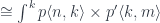
![\mathcal{O}\langle a, b\rangle \langle s, t \rangle = \int^{c} [\mathcal K, \mathbf{Set}] \left(s, c \bullet a \right) \times [\mathcal K, \mathbf{Set}] \left(c \bullet b, t \right)](https://s0.wp.com/latex.php?latex=%5Cmathcal%7BO%7D%5Clangle+a%2C+b%5Crangle+%5Clangle+s%2C+t+%5Crangle+%3D+%5Cint%5E%7Bc%7D+%5B%5Cmathcal+K%2C+%5Cmathbf%7BSet%7D%5D+%5Cleft%28s%2C++c+%5Cbullet+a+%5Cright%29+%5Ctimes+%5B%5Cmathcal+K%2C+%5Cmathbf%7BSet%7D%5D+%5Cleft%28c+%5Cbullet+b%2C+t+%5Cright%29+&bg=ffffff&fg=29303b&s=0&c=20201002)

 is a representable co-presheaf.
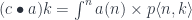
 :
:![\int^{p} [\mathcal K, \mathbf{Set}] \left(s, \int^{n} a(n) \times p \langle n, - \rangle \right) \times [\mathcal K, \mathbf{Set}] \left(\int^{n'} b(n') \times p \langle n', - \rangle, t \right)](https://s0.wp.com/latex.php?latex=%5Cint%5E%7Bp%7D+%5B%5Cmathcal+K%2C+%5Cmathbf%7BSet%7D%5D+%5Cleft%28s%2C++%5Cint%5E%7Bn%7D+a%28n%29+%5Ctimes+p+%5Clangle+n%2C+-+%5Crangle+%5Cright%29+%5Ctimes+%5B%5Cmathcal+K%2C+%5Cmathbf%7BSet%7D%5D+%5Cleft%28%5Cint%5E%7Bn%27%7D+b%28n%27%29+%5Ctimes+p+%5Clangle+n%27%2C+-+%5Crangle%2C+t+%5Cright%29+&bg=ffffff&fg=29303b&s=0&c=20201002)
![c \colon [\mathcal N, \mathbf{Set}] \to [\mathcal K, \mathbf{Set}]](https://s0.wp.com/latex.php?latex=c+%5Ccolon++%5B%5Cmathcal+N%2C+%5Cmathbf%7BSet%7D%5D+%5Cto+%5B%5Cmathcal+K%2C+%5Cmathbf%7BSet%7D%5D+&bg=ffffff&fg=29303b&s=0&c=20201002)
![c' \colon [\mathcal K, \mathbf{Set}] \to [\mathcal M, \mathbf{Set}]](https://s0.wp.com/latex.php?latex=c%27+%5Ccolon++%5B%5Cmathcal+K%2C+%5Cmathbf%7BSet%7D%5D+%5Cto+%5B%5Cmathcal+M%2C+%5Cmathbf%7BSet%7D%5D+&bg=ffffff&fg=29303b&s=0&c=20201002)
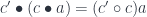
 corresponding to
  is given by:

 and
and  . The first one tells us that there exists a
 ![l_c (s, a ) = [\mathcal K, \mathbf{Set}] \left(s, c \bullet a \right)](https://s0.wp.com/latex.php?latex=l_c+%28s%2C++a+%29+%3D+%5B%5Cmathcal+K%2C+%5Cmathbf%7BSet%7D%5D+%5Cleft%28s%2C++c+%5Cbullet+a+%5Cright%29+&bg=ffffff&fg=29303b&s=0&c=20201002)
![r_c (b, t) = [\mathcal K, \mathbf{Set}] \left(c \bullet b, t \right)](https://s0.wp.com/latex.php?latex=r_c+%28b%2C+t%29+%3D+%5B%5Cmathcal+K%2C+%5Cmathbf%7BSet%7D%5D+%5Cleft%28c+%5Cbullet+b%2C+t+%5Cright%29+&bg=ffffff&fg=29303b&s=0&c=20201002)
 and a pair:
![l'_{c'} (a, a' ) = [\mathcal K, \mathbf{Set}] \left(a, c' \bullet a' \right)](https://s0.wp.com/latex.php?latex=l%27_%7Bc%27%7D+%28a%2C++a%27+%29+%3D+%5B%5Cmathcal+K%2C+%5Cmathbf%7BSet%7D%5D+%5Cleft%28a%2C++c%27+%5Cbullet+a%27+%5Cright%29+&bg=ffffff&fg=29303b&s=0&c=20201002)
![r'_{c'} (b', b) = [\mathcal K, \mathbf{Set}] \left(c' \bullet b', b \right)](https://s0.wp.com/latex.php?latex=r%27_%7Bc%27%7D+%28b%27%2C+b%29+%3D+%5B%5Cmathcal+K%2C+%5Cmathbf%7BSet%7D%5D+%5Cleft%28c%27+%5Cbullet+b%27%2C+b+%5Cright%29+&bg=ffffff&fg=29303b&s=0&c=20201002)
 . Indeed, we can construct such an optic using the composition

![a \colon [\mathcal N, \mathbf{Set}]](https://s0.wp.com/latex.php?latex=a+%5Ccolon+%5B%5Cmathcal+N%2C+%5Cmathbf%7BSet%7D%5D+&bg=ffffff&fg=29303b&s=0&c=20201002)


 that consists of polynomial functors in which the fibration is done over one fixed set


 . In this setting, we’ll write the residues
  as profunctors:

 . (Incidentally, a monoid in this category is called a promonad.)
 .
.
![[\mathcal{N}, \mathbf{Set}]](https://s0.wp.com/latex.php?latex=%5B%5Cmathcal%7BN%7D%2C+%5Cmathbf%7BSet%7D%5D+&bg=ffffff&fg=29303b&s=0&c=20201002) .
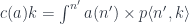
.![\mathbf{Pl}\langle s, t\rangle \langle a, b\rangle \cong \int^{c \colon [\mathcal{N}^{op} \times \mathcal{N}, Set]} [\mathcal{N}, \mathbf{Set}] \left(s, c \bullet a\right) \times [\mathcal{N}, \mathbf{Set}] \left(c \bullet b, t\right)](https://s0.wp.com/latex.php?latex=%5Cmathbf%7BPl%7D%5Clangle+s%2C+t%5Crangle+%5Clangle+a%2C+b%5Crangle+%5Ccong+%5Cint%5E%7Bc+%5Ccolon+%5B%5Cmathcal%7BN%7D%5E%7Bop%7D+%5Ctimes+%5Cmathcal%7BN%7D%2C+Set%5D%7D+++%5B%5Cmathcal%7BN%7D%2C+%5Cmathbf%7BSet%7D%5D++%5Cleft%28s%2C+c+%5Cbullet+a%5Cright%29++%5Ctimes++%5B%5Cmathcal%7BN%7D%2C+%5Cmathbf%7BSet%7D%5D++%5Cleft%28c+%5Cbullet+b%2C+t%5Cright%29+&bg=ffffff&fg=29303b&s=0&c=20201002)


![\cong \int_{n, k} \mathbf{Set}\left(c\langle k, n \rangle , [b(k), t (n)]\right)](https://s0.wp.com/latex.php?latex=%5Ccong+++%5Cint_%7Bn%2C+k%7D+%5Cmathbf%7BSet%7D%5Cleft%28c%5Clangle+k%2C+n+%5Crangle+%2C+%5Bb%28k%29%2C+t+%28n%29%5D%5Cright%29+&bg=ffffff&fg=29303b&s=0&c=20201002)
 , is:
, is:![\mathbf{Pl}\langle s, t\rangle \langle a, b\rangle \cong \int_m \mathbf{Set}\left(s(m), \int^j a(j) \times [b(j), t(m)] \right)](https://s0.wp.com/latex.php?latex=%5Cmathbf%7BPl%7D%5Clangle+s%2C+t%5Crangle+%5Clangle+a%2C+b%5Crangle+%5Ccong+%5Cint_m+%5Cmathbf%7BSet%7D%5Cleft%28s%28m%29%2C+%5Cint%5Ej+a%28j%29+%5Ctimes+%5Bb%28j%29%2C+t%28m%29%5D+%5Cright%29&bg=ffffff&fg=29303b&s=0&c=20201002)
![[\mathcal{N}, \mathbf{Set}] ( s, [b, t] \bullet a)](https://s0.wp.com/latex.php?latex=%5B%5Cmathcal%7BN%7D%2C+%5Cmathbf%7BSet%7D%5D+%28+s%2C+%5Bb%2C+t%5D+%5Cbullet+a%29&bg=ffffff&fg=29303b&s=0&c=20201002)
 of profunctors of the type:
![P \colon [\mathcal{N}, \mathbf{Set}]^{op} \times [\mathcal{N}, \mathbf{Set}] \to \mathbf{Set}](https://s0.wp.com/latex.php?latex=P+%5Ccolon+%5B%5Cmathcal%7BN%7D%2C+%5Cmathbf%7BSet%7D%5D%5E%7Bop%7D++%5Ctimes+%5B%5Cmathcal%7BN%7D%2C+%5Cmathbf%7BSet%7D%5D+%5Cto+%5Cmathbf%7BSet%7D+&bg=ffffff&fg=29303b&s=0&c=20201002)


 is the obvious forgetful functor from
 ![\mathbf{PolyLens}\langle s, t\rangle \langle a, b\rangle = \prod_{k} \mathbf{Set}\left(s_k, \sum_{n} a_n \times [b_n, t_k] \right)](https://s0.wp.com/latex.php?latex=%5Cmathbf%7BPolyLens%7D%5Clangle+s%2C+t%5Crangle+%5Clangle+a%2C+b%5Crangle+%3D+%5Cprod_%7Bk%7D+%5Cmathbf%7BSet%7D%5Cleft%28s_k%2C+%5Csum_%7Bn%7D+a_n+%5Ctimes+%5Bb_n%2C+t_k%5D+%5Cright%29+&bg=ffffff&fg=29303b&s=0&c=20201002)
 stands for a set of functions from
 ![[a, b]](https://s0.wp.com/latex.php?latex=%5Ba%2C+b%5D&bg=ffffff&fg=29303b&s=0&c=20201002) (the internal hom is the same as the external hom in
(the internal hom is the same as the external hom in  is the type of pairs
 ![\sum_{n} a_n \times [b_n, t_k]](https://s0.wp.com/latex.php?latex=%5Csum_%7Bn%7D+a_n+%5Ctimes+%5Bb_n%2C+t_k%5D+&bg=ffffff&fg=29303b&s=0&c=20201002)
 and
and  are indexed by elements of the set
  and
and  over
over 
![[t_n, y]](https://s0.wp.com/latex.php?latex=%5Bt_n%2C+y%5D&bg=ffffff&fg=29303b&s=0&c=20201002) for the internal hom:
for the internal hom:![P(y) = \sum_{n \in N} s_n \times [t_n, y]](https://s0.wp.com/latex.php?latex=P%28y%29+%3D+%5Csum_%7Bn+%5Cin+N%7D+s_n+%5Ctimes+%5Bt_n%2C+y%5D+&bg=ffffff&fg=29303b&s=0&c=20201002)
 and
and  . A natural transformation between them can be written as an end. Let’s first expand the source functor:
![\mathbf{Poly}\left( \sum_k s_k \times [t_k, -], Q\right) = \int_{y\colon \mathbf{Set}} \mathbf{Set} \left(\sum_k s_k \times [t_k, y], Q(y)\right)](https://s0.wp.com/latex.php?latex=%5Cmathbf%7BPoly%7D%5Cleft%28+%5Csum_k+s_k+%5Ctimes+%5Bt_k%2C+-%5D%2C+Q%5Cright%29++%3D++%5Cint_%7By%5Ccolon+%5Cmathbf%7BSet%7D%7D+%5Cmathbf%7BSet%7D+%5Cleft%28%5Csum_k+s_k+%5Ctimes+%5Bt_k%2C+y%5D%2C+Q%28y%29%5Cright%29&bg=ffffff&fg=29303b&s=0&c=20201002)
![\cong \prod_k \int_y \mathbf{Set} \left(s_k \times [t_k, y], Q(y)\right)](https://s0.wp.com/latex.php?latex=%5Ccong+%5Cprod_k+%5Cint_y+%5Cmathbf%7BSet%7D+%5Cleft%28s_k+%5Ctimes+%5Bt_k%2C+y%5D%2C+Q%28y%29%5Cright%29+&bg=ffffff&fg=29303b&s=0&c=20201002)
![\int_y \mathbf{Set} \left( s \times [t, y], \sum_n a_n \times [b_n, y]\right)](https://s0.wp.com/latex.php?latex=%5Cint_y+%5Cmathbf%7BSet%7D+%5Cleft%28+s+%5Ctimes+%5Bt%2C+y%5D%2C+%5Csum_n+a_n+%5Ctimes+%5Bb_n%2C+y%5D%5Cright%29+&bg=ffffff&fg=29303b&s=0&c=20201002)
![\int_y \mathbf{Set} \left( [t, y], \left[s, \sum_n a_n \times [b_n, y]\right] \right)](https://s0.wp.com/latex.php?latex=%5Cint_y+%5Cmathbf%7BSet%7D+%5Cleft%28+%5Bt%2C+y%5D%2C++%5Cleft%5Bs%2C+%5Csum_n+a_n+%5Ctimes+%5Bb_n%2C+y%5D%5Cright%5D++%5Cright%29+&bg=ffffff&fg=29303b&s=0&c=20201002)
![\int_y \mathbf{Set} \left( \mathbf{Set}(t, y), \mathbf{Set} \left(s, \sum_n a_n \times [b_n, y]\right) \right)](https://s0.wp.com/latex.php?latex=%5Cint_y+%5Cmathbf%7BSet%7D+%5Cleft%28+%5Cmathbf%7BSet%7D%28t%2C+y%29%2C+%5Cmathbf%7BSet%7D+%5Cleft%28s%2C+%5Csum_n+a_n+%5Ctimes+%5Bb_n%2C+y%5D%5Cright%29++%5Cright%29+&bg=ffffff&fg=29303b&s=0&c=20201002)
 with
with ![\mathbf{Set}\left(s, \sum_n a_n \times [b_n, t] \right)](https://s0.wp.com/latex.php?latex=%5Cmathbf%7BSet%7D%5Cleft%28s%2C+%5Csum_n+a_n+%5Ctimes+%5Bb_n%2C+t%5D+%5Cright%29+&bg=ffffff&fg=29303b&s=0&c=20201002)
![\sum_k s_k \times [t_k, y]](https://s0.wp.com/latex.php?latex=%5Csum_k+s_k+%5Ctimes+%5Bt_k%2C+y%5D&bg=ffffff&fg=29303b&s=0&c=20201002) and
and ![\sum_n a_n \times [b_n, y]](https://s0.wp.com/latex.php?latex=%5Csum_n+a_n+%5Ctimes+%5Bb_n%2C+y%5D&bg=ffffff&fg=29303b&s=0&c=20201002) is called a polynomial lens. Combining the previous results, we see that it can be written as:
is called a polynomial lens. Combining the previous results, we see that it can be written as:![\mathbf{PolyLens}\langle s, t\rangle \langle a, b\rangle = \prod_{k \in K} \mathbf{Set}\left(s_k, \sum_{n \in N} a_n \times [b_n, t_k] \right)](https://s0.wp.com/latex.php?latex=%5Cmathbf%7BPolyLens%7D%5Clangle+s%2C+t%5Crangle+%5Clangle+a%2C+b%5Crangle+%3D+%5Cprod_%7Bk+%5Cin+K%7D+%5Cmathbf%7BSet%7D%5Cleft%28s_k%2C+%5Csum_%7Bn+%5Cin+N%7D+a_n+%5Ctimes+%5Bb_n%2C+t_k%5D+%5Cright%29+&bg=ffffff&fg=29303b&s=0&c=20201002)
 depends not only on the type but also on the value of the argument
  .
.![Lan_b a \cong \int^{n \colon \mathcal{N}} a \times [b, -]](https://s0.wp.com/latex.php?latex=Lan_b+a+%5Ccong+%5Cint%5E%7Bn+%5Ccolon+%5Cmathcal%7BN%7D%7D+a+%5Ctimes+%5Bb%2C+-%5D+&bg=ffffff&fg=29303b&s=0&c=20201002)
 becomes a product. An end of hom-sets becomes a natural transformation. A polynomial lens can therefore be rewritten as:
![\prod_{k \in K} \mathbf{Set}\left(s_k, \sum_{n \in N} a_n \times [b_n, t_k] \right) \cong [\mathcal{K}, \mathbf{Set}](s, (Lan_b a) \circ t)](https://s0.wp.com/latex.php?latex=%5Cprod_%7Bk+%5Cin+K%7D+%5Cmathbf%7BSet%7D%5Cleft%28s_k%2C+%5Csum_%7Bn+%5Cin+N%7D+a_n+%5Ctimes+%5Bb_n%2C+t_k%5D+%5Cright%29++%5Ccong+%5B%5Cmathcal%7BK%7D%2C+%5Cmathbf%7BSet%7D%5D%28s%2C+%28Lan_b+a%29+%5Ccirc+t%29+&bg=ffffff&fg=29303b&s=0&c=20201002)
](https://s0.wp.com/latex.php?latex=%5Cmathbf%7BPolyLens%7D%5Clangle+s%2C+t%5Crangle+%5Clangle+a%2C+b%5Crangle+%5Ccong+%5B%5Cmathbf%7BSet%7D%2C+%5Cmathbf%7BSet%7D%5D%28Lan_t+s%2C+Lan_b+a%29+&bg=ffffff&fg=29303b&s=0&c=20201002)

![\prod_{i \in K} \prod_{m \in N} \mathbf{Set}\left(c_{m i}, [b_m, t_i ]\right)](https://s0.wp.com/latex.php?latex=%5Cprod_%7Bi+%5Cin+K%7D+%5Cprod_%7Bm+%5Cin+N%7D+%5Cmathbf%7BSet%7D%5Cleft%28c_%7Bm+i%7D%2C+%5Bb_m%2C+t_i+%5D%5Cright%29&bg=ffffff&fg=29303b&s=0&c=20201002)
![\prod_{i \in K} \prod_{m \in N} \mathbf{Set} \left(c_{m i}, [b_m, t_i] \right) \cong [\mathcal{N}^{op} \times \mathcal{K}, \mathbf{Set}]\left(c_{= -}, [b_=, t_- ]\right)](https://s0.wp.com/latex.php?latex=%5Cprod_%7Bi+%5Cin+K%7D+%5Cprod_%7Bm+%5Cin+N%7D+%5Cmathbf%7BSet%7D+%5Cleft%28c_%7Bm+i%7D%2C+%5Bb_m%2C+t_i%5D+%5Cright%29+%5Ccong+%5B%5Cmathcal%7BN%7D%5E%7Bop%7D+%5Ctimes+%5Cmathcal%7BK%7D%2C+%5Cmathbf%7BSet%7D%5D%5Cleft%28c_%7B%3D+-%7D%2C+%5Bb_%3D%2C+t_-+%5D%5Cright%29&bg=ffffff&fg=29303b&s=0&c=20201002)
 .
. . The result is that
  can be wrtitten as:
![\int^{c_{k i}} \prod_{k \in K} \mathbf{Set} \left(s_k, \sum_{n \in N} a_n \times c_{n k} \right) \times [\mathcal{N}^{op} \times \mathcal{K}, \mathbf{Set}]\left(c_{= -}, [b_=, t_- ]\right)](https://s0.wp.com/latex.php?latex=%5Cint%5E%7Bc_%7Bk+i%7D%7D+%5Cprod_%7Bk+%5Cin+K%7D+%5Cmathbf%7BSet%7D+%5Cleft%28s_k%2C++%5Csum_%7Bn+%5Cin+N%7D+a_n+%5Ctimes+c_%7Bn+k%7D+%5Cright%29+%5Ctimes+%5B%5Cmathcal%7BN%7D%5E%7Bop%7D+%5Ctimes+%5Cmathcal%7BK%7D%2C+%5Cmathbf%7BSet%7D%5D%5Cleft%28c_%7B%3D+-%7D%2C+%5Bb_%3D%2C+t_-+%5D%5Cright%29+&bg=ffffff&fg=29303b&s=0&c=20201002)
![\cong \prod_{k \in K} \mathbf{Set}\left(s_k, \sum_{n \in N} a_n \times [b_n, t_k] \right)](https://s0.wp.com/latex.php?latex=%5Ccong++%5Cprod_%7Bk+%5Cin+K%7D+%5Cmathbf%7BSet%7D%5Cleft%28s_k%2C+%5Csum_%7Bn+%5Cin+N%7D+a_n+%5Ctimes+%5Bb_n%2C+t_k%5D+%5Cright%29+&bg=ffffff&fg=29303b&s=0&c=20201002)
 :
:
![\mathcal{C}(c \times b, t) \cong \mathcal{C}(c, [b, t])](https://s0.wp.com/latex.php?latex=%5Cmathcal%7BC%7D%28c+%5Ctimes+b%2C+t%29+%5Ccong++%5Cmathcal%7BC%7D%28c%2C+%5Bb%2C+t%5D%29+&bg=ffffff&fg=29303b&s=0&c=20201002)
![[b, t]](https://s0.wp.com/latex.php?latex=%5Bb%2C+t%5D&bg=ffffff&fg=29303b&s=0&c=20201002) is the internal hom, or the function object
is the internal hom, or the function object 
 from the category
 ![\mathcal{L}\langle s, t\rangle \langle a, b \rangle \cong \int^{c} \mathcal{C}(s, c \times a) \times \mathcal{C}(c, [b, t]) \cong \mathcal{C}(s, [b, t] \times a)](https://s0.wp.com/latex.php?latex=%5Cmathcal%7BL%7D%5Clangle+s%2C+t%5Crangle+%5Clangle+a%2C+b+%5Crangle+%5Ccong+%5Cint%5E%7Bc%7D+%5Cmathcal%7BC%7D%28s%2C+c+%5Ctimes+a%29+%5Ctimes++%5Cmathcal%7BC%7D%28c%2C+%5Bb%2C+t%5D%29+%5Ccong+%5Cmathcal%7BC%7D%28s%2C+%5Bb%2C+t%5D+%5Ctimes+a%29+&bg=ffffff&fg=29303b&s=0&c=20201002)
![\mathcal{C}(s, [b, t]) \times \mathcal{C}(s, a)](https://s0.wp.com/latex.php?latex=%5Cmathcal%7BC%7D%28s%2C+%5Bb%2C+t%5D%29+%5Ctimes+%5Cmathcal%7BC%7D%28s%2C+a%29+&bg=ffffff&fg=29303b&s=0&c=20201002)

 is monoidal, and it has an action defiend on both
  . A category with a monoidal action is called an actegory.
 ).
).
 in
in 


 , and use the mapping:
![L \colon \mathcal{M} \to [\mathcal{C}, \mathcal{C}]](https://s0.wp.com/latex.php?latex=L+%5Ccolon+%5Cmathcal%7BM%7D+%5Cto+%5B%5Cmathcal%7BC%7D%2C+%5Cmathcal%7BC%7D%5D+&bg=ffffff&fg=29303b&s=0&c=20201002)
![[\mathcal{C}, \mathcal{C}]](https://s0.wp.com/latex.php?latex=%5B%5Cmathcal%7BC%7D%2C+%5Cmathcal%7BC%7D%5D&bg=ffffff&fg=29303b&s=0&c=20201002) , which is naturally equipped with a monoidal structure given by functor composition (and, as we well know, a monad is just a monoid in that category).
, which is naturally equipped with a monoidal structure given by functor composition (and, as we well know, a monad is just a monoid in that category). be a strict monoidal functor, mapping tensor product to functor composition and unit object to identity functor.


 . In that case we have:
 is an object in
 is covariant in
 , we can define the hom-object as:


 in an enriched category must satisfy the composition and identity laws. In an enriched category, composition is a mapping:
 . We get:

 .
.
 .
. is automatically self-enriched. The copower action
  is equivalent to enrichment over
  .
.

 by injecting a pair of morphisms from the two hom-sets sharing the same
 ![\mathcal{C}(c \times b, t) \cong \mathcal{C}(c, [b, t])](https://s0.wp.com/latex.php?latex=%5Cmathcal%7BC%7D%28c+%5Ctimes+b%2C+t%29+%5Ccong+%5Cmathcal%7BC%7D%28c%2C+%5Bb%2C+t%5D%29&bg=ffffff&fg=29303b&s=0&c=20201002)
![\int^{c : \mathcal{C}} \mathcal{C}(s, c \times a) \times \mathcal{C}(c, [b, t]) \cong \mathcal{C}(s, [b, t] \times a) \cong \mathcal{C}(s \times b, t) \times \mathcal{C}(s, a)](https://s0.wp.com/latex.php?latex=%5Cint%5E%7Bc+%3A+%5Cmathcal%7BC%7D%7D+%5Cmathcal%7BC%7D%28s%2C+c+%5Ctimes+a%29+%5Ctimes+%5Cmathcal%7BC%7D%28c%2C+%5Bb%2C+t%5D%29+%5Ccong+%5Cmathcal%7BC%7D%28s%2C+%5Bb%2C+t%5D+%5Ctimes+a%29+%5Ccong+%5Cmathcal%7BC%7D%28s+%5Ctimes+b%2C+t%29+%5Ctimes+%5Cmathcal%7BC%7D%28s%2C+a%29&bg=ffffff&fg=29303b&s=0&c=20201002)


 , and further decompose
  , then you can decompose
  . Zooming-in is made possible by the associativity of the tensor product.
 to
to  is the optic
  . Zooming-in is the composition of morphisms.
 in
in 

 is the unit object with respect to the tensor product
  is the identity endofunctor.)
 .
. in
in  in
in 
 . It’s a cross between a coproduct and a trace, as it’s constructed using injections of diagonal elements (with some identifications):
 :
:
 , the base space
  , and a projection, or a display map,
  . The fibers of
  (a free monoid generated by
  ) with the projection
  that returns the length of a list.
 . Counted vectors, for instance, are represented as objects in
  given by pairs
  . Morphisms in the slice category correspond to fibre-wise mappings between bundles.
 has both the left adjoint, the dependent sum
  ; and the right adjoint, the dependent product
  . The base-change functor is defined as a pullback:
 and
and  . In a locally cartesian closed category, this product has the right adjoint, the internal hom in
 .
.


 are objects in the appropriate slice categories.
 on another object
  is given by the pullback:

![\cong \int^{\langle C, p \rangle : \mathcal{C}/B} (\mathcal{C}/B)( S, C \times_B A) \times (\mathcal{C}/B)(C , [A', S']_B)](https://s0.wp.com/latex.php?latex=%5Ccong+%5Cint%5E%7B%5Clangle+C%2C+p+%5Crangle+%3A+%5Cmathcal%7BC%7D%2FB%7D+%28%5Cmathcal%7BC%7D%2FB%29%28+S%2C+C+%5Ctimes_B+A%29+%5Ctimes+%28%5Cmathcal%7BC%7D%2FB%29%28C+%2C+%5BA%27%2C+S%27%5D_B%29+&bg=ffffff&fg=29303b&s=0&c=20201002)
![(\mathcal{C}/B)( S, [A', S']_B \times_B A)](https://s0.wp.com/latex.php?latex=%28%5Cmathcal%7BC%7D%2FB%29%28+S%2C+%5BA%27%2C+S%27%5D_B+%5Ctimes_B+A%29+&bg=ffffff&fg=29303b&s=0&c=20201002)
![[A', S']_B](https://s0.wp.com/latex.php?latex=%5BA%27%2C+S%27%5D_B&bg=ffffff&fg=29303b&s=0&c=20201002) in a locally cartesian closed category can be expressed using a dependent product:
in a locally cartesian closed category can be expressed using a dependent product:![\left [\left \langle A' \atop p \right \rangle, \left \langle S' \atop q \right \rangle \right ] \cong \Pi_p \left(p^* \left \langle S' \atop q \right \rangle \right)](https://s0.wp.com/latex.php?latex=%5Cleft+%5B%5Cleft+%5Clangle+A%27+%5Catop+p+%5Cright+%5Crangle%2C+%5Cleft+%5Clangle+S%27+%5Catop+q+%5Cright+%5Crangle+%5Cright+%5D+%5Ccong+%5CPi_p+%5Cleft%28p%5E%2A+%5Cleft+%5Clangle+S%27+%5Catop+q+%5Cright+%5Crangle+%5Cright%29&bg=ffffff&fg=29303b&s=0&c=20201002)
 is the fibration of
  is the right adjoint to the base change functor, and
  is the base-change functor along
 , this is equal to an infinite tuple of functions:
 indexed by
 can be expressed as a fibration
  , with
  , the sum of the fibers. The set of powers of
  , with
  the type of list of
  the function that assigns the length to a list. The monoidal action can then be written using a product (pullback) in the slice category
  :
:
 , which can be used to express the polynomial action:


 is the projection from the cartesian product.
![(\mathbf{Set}/\mathbb{N})\left(\left \langle {C \atop p} \right \rangle, \left[ \left \langle {L(b) \atop \mathit{len}} \right \rangle, \left \langle {\mathbb{N} \times t \atop \pi_1} \right \rangle \right] \right)](https://s0.wp.com/latex.php?latex=%28%5Cmathbf%7BSet%7D%2F%5Cmathbb%7BN%7D%29%5Cleft%28%5Cleft+%5Clangle+%7BC+%5Catop+p%7D+%5Cright+%5Crangle%2C+%5Cleft%5B+%5Cleft+%5Clangle+%7BL%28b%29+%5Catop+%5Cmathit%7Blen%7D%7D+%5Cright+%5Crangle%2C+%5Cleft+%5Clangle+%7B%5Cmathbb%7BN%7D+%5Ctimes+t+%5Catop+%5Cpi_1%7D+%5Cright+%5Crangle+%5Cright%5D+%5Cright%29+&bg=ffffff&fg=29303b&s=0&c=20201002)
 and get:
![O(a, b; s, t) \cong \mathbf{Set} \left( s, U\left( \left[ \left \langle {L(b) \atop \mathit{len}} \right \rangle, \left \langle {\mathbb{N} \times t \atop \pi_1} \right \rangle \right] \times \left \langle {L(a) \atop \mathit{len}} \right \rangle \right) \right)](https://s0.wp.com/latex.php?latex=O%28a%2C+b%3B+s%2C+t%29+%5Ccong+%5Cmathbf%7BSet%7D+%5Cleft%28+s%2C+U%5Cleft%28+%5Cleft%5B+%5Cleft+%5Clangle+%7BL%28b%29+%5Catop+%5Cmathit%7Blen%7D%7D+%5Cright+%5Crangle%2C+%5Cleft+%5Clangle+%7B%5Cmathbb%7BN%7D+%5Ctimes+t+%5Catop+%5Cpi_1%7D+%5Cright+%5Crangle+%5Cright%5D+%5Ctimes+%5Cleft+%5Clangle+%7BL%28a%29+%5Catop+%5Cmathit%7Blen%7D%7D+%5Cright+%5Crangle+%5Cright%29+%5Cright%29+&bg=ffffff&fg=29303b&s=0&c=20201002)


