A lens is a reification of the concept of object composition. In a nutshell, it describes the process of decomposing the source object into a focus and a residue and recomposing a new object from a new focus and the same residue .
The key observation is that we don’t care what the residue is as long as it exists. This is why a lens can be implemented, in Haskell, as an existential type:
data Lens s t a b where
 Lens :: (s -> (c, a)) -> ((c, b) -> t) -> Lens s t a b
In category theory, the existential type is represented as a coend—essentially a gigantic sum over all objects in the category :
There is a simple recipe to turn this representation into the more familiar one. The first step is to use the currying adjunction on the second hom-functor:
Here, is the internal hom, or the function object (b->t).
Once the object appears as the source in the hom-set, we can use the co-Yoneda lemma to eliminate the coend. This is the formula we use:
It works for any functor from the category to so, in particular we have:
The result is a pair of arrows:
the first corrsponding to:
set :: s -> b -> t
and the second to:
get :: s -> a
It turns out that this trick works for more general optics. It all depends on being able to isolate the object as the source of the second hom-set.
We’ve been able to do it case-by-case for lenses, prisms, traversals, and the whole zoo of optics. It turns out that the same problem was studied in all its generality by Australian category theorists Janelidze and Kelly in a context that had nothing to do with optics.
Monoidal Actions
Here’s the most general definition of an optic:
This definition involves three separate categories. The category is monoidal, and it has an action defiend on both and . A category with a monoidal action is called an actegory.
We get the definition of a lens by having all three categories be the same—a cartesian closed category . We define the action of this category on itself:
(and the same for ).
There are two equivalent ways of defining the action of a monoidal category. One is as the mapping
written in infix notation as . It has to be equipped with two additional structure maps—isomorphisms that relate the tensor product in and its unit to the action in :
plus some coherence conditions corresponding to associativity and unit laws.
Using this notation, we can rewrite the definition of an optic as:
with the understanding that we use the same symbol for two different actions in and .
Alternatively, we can curry the action , and use the mapping:
The target category here is the category of endofunctors , which is naturally equipped with a monoidal structure given by functor composition (and, as we well know, a monad is just a monoid in that category).
The two structure maps from the definition of translate to the requirement that be a strict monoidal functor, mapping tensor product to functor composition and unit object to identity functor.
The Adjunction
When we were eliminating the coend in the definition of a lens, we used the currying adjunction. This particular adjunction works inside a single category but, in general, an adjunction relates two functors between a pair of categories. Therefore, to eliminate the end from the optic, we need an adjunction that looks like this:
The category on the right is the monoidal category , because is the object from this category.
Using the adjunction and the co-Yoneda lemma we get:
There is a whole slew of monoidal actions that have the right adjoint of this type. Let’s look at an example.
The category of sets is a monoidal category, and we can define its action on another category using the formula:
This is the definition of a copower. A category in which this adjunction holds for all objects is called copowered or tensored over .
The intuition is that a copower is like an iterated sum (hence the multiplication sign). Indeed, a mapping out of a coproduct of copies of , where is a set, is equivalent to mappings out of .
This formula generalizes to the case in which is a category enriched over a monoidal category . In that case we have:
Here, the hom is an object in .
Relation to Enrichment
We are interested in the adjunction:
The functor is covariant in and contravariant in :
In other words, it’s a profunctor. In fact, it has the right signature to be a hom-functor. And this is what Janelidze and Kelly show: the functor can serve as the hom-functor that generates the enrichment for . If we call the enriched category , we can define the hom-object as:
Our adjunction can be rewritten as:
The counit of this adjunction is a mapping:
which is analogous to function application.
The hom-object in an enriched category must satisfy the composition and identity laws. In an enriched category, composition is a mapping:
Let’s see if we can get this mapping from our adjunction by replacing with . We get:
The right-hand side should contain the mapping we’re looking for. All we need is to point at a morphism on the left. Indeed, we can define it as the following composite:
We used the structure map and (twice) the counit of the adjunction .
Similarly, the identity of composition, which is the mapping:
is adjoint to the other structure map .
Janelidze and Kelly go on to prove that the action of a monoidal right-closed category having the right adjoint is equivalent to the existence of the tensored enrichment of the category on which this action is defined.
The two examples of monoidal actions we’ve seen so far are indeed equivalent to enrichments. A cartesian closed category in which we defined the action is automatically self-enriched. The copower action is equivalent to enrichment over (which doesn’t mean much, since regular categories are naturally -enriched; but not all of them are tensored).
Acknowledgments
I’m grateful to Jules Hedges and his collaborators for sharing their insights and unpublished notes with me.
Category theory extracts the essence of structure and composition. At its foundation it deals with the composition of arrows. Building on composition of arrows it then goes on describing the ways objects can be composed: we have products, coproducts and, at a higher level, tensor products. They all describe various modes of composing objects. In monoidal categories any two objects can be composed.
Unlike composition, which can be described uniformly, decomposition requires case-by-case treatment. It’s easy to decompose a cartesian product using projections. A coproduct (sum) can be decomposed using pattern matching. A generic tensor product, on the other hand, has no standard means of decompositon.
Optics is the essence of decomposition. It answers the question of what it means to decompose a composite.
We consider an object decomposable when:
We can split it into the focus and the complement,
We can replace the focus with something else, without changing the complement, to get a new composite object,
We can zoom in; that is, if the focus is decomposable, we can compose the two decompositions,
It’s possible for the whole object to be the focus.
Let’s translate these requirements into the language of category theory. We’ll start with the standard example: the lens, which is the optic for decomposing cartesian products.
The splitting means that there is a morphism from the composite object to the product , where is the complement and is the focus. This morphism is a member of the hom-set .
To replace the focus we need another morphism that takes the same complement , combines it with the new focus to produce the new composite . This morphism is a member of the hom-set
Here’s the important observation: We don’t care what the complement is. We are “focusing” on the focus. We carry the complement over to combine it with the new focus, but we don’t use it for anything else. It’s a featureless black box.
To erase the identity of the complement, we hide it inside a coend. A coend is a generalization of a sum, so it is written using the integral sign (see the Appendix for details). Programmers know it as an existential type, logicians call it an existential quantifier. We say that there exists a complement , but we don’t care what it is. We “integrate” over all possible complements.
Here’s the existential definition of the lens:
Just like we construct a coproduct using one of the injections, so the coend is constructed using one of (possibly infinite number of) injections. In our case we construct a lens by injecting a pair of morphisms from the two hom-sets sharing the same . But once the lens is constructed, there is no way to extract the original from it.
It’s not immediately obvious that this representation of the lens reproduces the standard setter/getter form. However, in a cartesian closed category, we can use the currying adjunction to transform the second hom-set:
Here, is the internal hom, or the function object representing morphisms from to . We can then use the co-Yoneda lemma to reduce the coend:
The first part of this product is the setter: it takes the source object and the new focus to produce the new target . The second part is the getter that extracts the focus .
Even though all optics have similar form, each of them reduces differently.
Here’s another example: the prism. We just replace the product with the coproduct (sum).
This time the reduction goes through the universal property of the coproduct: a mapping out of a sum is a product of mappings:
Again, we use the co-Yoneda to reduce the coend:
The first one extracts the focus , if possible, otherwise it constructs a (by secretly injecting a ). The second constructs a by injecting a .
We can easily generalize existential optics to an arbitrary tensor product in a monoidal category:
In general, though, this form cannot be further reduced using the co-Yoneda trick.
But what about the third requirement: the zooming-in property of optics? In the case of the lens and the prism it works because of associativity of the product and the sum. In fact it works for any tensor product. If you can decompose into , and further decompose into , then you can decompose into . Zooming-in is made possible by the associativity of the tensor product.
Focusing on the whole object plays the role of the unit of zooming.
These two properties are used in the definition of the category of optics. The objects in this category are pairs of object in . A morphism from a pair to is the optic . Zooming-in is the composition of morphisms.
But this is still not the most general setting. The useful insight is that the multiplication (product) in a lens, and addition (coproduct) in a prism, look like examples of linear transformations, with the residue playing the role of a parameter. In fact, a composition of a lens with a prism produces a 2-parameter affine transformation, which also behaves like an optic. We can therefore generalize optics to work with an arbitrary monoidal action (first hinted in the discussion at the end of this blog post). Categories with such actions are known as actegories.
The idea is that you define a family of endofunctors in that is parameterized by objects from a monoidal category . So far we’ve only discussed examples where the parameters were taken from the same category and the action was either multiplication or addition. But there are many examples in which is not the same as .
The zooming principles are satisfied if the action respects the tensor product in :
(Here, is the unit object with respect to the tensor product in , and is the identity endofunctor.)
The actegorical version of the optic doesn’t deal directly with the residue. It tells us that the “unimportant” part of the composite object can be parameterized by some .
This additional abstraction allows us to transport the residue between categories. It’s enough that we have one action in and another in to create this mixed optics (first introduced by Mitchell Riley):
The separation of the focus from the complement using monoidal actions is reminiscent of what physicists call the distinction between “physical” and “gauge” degrees of freedom.
An in-depth presentation of optics, including their profunctor representation, is available in this paper.
Appendix: Coends and the Co-Yoneda Lemma
A coend is defined for a profunctor, that is a functor of two variables, one contravariant and one covariant, . It’s a cross between a coproduct and a trace, as it’s constructed using injections of diagonal elements (with some identifications):
Co-Yoneda lemma is the identity that works for any covariant functor (copresheaf) :
A PDF version of this post is available on GitHub.
Dependent types, in programming, are families of types indexed by elements of an indexing type. For instance, counted vectors are families of tuples indexed by natural numbers—the lengths of the vectors.
In category theory we model dependent types as fibrations. We start with the total space , the base space , and a projection, or a display map, . The fibers of correspond to members of the type family. For instance, the total space, or the bundle, of counted vectors is the list type (a free monoid generated by ) with the projection that returns the length of a list.
Another way of looking at dependent types is as objects in the slice category . Counted vectors, for instance, are represented as objects in given by pairs . Morphisms in the slice category correspond to fibre-wise mappings between bundles.
We often require that be a locally cartesian closed category, that is a category whose slice categories are cartesian closed. In such categories, the base-change functor has both the left adjoint, the dependent sum ; and the right adjoint, the dependent product . The base-change functor is defined as a pullback:
This pullback defines a cartesian product in the slice category between two objects: and . In a locally cartesian closed category, this product has the right adjoint, the internal hom in .
Dependent optics
The most general optic is given by two monoidal actions and in two categories and . It can be written as the following coend of the product of two hom-sets:
Monoidal actions are parameterized by objects in a monoidal category .
Dependent optics are a special case of general optics, where one or both categories in question are slice categories. When the monoidal action is defined in the slice category, the transformations must respect fibrations. For instance, the action in the bundle over must commute with the projection:
This is reminiscent of gauge transformations in physics, which act on fibers in bundles over spacetime. The action must respect the monoidal structure of so, for instance,
We can define a dependent (mixed) optic as:
Just like regular optics, dependent optics can be represented using Tambara modules, which are profunctors with the additional structure given by transformations:
where and are objects in the appropriate slice categories.
The optic is then given by the following end in the Tambara category:
Dependent lens
The primordial optic, the lens, is defined by the monoidal action of a product. By analogy, we define a dependent lens by the action of the product in a slice category. The action parameterized by an object on another object is given by the pullback:
Since a pullback is the product in the slice category , it is automatically associative and unital, so it can be used to define a dependent lens:
Since is locally cartesian closed, there is an adjunction between the product and the exponential. We can use it to get:
We can then apply the Yoneda lemma to get the setter/getter form:
The internal hom in a locally cartesian closed category can be expressed using a dependent product:
where is the fibration of , is the right adjoint to the base change functor, and is the base-change functor along .
The dependent lens can be written as:
In particular, if is , this is equal to an infinite tuple of functions:
or fiber-wise pairs of setter/getter indexed by .
Traversals
Traversals are optics whose monoidal action is generated by polynomial functors of the form:
The coefficients can be expressed as a fibration , with , the sum of the fibers. The set of powers of can be similarly written as , with the type of list of (a free monoid generated by ), and the function that assigns the length to a list. The monoidal action can then be written using a product (pullback) in the slice category :
There is an obvious forgetful functor , which can be used to express the polynomial action:
The traversal is the optic:
Eqivalently, the second factor can be rewritten as:
This, in turn, is equivalent to a single hom-set in the slice category:
where is the projection from the cartesian product.
The traversal is therefore a mixed optic:
The second factor can be transformed using the internal hom adjunction:
We can then use the ninja Yoneda lemma on the optic to “integrate” over and get:
A traversal is a kind of optic that can focus on zero or more items at a time. Naively, we would expect to have a getter that returns a list of values, and a setter that replaces a list of values. Think of a tree with leaves: a traversal would return a list of leaves, and it would allow you to replace them with a new list. The problem is that the size of the list you pass to the setter cannot be arbitrary—it must match the number of leaves in the particular tree. This is why, in Haskell, the setter and the getter are usually combined in a single function:
s -> ([b] -> t, [a])
Still, Haskell is not able to force the sizes of both lists to be equal.
Since a list type can be represented as an infinite sum of tuples, I knew that the categorical version of this formula must involve a power series, or a polynomial functor:
but was unable to come up with an existential form for it.
Pickering, Gibbons, and Wu came up with a representation for traversals using profunctors that were cartesian, cocartesian, and monoidal at the same time, but the monoidal constraint didn’t fit neatly into the Tambara scheme:
class Profunctor p => Monoidal p where
  par   :: p a b -> p c d -> p (a, c) (b, d)
  empty :: p () ()
We’ve been struggling with this problem, when one of my students, Mario Román came up with the ingenious idea to make existential.
The idea is that a coend in the existential representation of optics acts like a sum (or like an integral—hence the notation). A sum over natural numbers is equivalent to the coend over the category of natural numbers.
At the root of all optics there is a monoidal action. For lenses, this action is given by “scaling”
For prisms, it’s the “translation”
For grates it’s the exponentiation
The composition of a prism and a lens is an affine transformation
A traversal is similarly generated by a polynomial functor, or a power series functor:
The key observation here is that there is a different object for every power of , which can only be expressed using dependent types in programming. For every multiplicity of foci, the residue is of a different type.
In category theory, we can express the whole infinite sequence of residues as a functor from the monoidal category of natural numbers to . (The sum is really a coend over .)
The existential version of a traversal is thus given by:
We can now use the continuity of the hom-set to replace the mapping out of a sum with a product of mappings:
and use the currying adjunction
The product of hom-sets is really an end over , or a set of natural transformations in
and we can apply the Yoneda lemma to “integrate” over to get:
which is exactly the formula for traversals.
Once we understood the existential representation of traversals, the profunctor representation followed. The equivalent of Tambara modules for traversals is a category of profunctors equipped with the monoidal action parameterized by objects in :
The double Yoneda trick works for these profunctors as well, proving the equivalence with the existential representation.
Generalizations
As hinted in my blog post and formalized by Mitchell Riley, Tambara modules can be generalized to an arbitrary monoidal action. We have also realized that we can combine actions in two different categories. We could take an arbitrary monoidal category , define its action on two categories, and using strong monoidal functors:
These actions define the most general existential optic:
Notice that the pairs of arguments are heterogenous—e.g., in , is from , and is from .
We have also generalized Tambara modules:
and the Pastro Street derivation of the promonad. That lead us to a more general proof of isomorphism between the profunctor formulation and the existential formulation of optics. Just to be general enough, we did it for enriched categories, replacing with an arbitrary monoidal category.
Finally, we described some new interesting optics like algebraic and monadic lenses.
The Physicist’s Explanation
The traversal result confirmed my initial intuition from general relativity that the most general optics are generated by the analog of diffeomorphisms. These are the smooth coordinate transformations under which Einstein’s theory is covariant.
Physicists have long been using symmetry groups to build theories. Laws of physics are symmetric with respect to translations, time shifts, rotations, etc.; leading to laws of conservation of momentum, energy, angular momentum, etc. There is an uncanny resemblance of these transformations to some of the monoidal actions in optics. The prism is related to translations, the lens to rotations or scaling, etc.
There are many global symmetries in physics, but the real power comes from local symmetries: gauge symmetries and diffeomorphisms. These give rise to the Standard Model and to Einstein’s theory of gravity.
A general monoidal action seen in optics is highly reminiscent of a diffeomorphism, and the symmetry behind a traversal looks like it’s generated by an analytical function.
In my opinion, these similarities are a reflection of a deeper principle of compositionality. There is only a limited set of ways we can decompose complex problems, and sooner or later they all end up in category theory.
The main difference between physics and category theory is that category theory is more interested in one-way mappings, whereas physics deals with invertible transformations. For instance, in category theory, monoids are more fundamental than groups.
Here’s how categorical optics might be seen by a physicist.
In physics we would start with a group of transformations. Its representations would be used, for instance, to classify elementary particles. In optics we start with a monoidal category and define its action in the target category . (Notice the use of a monoid rather than a group.)
In physics we would represent the group using matrices, here we use endofunctors.
A profunctor is like a path that connects the initial state to the final state. It describes all the ways in which can evolve into .
If we use mixed optics, final states come from a different category , but their transformations are parameterized by the same monoidal category:
A path may be arbitrarily extended, at both ends, by a pair of morphisms. Given a morphism in :
and another one in
the profunctor uses them to extend the path:
A (generalized) Tambara module is like the space of paths that can be extended by transforming their endpoints.
If we have a path that can evolve into , then the same path can be used to evolve into . In physics, we would say that the paths are “invariant” under the transformation, but in category theory we are fine with a one-way mapping.
The profunctor representation is like a path integral:
We fix the end-states but we vary the paths. We integrate over all paths that have the “invariance” or extensibility property that defines the Tambara module.
For every such path, we have a mapping that takes the evolution from to and produces the evolution (along the same path) from to .
The main theorem of profunctor optics states that if, for a given collection of states, , such a mapping exists, then these states are related. There exists a transformation and a pair of morphisms that are secretly used in the path integral to extend the original path.
Again, the mappings are one-way rather than both ways. They let us get from to and from to .
This pair of morphisms is enough to extend any path to by first applying and then lifting the two morphisms. The converse is also true: if every path can be extended then such a pair of morphisms must exist.
What seems unique to optics is the interplay between transformations and decompositions: The way can be interpreted both as parameterizing a monoidal action and the residue left over after removing the focus.
Conclusion
For all the details and a list of references you can look at our paper “Profunctor optics, a categorical update.” It’s the result of our work at the Adjoint School of Applied Category Theory in Oxford in 2019. It’s avaliable on arXiv.
I’d like to thank Mario Román for reading the draft and providing valuable feedback.
could be interpreted as the representable functor acting as the unit with respect to taking the end. It takes an and returns an . Let’s keep this in mind.
We are going to need an identity that involves higher-order natural transformations between two higher-order functors. These are actually the functors that we’ve encountered before. They are parameterized by objects in , and their action on functors (co-presheaves) is to apply those functors to objects. They are the “give me a functor and I’ll apply it to my favorite object” kind of functors.
We need a natural transformation between two such functors, and we can express it as an end:
Here’s the trick: replace these functors with their Yoneda equivalents:
Notice that this is now a mapping between two hom-sets in the functor category, the first one being:
We can now use the corollary of the Yoneda lemma to replace the set of natural transformation between these two hom-functors with the hom-set:
But this is again a natural transformation between two hom-functors, so it can be further reduced to . The result is:
We’ve used the Yoneda lemma twice, so this trick is called the double-Yoneda.
Profunctors
It turns out that the prism also has a functor-polymorphic representation, but it uses profunctors in place of regular functors. A profunctor is a functor of two arguments, but its action on arrows has a twist. Here’s the Haskell definition:
class Profunctor p where
  dimap :: (a' -> a) -> (b -> b') -> (p a b -> p a' b')
It lifts a pair of functions, where the first one goes in the opposite direction.
In category theory, the “twist” is encoded by using the opposite category , so a profunctor is defined a functor from to .
The prime example of a profunctor is the hom-functor which, on objects, assigns the set to every pair .
Before we talk about the profunctor representation of prisms and lenses, there is a simple optic called Iso. It’s defined by a pair of functions:
from :: s -> a
to   :: b -> t
The key observation here is that such a pair of arrows is an element of the hom set in the category between the pair and the pair :
The “twist” of using reverses the direction of the first arrow.
Iso has a simple profunctor representation:
type Iso s t a b = forall p. Profunctor p => p a b -> p s t
This formula can be translated to category theory as an end in the profunctor category:
Profunctor category is a category of co-presheaves . We can immediately apply the double Yoneda identity to it to get:
which shows the equivalence of the two representations.
Tambara Modules
Here’s the profunctor representation of a prism:
type Prism s t a b = forall p. Choice p => p a b -> p s t
It looks almost the same as Iso, except that the quantification goes over a smaller class of profunctors called Choice (or cocartesian). This class is defined as:
class Profunctor p => Choice where
  left'  :: p a b -> p (Either a c) (Either b c)
  right' :: p a b -> p (Either c a) (Either c b)
Lenses can also be defined in a similar way, using the class of profunctors called Strong (or cartesian).
class Profunctor p => Strong where
  first'  :: p a b -> p (a, c) (b, c)
  second' :: p a b -> p (c, a) (c, b)
Profunctor categories with these structures are called Tambara modules. Tambara formulated them in the context of monoidal categories, for a more general tensor product. Sum (Either) and product (,) are just two special cases.
A Tambara module is an object in a profunctor category with additional structure defined by a family of morphisms:
with some naturality and coherence conditions.
Lenses and prisms can thus be defined as ends in the appropriate Tambara modules
We can now use the double Yoneda trick to get the usual representation.
The problem is, we don’t know in what category the result should be. We know the objects are pairs , but what are the morphisms between them? It turns out this problem was solved in a paper by Pastro and Street. The category in question is the Kleisli category for a particular promonad. This category is now better known as . Let me explain.
Double Yoneda with Adjunctions
The double Yoneda trick worked for an unconstrained category of functors. We need to generalize it to a category with some additional structure (for instance, a Tambara module).
Let’s say we start with a functor category and endow it with some structure, resulting in another functor category . It means that there is a (higher-order) forgetful functor that forgets this additional structure. We’ll also assume that there is the right adjoint functor that freely generates the structure.
We will re-start the derivation of double Yoneda using the forgetful functor
Here, and are objects in and is a functor in .
We perform the Yoneda trick the same way as before to get:
Again, we have two sets of natural transformations, the first one being:
The adjunction tells us that
The right-hand side is a hom-set in the functor category . Plugging this back into the original formula, we get
This is the set of natural transformations between two hom-functors, so we can use the corollary of the Yoneda lemma to replace it with:
We can then use the adjunction again, in the opposite direction, to get:
or, using the end notation:
Finally, we use the Yoneda lemma again to get:
This is the action of the higher-order functor on the hom-functor , the result of which is applied to .
The composition of two functors that form an adjunction is a monad . This is a monad in the functor category . Altogether, we get:
Profunctor Representation of Lenses and Prisms
The previous formula can be immediately applied to the category of Tambara modules. The forgetful functor takes a Tambara module and maps it to a regular profunctor , an object in the functor category . We replace and with pairs of objects. We get:
The only missing piece is the higher order monad —a monad operating on profunctors.
The key observation by Pastro and Street was that Tambara modules are higher-order coalgebras. The mappings:
can be thought of as components of a natural transformation
By continuity of hom-sets, we can move the end over to the right:
We can use this to define a higher order functor that acts on profunctors:
so that the family of Tambara mappings can be written as a set of natural transformations :
Natural transformations are morphisms in the category of profunctors, and such a morphism is, by definition, a coalgebra for the functor .
Pastro and Street go on showing that is more than a functor, it’s a comonad, and the Tambara structure is not just a coalgebra, it’s a comonad coalgebra.
What’s more, there is a monad that is adjoint to this comonad:
When a monad is adjoint to a comonad, the comonad coalgebras are isomorphic to monad algebras—in this case, Tambara modules. Indeed, the algebras are given by natural transformations:
Substituting the formula for ,
by continuity of the hom-set (with the coend in the negative position turning into an end),
using the currying adjunction,
and the Yoneda lemma, we get
which is the Tambara structure .
is exactly the monad that appears on the right-hand side of the double-Yoneda with adjunctions. This is because every monad can be decomposed into a pair of adjoint functors. The decomposition we’re interested in is the one that involves the Kleisli category of free algebras for . And now we know that these algebras are Tambara modules.
All that remains is to evaluate the action of on the represesentable functor:
It’s a matter of simple substitution:
and using the Yoneda lemma to replace with . The result is:
This is exactly the existential represenation of the lens and the prism:
This was an encouraging result, and I was able to derive a few other optics using the same approach.
The idea was that Tambara modules were just one example of a monoidal action, and it could be easily generalized to other types of optics, like Grate, where the action is replaced by the (contravariant in ) action (or c->a, in Haskell).
There was just one optic that resisted that treatment, the Traversal. The breakthrough came when I was joined by a group of talented students at the Applied Category Theory School in Oxford.
Note: A PDF version of this series is available on github.
My gateway drug to category theory was the Haskell lens library. What first piqued my attention was the van Laarhoven representation, which used functions that are functor-polymorphic. The following function type:
type Lens s t a b =
  forall f. Functor f => (a -> f b) -> (s -> f t)
is isomorphic to the getter/setter pair that traditionally defines a lens:
get :: s -> a
set :: s -> b -> t
My intuition was that the Yoneda lemma must be somehow involved. I remember sharing this idea excitedly with Edward Kmett, who was the only expert on category theory I knew back then. The reasoning was that a polymorphic function in Haskell is equivalent to a natural transformation in category theory. The Yoneda lemma relates natural transformations to functor values. Let me explain.
In Haskell, the Yoneda lemma says that, for any functor f, this polymorphic function:
forall x. (a -> x) -> f x
is isomorphic to (f a).
In category theory, one way of writing it is:
If this looks a little intimidating, let me go through the notation:
The functor goes from some category to the category of sets, which is called . Such functor is called a co-presheaf.
stands for the set of arrows from to in , so it corresponds to the Haskell type a->x. In category theory it’s called a hom-set. The notation for hom-sets is: the name of the category followed by names of two objects in parentheses.
stands for a set of functions from to or, in Haskell (a -> x)-> f x. It’s a hom-set in .
Think of the integral sign as the forall quantifier. In category theory it’s called an end. Natural transformations between two functors and can be expressed using the end notation:
As you can see, the translation is pretty straightforward. The van Laarhoven representation in this notation reads:
If you vary in , it becomes a functor, which is called a representable functor—the object “representing” the whole functor. In Haskell, we call it the reader functor:
newtype Reader b x = Reader (b -> x)
You can plug a representable functor for in the Yoneda lemma to get the following very important corollary:
The set of natural transformation between two representable functors is isomorphic to a hom-set between the representing objects. (Notice that the objects are swapped on the right-hand side.)
The van Laarhoven representation
There is just one little problem: the forall quantifier in the van Laarhoven formula goes over functors, not types.
This is okay, though, because category theory works at many levels. Functors themselves form a category, and the Yoneda lemma works in that category too.
For instance, the category of functors from to is called . A hom-set in that category is a set of natural transformations between two functors which, as we’ve seen, can be expressed as an end:
Remember, it’s the name of the category, here , followed by names of two objects (here, functors and ) in parentheses.
So the corollary to the Yoneda lemma in the functor category, after a few renamings, reads:
This is getting closer to the van Laarhoven formula because we have the end over functors, which is equivalent to
forall f. Functor f => ...
In fact, a judicious choice of and is all we need to finish the proof.
But sometimes it’s easier to define a functor indirectly, as an adjoint to another functor. Adjunctions actually allow us to switch categories. A functor defined by a mapping-out in one category can be adjoint to another functor defined by its mapping-in in another category.
A useful example is the currying adjunction in :
where corresponds to the function type a->y and, in , is isomorphic to the hom-set . This is just saying that a function of two arguments is equivalent to a function returning a function.
Here’s the clever trick: let’s replace and in the functorial Yoneda lemma with and , where and are some higher-order functors from to (as you will see, this notation anticipates the final substitution). We get:
Now suppose that these functors are left adjoint to some other functors: and that go in the opposite direction from to . We can then replace all mappings-out in with the corresponding mappings-in in :
We are almost there! The last step is to realize that, in order to get the van Laarhoven formula, we need:
So these are just functors that apply to some fixed objects: and , respectively. The left-hand side becomes:
which is exactly the van Laarhoven representation.
Now let’s look at the right-hand side:
We know what is, but what’s its left adjoint ? It must satisfy the adjunction:
or, using the end notation:
This identity has a simple solution when is , so we’ll just temporarily switch to . We have:
which is known as the IStore comonad in Haskell. We can check the identity by first applying the currying adjunction to eliminate the product:
and then using the Yoneda lemma to “integrate” over , which replaces with ,
So the right hand side of the original identity (after replacing with ) becomes:
which can be translated to Haskell as:
(s -> b -> t, s -> a)
or a pair of set and get.
I was very proud of myself for finding the right chain of substitutions, so I was pretty surprised when I learned from Mauro Jaskelioff and Russell O’Connor that they had a paper ready for publication with exactly the same proof. (They added a reference to my blog in their publication, which was probably a first.)
The Existentials
But there’s more: there are other optics for which this trick doesn’t work. The simplest one was the prism defined by a pair of functions:
match :: s -> Either t a
build :: b -> t
In this form it’s hard to see a commonality between a lens and a prism. There is, however, a way to unify them using existential types.
Here’s the idea: A lens can be applied to types that, at least conceptually, can be decomposed into two parts: the focus and the residue. It lets us extract the focus using get, and replace it with a new value using set, leaving the residue unchanged.
The important property of the residue is that it’s opaque: we don’t know how to retrieve it, and we don’t know how to modify it. All we know about it is that it exists and that it can be combined with the focus. This property can be expressed using existential types.
Symbolically, we would want to write something like this:
type Lens s t a b = exists c . (s -> (c, a), (c, b) -> t)
where c is the residue. We have here a pair of functions: The first decomposes the source s into the product of the residue c and the focus a . The second recombines the residue with the new focus b resulting in the target t.
Existential types can be encoded in Haskell using GADTs:
data Lens s t a b where
  Lens :: (s -> (c, a), (c, b) -> t) -> Lens s t a b
They can also be encoded in category theory using coends. So the lens can be written as:
The integral sign with the argument at the top is called a coend. You can read it as “there exists a ”.
There is a version of the Yoneda lemma for coends as well:
The intuition here is that, given a functorful of ‘s and a function c->a, we can fmap the latter over the former to obtain f a. We can do it even if we have no idea what the type c is.
We can use the currying adjunction and the Yoneda lemma to transform the new definition of the lens to the old one:
The exponential translates to the function type b->t, so this this is really the set/get pair that defines the lens.
The beauty of this representation is that it can be immediately applied to the prism, just by replacing the product with the sum (coproduct). This is the existential representation of a prism:
To recover the standard encoding, we use the mapping-out property of the sum:
This is simply saying that a function from the sum type is equivalent to a pair of functions—what we call case analysis in programming.
We get:
This has the form suitable for the use of the Yoneda lemma, namely:
with the functor
The result of the Yoneda is replacing with , so the result is:
which is exactly the match/build pair (in Haskell, the sum is translated to Either).
It turns out that every optic has an existential form.
You might have heard people say that functional programming is more academic, and real engineering is done in imperative style. I’m going to show you that real engineering is functional, and I’m going to illustrate it using a computer game that is designed by engineers for engineers. It’s a simulation game called Factorio, in which you are given resources that you have to explore, build factories that process them, create more and more complex systems, until you are finally able to launch a spaceship that may take you away from an inhospitable planet. If this is not engineering at its purest then I don’t know what is. And yet almost all you do when playing this game has its functional programming counterparts and it can be used to teach basic concepts of not only programming but also, to some extent, category theory. So, without further ado, let’s jump in.
Functions
The building blocks of every programming language are functions. A function takes input and produces output. In Factorio they are called assembling machines, or assemblers. Here’s an assembler that produces copper wire.
If you bring up the info about the assembler you’ll see the recipe that it’s using. This one takes one copper plate and produces a pair of coils of copper wire.
This recipe is really a function signature in a strongly typed system. We see two types: copper plate and copper wire, and an arrow between them. Also, for every copper plate the assembler produces a pair of copper wires. In Haskell we would declare this function as
Not only do we have types for different components, but we can combine types into tuples–here it’s a homogenous pair (CopperWire, CopperWire). If you’re not familiar with Haskell notation, here’s what it might look like in C++:
Pairs are examples of product types. Factorio recipes use the plus sign to denote tuples; I guess this is because we often read a sum as “this and this”, and “and” introduces a product type. The assembler requires both inputs to produce the output, so it accepts a product type. If it required either one, we’d call it a sum type.
We can also tuple more than two ingredients, as in this recipe for producing electronic circuits (or green circuits, as they are commonly called)
Now suppose that you have at your disposal the raw ingeredients: iron plates and copper plates. How would you go about producing red science or green circuits? This is where function composition kicks in. You can pass the output of the copper wire assembler as the input to the green circuit assembler. (You will still have to tuple it with an iron plate.)
Similarly, you can compose the gear assembler with the red science assembler.
The result is a new function with the following signature
You start with one copper plate and two iron plates. You feed the iron plates to the gear assembler. You pair the resulting gear with the copper plate and pass it to the red science assembler.
Most assemblers in Factorio take more than one argument, so I couldn’t come up with a simpler example of composition, one that wouldn’t require untupling and retupling. In Haskell we usually use functions in their curried form (we’ll come back to this later), so composition is easy there.
Composition is also a feature of a category, so we should ask the question if we can treat assemblers as arrows in a category. Their composition is obviously associative. But do we have an equivalent of an identity arrow? It is something that takes input of some type and returns it back unchanged. And indeed we have things called inserters that do exactly that. Here’s an inserter between two assemblers.
In fact, in Factorio, you have to use an inserter for direct composition of assemblers, but that’s an implementation detail (technically, inserting an identity function doesn’t change anything).
An inserter is actually a polymorphic function, just like the identity function in Haskell
inserter :: a -> a
inserter x = x
It works for any type a.
But the Factorio category has more structure. As we have seen, it supports finite products (tuples) of arbitrary types. Such a category is called cartesian. (We’ll talk about the unit of this product later.)
Notice that we have identified multiple Factorio subsystem as functions: assemblers, inserters, compositions of assemblers, etc. In a programming language they would all be just functions. If we were to design a language based on Factorio (we could call it Functorio), we would enclose the composition of assemblers into an assembler, or even make an assembler that takes two assemblers and produces their composition. That would be a higher-order assembler.
Higher order functions
The defining feature of functional languages is the ability to make functions first-class objects. That means the ability to pass a function as an argument to another function, and to return a function as a result of another function. For instance, we should have a recipe for producing assemblers. And, indeed, there is such recipe. All it needs is green circuits, some gear wheels, and a few iron plates:
If Factorio were a strongly typed language all the way, there would be separate recipes for producing different assemblers (that is assemblers with different recipes). For instance, we could have:
Instead, the recipe produces a generic assembler, and it lets the player manually set the recipe in it. In a way, the player provides one last ingredient, an element of the enumeration of all possible recipes. This enumeration is displayed as a menu of choices:
After all, Factorio is an interactive game.
Since we have identified the inserter as the identity function, we should have a recipe for producing it as well. And indeed there is one:
Do we also have functions that take functions as arguments? In other words, recipes that use assemblers as input? Indeed we do:
Again, this recipe accepts a generic assembler that hasn’t been assigned its own recipe yet.
This shows that Factorio supports higher-order functions and is indeed a functional language. What we have here is a way of treating functions (assemblers) not only as arrows between objects, but also as objects that can be produced and consumed by functions. In category theory, such objectified arrow types are called exponential objects. A category in which arrow types are represented as objects is called closed, so we can view Factorio as a cartesian closed category.
In a strongly typed Factorio, we could say that the object RedScienceAssembler
is equivalent to its recipe
type RedScienceAssembler =
    (CopperPlate, Gear) -> RedScience
We could then write a higher-order recipe that produces this particular assembler as:
assuming that the inserter is a polymorphic function a -> a.
Linear types
There is one important aspect of functional programming that seems to be broken in Factorio. Functions are supposed to be pure: mutation is a no-no. And in Factorio we keep talking about assemblers consuming resources. A pure function doesn’t consume its arguments–you may pass the same item to many functions and it will still be there. Dealing with resources is a real problem in programming in general, including purely functional languages. Fortunately there are clever ways of dealing with it. In C++, for instance, we can use unique pointers and move semantics, in Rust we have ownership types, and Haskell recently introduced linear types. What Factorio does is very similar to Haskell’s linear types. A linear function is a function that is guaranteed to consume its argument. Functorio assemblers are linear functions.
Factorio is all about consuming and transforming resources. The resources originate as various ores and coal in mines. There are also trees that can be chopped to yield wood, and liquids like water or crude oil. These external resources are then consumed, linearly, by your industry. In Haskell, we would implement it by passing a linear function called a continuation to the resource producer. A linear function guarantees to consume the resource completely (no resource leaks) and not to make multiple copies of the same resource. These are the guarantees that the Factorio industrial complex provides automatically.
Currying
Of course Factorio was not designed to be a programming language, so we can’t expect it to implement every aspect of programming. It is fun though to imagine how we would translate some more advanced programming features into Factorio. For instance, how would currying work? To support currying we would first need partial application. The idea is pretty simple. We have already seen that assemblers can be treated as first class objects. Now imagine that you could produce assemblers with a set recipe (strongly typed assemblers). For instance this one:
It’s a two-input assembler. Now give it a single copper plate, which in programmer speak is called partial application. It’s partial because we haven’t supplied it with an iron gear. We can think of the result of partial application as a new single-input assembler that expects an iron gear and is able to produce one beaker of red science. By partially applying the function makeRedScience
In fact we have just designed a process that gave us a (higher-order) function that takes a copper plate and creates a “primed” assembler that only needs an iron gear to produce red science:
In Haskell, we would implement this function using a lambda expression
makeGearToRedScience cu = \gear -> makeRedScience (cu, gear)
Now we would like to automate this process. We want to have something that takes a two-input assembler, for instance makeRedScience, and returns a single input assembler that produces another “primed” single-input assembler. The type signature of this beast would be:
Notice that it really doesn’t matter what the concrete types are. What’s important is that we can turn a function that takes a pair of arguments into a function that returns a function. We can make it fully polymorphic:
curry :: ((a, b) -> c)
       -> (a -> (b -> c))
Here, the type variables a, b and c can be replaced with any types (in particular, CopperPlate, Gear, and RedScience).
This is a Haskell implementation:
curry f = \a -> \b -> f (a, b)
Functors
So far we haven’t talked about how arguments (items) are delivered to functions (assemblers). We can manually drop items into assemblers, but that very quickly becomes boring. We need to automate the delivery systems. One way of doing it is by using some kind of containers: chests, train wagons, barrels, or conveyor belts. In programming we call these functors. Strictly speaking a functor can hold only one type of items at a time, so a chest of iron plates should be a different type than a chest of gears. Factorio doesn’t enforce this but, in practice, we rarely mix different types of items in one container.
The important property of a functor is that you can apply a function to its contents. This is best illustrated with conveyor belts. Here we take the recipe that turns a copper plate into copper wire and apply it to a whole conveyor belt of copper (coming from the right) to produce a conveyor belt of copper wire (going to the left).
The fact that a belt can carry any type of items can be expressed as a type constructor–a data type parameterized by an arbitrary type a
data Belt a
You can apply it to any type to get a belt of specific items, as in
Belt CopperPlate
We will model belts as Haskell lists.
data Belt a = MakeBelt [a]
The fact that it’s a functor is expressed by implementing a polymorphic function mapBelt
mapBelt :: (a -> b) -> (Belt a -> Belt b)
This function takes a function a->b and produces a function that transforms a belt of as to a belt of bs. So to create a belt of (pairs of) copper wire we’ll map the assembler that implements makeCoperWire over a belt of CopperPlate
You may think of a belt as corresponding to a list of elements, or an infinite stream, depending on the way you use it.
In general, a type constructor F is called a functor if it supports the mapping of a function over its contents:
map :: (a -> b) -> (F a -> F b)
Sum types
Uranium ore processing is interesting. It is done in a centrifuge, which accepts uranium ore and produces two isotopes of Uranium.
The new thing here is that the output is probabilistic. Most of the time (on average, 99.3% of the time) you’ll get Uranium 238, and only occasionally (0.7% of the time) Uranium 235 (the glowy one). Here the plus sign is used to actually encode a sum type. In Haskell we would use the Either type constructor, which generates a sum type:
makeUranium :: UraniumOre -> Either U235 U238
In other languages you might see it called a tagged union.
The two alternatives in the output type of the centrifuge require different actions: U235 can be turned into fuel cells, whereas U238 requires reprocessing. In Haskell, we would do it by pattern matching. We would apply one function to deal with U235 and another to deal with U238. In Factorio this is accomplished using filter inserters (a.k.a., purple inserters). A filter inserter corresponds to a function that picks one of the alternatives, for instance:
filterInserterU235 :: Either U235 U238 -> Maybe U235
The Maybe data type (or Optional in some languages) is used to accommodate the possibility of failure: you can’t get U235 if the union contained U238.
Each filter inserter is programmed for a particular type. Below you see two purple inserters used to split the output of the centrifuge into two different chests:
Incidentally, a mixed conveyor belt may be seen as carrying a sum type. The items on the belt may be, for instance, either copper wire or steel plates, which can be written as Either CopperWire SteelPlate. You don’t even need to use purple inserters to separate them, as any inserter becomes selective when connected to the input of an assembler. It will only pick up the items that are the inputs of the recipe for the given assembler.
Monoidal functors
Every conveyor belt has two sides, so it’s natural to use it to transport pairs. In particular, it’s possible to merge a pair of belts into one belt of pairs.
We don’t use an assembler to do it, just some belt mechanics, but we can still think of it as a function. In this case, we would write it as
(Belt CopperPlate, Belt Gear) -> Belt (CopperPlate, Gear)
In the example above, we map the red science function over it
streamRedScience :: Belt (CopperPlate, Gear) -> Belt RedScience
streamRedScience beltOfPairs = mapBelt makeRedScience beltOfPairs
Since we can apply belt merging to any type, we can write it as a polymorphic function
mergeBelts :: (Belt a, Belt b) -> Belt (a, b)
mergeBelts (MakeBelt as, MakeBelt bs) = MakeBelt (zip as bs)
(In our Haskell model, we have to zip two lists together to get a list of pairs.)
Belt is a functor. In general, a functor that has this kind of merging ability is called a monoidal functor, because it preserves the monoidal structure of the category. Here, the monoidal structure of the Factorio category is given by the product (pairing). Any monoidal functor F must preserve the product:
(F a, F b) -> F (a, b)
There is one more aspect to monoidal structure: the unit. The unit, when paired with anything, does nothing to it. More precisely, a pair (Unit, a) is, for all intents and purposes, equivalent to a. The best way to understand the unit in Factorio is to ask the question: The belt of what, when merged with the belt of a, will produce a belt of a? The answer is: the belt of nothing. Merging an empty belt with any other belt, makes no difference.
So emptiness is the monoidal unit, and we have, for instance:
(Belt CopperPlate, Belt Nothing) -> Belt CopperPlate
The ability to merge two belts, together with the ability to create an empty belt, makes Belt a monoidal functor. In general, besides preserving the product, the condition for the functor F to be monoidal is the ability to produce
F Nothing
Most functors, at least in Factorio, are not monoidal. For instance, chests cannot store pairs.
Applicative functors
As I mentioned before, most assembler recipes take multiple arguments, which we modeled as tuples (products). We also talked about partial application which, essentially, takes an assembler and one of the ingredients and produces a “primed” assembler whose recipe requires one less ingredient. Now imagine that you have a whole belt of a single ingredient, and you map an assembler over it. In current Factorio, this assembler will accept one item and then get stuck waiting for the rest. But in our extended version of Factorio, which we call Functorio, mapping a multi-input assembler over a belt of single ingredient should produce a belt of “primed” assemblers. For instance, the red science assembler has the signature
(CopperPlate, Gear) -> RedScience
When mapped over a belt of CopperPlate it should produce a belt of partially applied assemblers, each with the recipe:
Gear -> RedScience
Now suppose that you have a belt of gears ready. You should be able to produce a belt of red science. If there only were a way to apply the first belt over the second belt. Something like this:
(Belt (Gear -> RedScience), Belt Gear) -> Belt RedScience
Here we have a belt of primed assemblers and a belt of gears and the output is a belt of red science.
A functor that supports this kind of merging is called an applicative functor. Belt is an applicative functor. In fact, we can tell that it’s applicative because we’ve established that it’s monoidal. Indeed, monoidality lets us merge the two belts to get a belt of pairs
Belt (Gear -> RedScience, Gear)
We know that there is a way of applying the Gear->RedScience assembler to a Gear resulting in RedScience. That’s just how assemblers work. But for the purpose of this argument, let’s give this application an explicit name: eval.
eval :: (Gear -> RedScience, Gear) -> RedScience
eval (gtor, gr) = gtor gr
(gtor gr is just Haskell syntax for applying the function gtor to the argument gr). We are abstracting the basic property of an assembler that it can be applied to an item.
Now, since Belt is a functor, we can map eval over our belt of pairs and get a belt of RedScience.
apBelt :: (Belt (Gear -> RedScience), Belt Gear) -> Belt RedScience
apBelt (gtors, gear) = mapBelt eval (mergeBelts (gtors, gears))
Going back to our original problem: given a belt of copper plate and a belt of gear, this is how we produce a belt of red science:
redScienceFromBelts :: (Belt CopperPlate, Belt Gear) -> Belt RedScience
redScienceFromBelts (beltCu, beltGear) =
  apBelt (mapBelt (curry makeRedScience) beltCu, beltGear)
We curry the two-argument function makeRedScience and map it over the belt of copper plates. We get a beltful of primed assemblers. We then use apBelt to apply these assemblers to a belt of gears.
To get a general definition of an applicative functor, it’s enough to replace Belt with generic functor F, CopperPlate with a, and Gear with b. A functor F is applicative if there is a polymorphic function:
(F (a -> b), F a) -> F b
or, in curried form,
F (a -> b) -> F a -> F b
To complete the picture, we also need the equivalent of the monoidal unit law. A function called pure plays this role:
pure :: a -> F a
This just tell you that there is a way to create a belt with a single item on it.
Monads
In Factorio, the nesting of functors is drastically limited. It’s possible to produce belts, and you can put them on belts, so you can have a beltful of belts, Belt Belt. Similarly you can store chests inside chests. But you can’t have belts of loaded belts. You can’t pick a belt filled with copper plates and put it on another belt. In other words, you cannot transport beltfuls of stuff. Realistically, that wouldn’t make much sense in real world, but in Functorio, this is exactly what we need to implement monads. So imagine that you have a belt carrying a bunch of belts that are carrying copper plates. If belts were monadic, you could turn this whole thing into a single belt of copper plates. This functionality is called join (in some languages, “flatten”):
join :: Belt (Belt CopperPlate) -> Belt CopperPlate
This function just gathers all the copper plates from all the belts and puts them on a single belt. You can thing of it as concatenating all the subbelts into one.
Similarly, if chests were monadic (and there’s no reason they shouldn’t be) we would have:
join :: Chest (Chest Gear) -> Chest Gear
A monad must also support the applicative pure (in Haskell it’s called return) and, in fact, every monad is automatically applicative.
Conclusion
There are many other aspects of Factorio that lead to interesting topics in programming. For instance, the train system requires dealing with concurrency. If two trains try to enter the same crossing, we’ll have a data race which, in Functorio, is called a train crash. In programming, we avoid data races using locks. In Factorio, they are called train signals. And, of course, locks lead to deadlocks, which are very hard to debug in Factorio.
In functional programming we might use STM (Software Transactional Memory) to deal with concurrency. A train approaching a crossing would start a crossing transaction. It would temporarily ignore all other trains and happily make the crossing. Then it would attempt to commit the crossing. The system would then check if, in the meanwhile, another train has successfully commited the same crossing. If so, it would say “oops! try again!”.
Abstract: The recent breakthroughs in deciphering the language and the literature left behind by the now extinct Twinklean civilization provides valuable insights into their history, science, and philosophy.
The oldest documents discovered on the third planet of the star Lambda Combinatoris (also known as the Twinkle star) talk about the prehistory of the Twinklean thought. The ancient Book of Application postulated that the Essence of Being is decomposition, expressed symbolically as
meaning that can be decomposed into and . The breakthrough came with the realization that, if itself can be decomposed
then could be further decomposed into
Similarly, if can be decomposed
then
In the latter case (but not the former), it became customary to drop the parentheses and simply write it as
Following these discoveries, the Twinklean civilization went through a period called The Great Decomposition that lasted almost three thousand years, during which essentially anything that could be decomposed was successfully decomposed.
At the end of The Great Decomposition, a new school of thought emerged, claiming that, if things can be decomposed into parts, they can be also recomposed from these parts.
Initially there was strong resistance to this idea. The argument was put forward that decomposition followed by recomposition doesn’t change anything. This was settled by the introduction of a special object called The Eye, denoted by defined by the unique property of leaving things alone
After the introduction of , a long period of general stagnation accompanied by lack of change followed.
We also don’t have many records from the next period, as it was marked by attempts at forgetting things and promoting ignorance. It started by the introduction of , which ignores one of its inputs
Notice that this definition is a shorthand for the parenthesized version
The argument for introducing was that ignorance is an important part of understanding. By rejecting we are saying that is important. We are abstracting away the inessential part .
For instance—the argument went—if we decompose
and happens to have a similar decomposition
then will abstract the part from both and . From the perspective of , there is no difference between and .
The only positive outcome of the Era of Ignorance was the development of abstract mathematics. Twinklean thinkers argued that, if you disregard the particularities of the fruit in question, there is no difference between having three apples and three oranges. Number three was thus born, followed by many others (four and seven, to name just a few).
The final Industrial phase of the Twinklean civilization that ultimately led to their demise was marked by the introduction of . The Twinklean industry was based on the principle of mass production; and mass production starts with duplication and reuse. Suppose you have a reusable part . allows you to duplicate and combine it with both and .
If you think of and as abstractions—that is the results of ignoring some parts of the whole— lets you substitute in place of those forgotten parts.
Or, conversely, it tells you that the object
can be decomposed into two parts that have something in common. This common part is .
Unfortunately, during the Industrial period, a lot of Twinkleans lost their identity. They discovered that
Indeed
But ultimately, what precipitated their end was the existential crisis. They lost their will to live because they couldn’t figure out .
Postscript
After submitting this paper to the journal of Compositionality, we have been informed by the reviewer that a similar theory of SKI combinators was independently developed on Earth by a Russian logician, Moses Schönfinkel. According to this reviewer, the answer to the meaning of life is the combinator, which introduces recursion and can be expressed as
We were unable to verify this assertion, as it led us into a rabbit hole.
The series of posts about so called benign data races stirred a lot of controversy and led to numerous discussions at the startup I was working at called Corensic. Two bastions formed, one claiming that no data race was benign, and the other claiming that data races were essential for performance. Then it turned out that we couldn’t even agree on the definition of a data race. In particular, the C++11 definition seemed to deviate from the established notions.
What Is a Data Race Anyway?
First of all, let’s make sure we know what we’re talking about. In current usage a data race is synonymous with a low-level data race, as opposed to a high-level race that involves either multiple memory locations, or multiple accesses per thread. Everybody agrees on the meaning of data conflict, which is multiple threads accessing the same memory location, at least one of them through a write. But a data conflict is not necessarily a data race. In order for it to become a race, one more condition must be true: the access has to be “simultaneous.”
Unfortunately, simultaneity is not a well defined term in concurrent systems. Leslie Lamport was the first to observe that a distributed system follows the rules of Special Relativity, with no independent notion of simultaneity, rather than those of Galilean Mechanics, with its absolute time. So, really, what defines a data race is up to your notion of simultaneity.
Maybe it’s easier to define what isn’t, rather than what is, simultaneous? Indeed, if we can tell which event happened before another event, we can be sure that they weren’t simultaneous. Hence the use of the famous “happened before” relationship in defining data races. In Special Relativity this kind of relationship is established by the exchange of messages, which can travel no faster than the speed of light. The act of sending a message always happens before the act of receiving the same message. In concurrent programming this kind of connection is made using synchronizing actions. Hence an alternative definition of a data race: A memory conflict without intervening synchronization.
The simplest examples of synchronizing actions are the taking and the releasing of a lock. Imagine two threads executing this code:
  mutex.lock();
  x = x + 1;
  mutex.unlock();
In any actual execution, accesses to the shared variable x from the two threads will be separated by a synchronization. The happens-before (HB) arrow will always go from one thread releasing the lock to the other thread acquiring it. For instance in:
#
Thread 1
Thread 2
1
mutex.lock();
2
x = x + 1;
3
mutex.unlock();
4
mutex.lock();
5
x = x + 1;
6
mutex.unlock();
the HB arrow goes from 3 to 4, clearly separating the conflicting accesses in 2 and 5.
Notice the careful choice of words: “actual execution.” The following execution that contains a race can never happen, provided the mutex indeed guarantees mutual exclusion:
#
Thread 1
Thread 2
1
mutex.lock();
2
mutex.lock();
3
x = x + 1;
x = x + 1;
4
mutex.unlock();
5
mutex.unlock();
It turns out that the selection of possible executions plays an important role in the definition of a data race. In every memory model I know of, only sequentially consistent executions are tried in testing for data races. Notice that non-sequentially-consistent executions may actually happen, but they do not enter the data-race test.
In fact, most languages try to provide the so called DRF (Data Race Free) guarantee, which states that all executions of data-race-free programs are sequentially consistent. Don’t be alarmed by the apparent circularity of the argument: you start with sequentially consistent executions to prove data-race freedom and, if you don’t find any data races, you conclude that all executions are sequentially consistent. But if you do find a data race this way, then you know that non-sequentially-consistent executions are also possible.
DRF guarantee. If there are no data races for sequentially consistent executions, there are no non-sequentially consistent executions. But if there are data races for sequentially consistent executions, the non-sequentially consistent executions are possible.
As you can see, in order to define a data race you have to precisely define what you mean by “simultaneous,” or by “synchronization,” and you have to specify to which executions your definition may be applied.
The Java Memory Model
In Java, besides traditional mutexes that are accessed through “synchronized” methods, there is another synchronization device called a volatile variable. Any access to a volatile variable is considered a synchronization action. You can draw happens-before arrows not only between consecutive unlocks and locks of the same object, but also between consecutive accesses to a volatile variable. With this extension in mind, Java offers the the traditional DRF guarantee. The semantics of data-race free programs is well defined in terms of sequential consistency thus making every Java programmer happy.
But Java didn’t stop there, it also attempted to provide at least some modicum of semantics for programs with data races. The idea is noble–as long as programmers are human, they will write buggy programs. It’s easy to proclaim that any program with data races exhibits undefined behavior, but if this undefined behavior results in serious security loopholes, people get really nervous. So what the Java memory model guarantees on top of DRF is that the undefined behavior resulting from data races cannot lead to out-of-thin-air values appearing in your program (for instance, security credentials for an intruder).
It is now widely recognized that this attempt to define the semantics of data races has failed, and the Java memory model is broken (I’m citing Hans Boehm here).
The C++ Memory Model
Why is it so important to have a good definition of a data race? Is it because of the DRF guarantee? That seems to be the motivation behind the Java memory model. The absence of data races defines a subset of programs that are sequentially consistent and therefore have well-defined semantics. But these two properties: being sequentially consistent and having well-defined semantics are not necessarily the same. After all, Java tried (albeit unsuccessfully) to define semantics for non sequentially consistent programs.
So C++ chose a slightly different approach. The C++ memory model is based on partitioning all programs into three categories:
Sequentially consistent,
Non-sequentially consistent, but with defined semantics, and
Incorrect programs with undefined semantics
The first category is very similar to race-free Java programs. The place of Java volatile is taken by C++11 default atomic. The word “default” is crucial here, as we’ll see in a moment. Just like in Java, the DRF guarantee holds for those programs.
It’s the second category that’s causing all the controversy. It was introduced not so much for security as for performance reasons. Sequential consistency is expensive on most multiprocessors. This is why many C++ programmers currently resort to “benign” data races, even at the risk of undefined behavior. Hans Boehm’s paper, How to miscompile programs with “benign” data races, delivered a death blow to such approaches. He showed, example by example, how legitimate compiler optimizations may wreak havoc on programs with “benign” data races.
Fortunately, C++11 lets you relax sequential consistency in a controlled way, which combines high performance with the safety of well-defined (if complex) semantics. So the second category of C++ programs use atomic variables with relaxed memory ordering semantics. Here’s some typical syntax taken from my previous blog post:
And here’s the controversial part: According to the C++ memory model, relaxed memory operations, like the above load, don’t contribute to data races, even though they are not considered synchronization actions. Remember one of the versions of the definition of a data race: Conflicting actions without intervening synchronization? That definition doesn’t work any more.
The C++ Standard decided that only conflicts for which there is no defined semantics are called data races.
Notice that some forms of relaxed atomics may introduce synchronization. For instance, a write access with memory_order_release “happens before” another access with memory_order_acquire, if the latter follows the former in a particular execution (but not if they are reversed!).
Conclusion
What does it all mean for the C++11 programmer? It means that there no longer is an excuse for data races. If you need benign data races for performance, rewrite your code using weak atomics. Weak atomics give you the same kind of performance as benign data races but they have well defined semantics. Traditional “benign” races are likely to be broken by optimizing compilers or on tricky architectures. But if you use weak atomics, the compiler will apply whatever means necessary to enforce the correct semantics, and your program will always execute correctly. It will even naturally align atomic variables to avoid torn reads and writes.
What’s more, since C++11 has well defined memory semantics, compiler writers are no longer forced to be conservative with their optimizations. If the programmer doesn’t specifically mark shared variables as atomic, the compiler is free to optimize code as if it were single-threaded. So all those clever tricks with benign data races are no longer guaranteed to work, even on relatively simple architectures, like the x86. For instance, compiler is free to use your lossy counter or a binary flag for its own temporary storage, as long as it restores it back later. If other threads access those variables through racy code, they might see arbitrary values as part of the “undefined behavior.” You have been warned! Follow @BartoszMilewski
This post is based on the talk I gave in Moscow, Russia, in February 2015 to an audience of C++ programmers.
Let’s agree on some preliminaries.
C++ is a low level programming language. It’s very close to the machine. C++ is engineering at its grittiest.
Category theory is the most abstract branch of mathematics. It’s very very high in the layers of abstraction. Category theory is mathematics at its highest.
So why have I decided to speak about category theory to C++ programmers? There are many reasons.
The main reason is that category theory captures the essence of programming. We can program at many levels, and if I ask somebody “What is programming?” most C++ programmers will probably say that it’s about telling the computer what to do. How to move bytes from memory to the processor, how to manipulate them, and so on.
But there is another view of programming and it’s related to the human side of programming. We are humans writing programs. We decide what to tell the computer to do.
We are solving problems. We are finding solutions to problems and translating them in the language that is understandable to the computer.
But what is problem solving? How do we, humans, approach problem solving? It was only a recent development in our evolution that we have acquired these fantastic brains of ours. For hundreds of millions of years not much was happening under the hood, and suddenly we got this brain, and we used this brain to help us chase animals, shoot arrows, find mates, organize hunting parties, and so on. It’s been going on for a few hundred thousand years. And suddenly the same brain is supposed to solve problems in software engineering.
So how do we approach problem solving? There is one general approach that we humans have developed for problem solving. We had to develop it because of the limitations of our brain, not because of the limitations of computers or our tools. Our brains have this relatively small cache memory, so when we’re dealing with a huge problem, we have to split it into smaller parts. We have to decompose bigger problems into smaller problems. And this is very human. This is what we do. We decompose, and then we attack each problem separately, find the solution; and once we have solutions to all the smaller problems, we recompose them.
So the essence of programming is composition.
If we want to be good programmers, we have to understand composition. And who knows more about composing than musicians? They are the original composers!
So let me show you an example. This is a piece by Johann Sebastian Bach. I’ll show you two versions of this composition. One is low level, and one is high level.
The low level is just sampled sound. These are bytes that approximate the waveform of the sound.
And this is the same piece in typical music notation.
Which one is easier to manipulate? Which one is easier to reason about? Obviously, the high level one!
Notice that, in the high level language, we use a lot of different abstractions that can be processed separately. We split the problem into smaller parts. We know that there are things called notes, and they can be reproduced, in this particular case, using violins. There are also some letters like E, A, B7: these are chords. They describe harmony. There is melody, there is harmony, there is the bass line.
Musicians, when they compose music, use higher level abstractions. These higher level abstractions are easier to manipulate, reason about, and modify when necessary.
And this is probably what Bach was hearing in his head.
And he chose to represent it using the high level language of musical notation.
Now, if you’re a rap musician, you work with samples, and you learn how to manipulate the low level description of music. It’s a very different process. It’s much closer to low-level C++ programming. We often do copy and paste, just like rap musicians. There’s nothing wrong with that, but sometimes we would like to be more like Bach.
So how do we approach this problem as programmers and not as musicians. We cannot use musical notation to lift ourselves to higher levels of abstraction. We have to use mathematics. And there is one particular branch of mathematics, category theory, that is exactly about composition. If programming is about composition, then this is what we should be looking at.
Category theory, in general, is not easy to learn, but the basic concepts of category theory are embarrassingly simple. So I will talk about some of those embarrassingly simple concepts from category theory, and then explain how to use them in programming in some weird ways that would probably not have occurred to you when you’re programming.
Categories
So what is this concept of a category? Two things: object and arrows between objects.
In category theory you don’t ask what these objects are. You call them objects, you give them names like A, B, C, D, etc., but you don’t ask what they are or what’s inside them. And then you have arrows that connect objects. Every arrow starts at some object and ends at some object. You can have many arrows going between two objects, or none whatsoever. Again, you don’t ask what these arrows are. You just give them names like f, g, h, etc.
And that’s it—that’s how you visualize a category: a bunch of objects and a bunch of arrows between them.
There are some operations on arrows and some laws that they have to obey, and they are also very simple.
Since composition is the essence of category theory (and of programming), we have to define composition in a category.
Whenever you have an arrow f going from object A to object B, here represented by two little piggies, and another arrow g going from object B to object C, there is an arrow called their composition, g ∘ f, that goes directly from object A to object C. We pronounce this “g after f.”
Composition is part of the definition of a category. Again, since we don’t know what these arrows are, we don’t ask what composition is. We just know that for any two composable arrows — such that the end of one coincides with the start of the other — there exists another arrow that’s their composition.
And this is exactly what we do when we solve problems. We find an arrow from A to B — that’s our subproblem. We find an arrow from B to C, that’s another subproblem. And then we compose them to get an arrow from A to C, and that’s a solution to our bigger problem. We can repeat this process, building larger and larger solutions by solving smaller problems and composing the solutions.
Notice that when we have three arrows to compose, there are two ways of doing that, depending on which pair we compose first. We don’t want composition to have history. We want to be able to say: This arrow is a composition of these three arrows: f after g after h, without having to use parentheses for grouping. That’s called associativity:
(f ∘ g) ∘ h = f ∘ (g ∘ h)
Composition in a category must be associative.
And finally, every object has to have an identity arrow. It’s an arrow that goes from the object back to itself. You can have many arrows that loop back to the same object. But there is always one such loop for every object that is the identity with respect to composition.
It has the property that if you compose it with any other arrow that’s composable with it — meaning it either starts or ends at this object — you get that arrow back. It acts like multiplication by one. It’s an identity — it doesn’t change anything.
Monoid
I can immediately give you an example of a very simple category that I’m sure you know very well and have used all your adult life. It’s called a monoid. It’s another embarrassingly simple concept. It’s a category that has only one object. It may have lots of arrows, but all these arrows have to start at this object and end at this object, so they are all composable. You can compose any two arrows in this category to get another arrow. And there is one arrow that’s the identity. When composed with any other arrow it will give you back the same arrow.
There are some very simple examples of monoids. We have natural numbers with addition and zero. An arrow corresponds to adding a number. For instance, you will have an arrow that corresponds to adding 5. You compose it with an arrow that corresponds to adding 3, and you get an arrow that corresponds to adding 8. Identity arrow corresponds to adding zero.
Multiplication forms a monoid too. The identity arrow corresponds to multiplying by 1. The composition rule for these arrows is just a multiplication table.
Strings form another interesting monoid. An arrow corresponds to appending a particular string. Unit arrow appends an empty string. What’s interesting about this monoid is that it has no additional structure. In particular, it doesn’t have an inverse for any of its arrows. There are no “negative” strings. There is no anti-“world” string that, when appended to “Hello world”, would result in the string “Hello“.
In each of these monoids, you can think of the one object as being a set: a set of all numbers, or a set of all strings. But that’s just an aid to imagination. All information about the monoid is in the composition rules — the multiplication table for arrows.
In programming we encounter monoids all over the place. We just normally don’t call them that. But every time you have something like logging, gathering data, or auditing, you are using a monoid structure. You’re basically adding some information to a log, appending, or concatenating, so that’s a monoidal operation. And there is an identity log entry that you may use when you have nothing interesting to add.
Types and Functions
So monoid is one example, but there is something closer to our hearts as programmers, and that’s the category of types and functions. And the funny thing is that this category of types and functions is actually almost enough to do programming, and in functional languages that’s what people do. In C++ there is a little bit more noise, so it’s harder to abstract this part of programming, but we do have types — it’s a strongly typed language, modulo implicit conversions. And we do have functions. So let’s see why this is a category and how it’s used in programming.
This category is actually called Set — a category of sets — because, to the lowest approximation, types are just sets of values. The type bool is a set of two values, true and false. The type int is a set of integers from something like negative two billion to two billion (on a 32-bit machine). All types are sets: whether it’s numbers, enums, structs, or objects of a class. There could be an infinite set of possible values, but it’s okay — a set may be infinite. And functions are just mappings between these sets. I’m talking about the simplest functions, ones that take just one value of some type and return another value of another type. So these are arrows from one type to another.
Can we compose these functions? Of course we can. We do it all the time. We call one function, it returns some value, and with this value we call another function. That’s function composition. In fact this is the basis of procedural decomposition, the first serious approach to formalizing problem solving in programming.
Here’s a piece of C++ code that composes two functions f and g.
C g_after_f(A x) {
    B y = f(x);
    return g(y);
}
In modern C++ you can make this code generic — a higher order function that accepts two functions and returns a third function that’s the composition of the two.
Can you compose any two functions? Yes — if they are composable. The output type of one must match the input type of another. That’s the essence of strong typing in C++ (modulo implicit conversions).
Is there an identity function? Well, in C++ we don’t have an identity function in the library, which is too bad. That’s because there’s a complex issue of how you pass things: is it by value, by reference, by const reference, by move, and so on. But in functional languages there is just one function called identity. It takes an argument and returns it back. But even in C++, if you limit yourself to functions that take arguments by value and return values, then it’s very easy to define a generic identity function.
Notice that the functions I’m talking about are actually special kind of functions called pure functions. They can’t have any side effects. Mathematically, a function is just a mapping from one set to another set, so it can’t have side effects. Also, a pure function must return the same value when called with the same arguments. This is called referential transparency.
A pure function doesn’t have any memory or state. It doesn’t have static variables, and doesn’t use globals. A pure function is an ideal we strive towards in programming, especially when writing reusable components and libraries. We don’t like having global variables, and we don’t like state hidden in static variables.
Moreover, if a function is pure, you can memoize it. If a function takes a long time to evaluate, maybe you’ll want to cache the value, so it can be retrieved quickly next time you call it with the same arguments.
Another property of pure functions is that all dependencies in your code only come through composition. If the result of one function is used as an argument to another then obviously you can’t run them in parallel or reverse the order of execution. You have to call them in that particular order. You have to sequence their execution. The dependencies between functions are fully explicit. This is not true for functions that have side effects. They may look like independent functions, but they have to be executed in sequence, or their side effects will be different.
We know that compiler optimizers will try to rearrange our code, but it’s very hard to do it in C++ because of hidden dependencies. If you have two functions that are not composed, they just calculate different things, and you try to call them in a different order, you might get a completely different result. It’s because of the order of side effects, which are invisible to the compiler. You would have to go deep into the implementation of the functions; you would have to analyse everything they are doing, and the functions they are calling, and so on, in order to find out what these side effects are; and only then you could decide: Oh, I can swap these two functions.
In functional programming, where you only deal with pure functions, you can swap any two functions that are not explicitly composed, and composition is immediately visible.
At this point I would expect half of the audience to leave and say: “You can’t program with pure functions, Programming is all about side effects.” And it’s true. So in order to keep you here I will have to explain how to deal with side effects. But it’s important that you start with something that is easy to understand, something you can reason about, like pure functions, and then build side effects on top of these things, so you can build up abstractions on top of other abstractions.
You start with pure functions and then you talk about side effects, not the other way around.
Auditing
Instead of explaining the general theory of side effects in category theory, I’ll give you an example from programming. Let’s solve this simple problem that, in all likelihood, most C++ programmers would solve using side effects. It’s about auditing.
You start with a sequence of functions that you want to compose. For instance, you have a function getKey. You give it a password and it returns a key. And you have another function, withdraw. You give it a key and gives you back money. You want to compose these two functions, so you start with a password and you get money. Excellent!
But now you have a new requirement: you want to have an audit trail. Every time one of these functions is called, you want to log something in the audit trail, so that you’ll know what things have happened and in what order. That’s a side effect, right?
How do we solve this problem? Well, how about creating a global variable to store the audit trail? That’s the simplest solution that comes to mind. And it’s exactly the same method that’s used for standard output in C++, with the global object std::cout. The functions that access a global variable are obviously not pure functions, we are talking about side effects.
So we have a string, audit, it’s a global variable, and in each of these functions we access this global variable and append something to it. For simplicity, I’m just returning some fake numbers, not to complicate things.
This is not a good solution, for many reasons. It doesn’t scale very well. It’s difficult to maintain. If you want to change the name of the variable, you’d have to go through all this code and modify it. And if, at some point, you decide you want to log more information, not just a string but maybe a timestamp as well, then you have to go through all this code again and modify everything. And I’m not even mentioning concurrency. So this is not the best solution.
But there is another solution that’s really pure. It’s based on the idea that whatever you’re accessing in a function, you should pass explicitly to it, and then return it, with modifications, from the function. That’s pure. So here’s the next solution.
You modify all the functions so that they take an additional argument, the audit string. And the return type is also changed. When we had an int before, it’s now a pair of int and string. When we had a double before, it’s now a pair of double and string. These function now call make_pair before they return, and they put in whatever they were returning before, plus they do this concatenation of a new message at the end of the old audit string. This is a better solution because it uses pure functions. They only depend on their arguments. They don’t have any state, they don’t access any global variables. Every time you call them with the same arguments, they produce the same result.
The problem though is that they don’t memoize that well. Look at the function logIn: you normally get the same key for the same password. But if you want to memoize it when it takes two arguments, you suddenly have to memoize it for all possible histories. Even if you call it with the same password, but the audit string is different, you can’t just access the cache, you have to cache a new pair of values. Your cache explodes with all possible histories.
An even bigger problem is security. Each of these functions has access to the complete log, including the passwords.
Also, each of these functions has to care about things that maybe it shouldn’t be bothered with. It knows about how to concatenate strings. It knows the details of the implementation of the log: that the log is a string. It must know how to accumulate the log.
Now I want to show you a solution that maybe is not that obvious, maybe a little outside of what we would normally think of.
We use modified functions, but they don’t take the audit string any more. They just return a pair of whatever they were returning before, plus a string. But each of them only creates a message about what it considers important. It doesn’t have access to any log and it doesn’t know how to work with an audit trail. It’s just doing its local thing. It’s only responsible for its local data. It’s not responsible for concatenation.
It still creates a pair and it has a modified return type.
We have one problem though: we don’t know how to compose these functions. We can’t pass a pair of key and string from logIn to withdraw, because withdraw expects an int. Of course we could extract the int and drop the string, but that would defeat the goal of auditing the code.
Let’s go back a little bit and see how we can abstract this thing. We have functions that used to return some types, and now they return pairs of the original type and a string. This should in principle work with any original type, not just an int or a double. In functional programming we call this “lifting.” Here we lift some type A to a new type, which is a pair of A and a string. Or we can say that we are “embellishing” the return type of a function by pairing it with a string.
I’ll create an alias for this new parameterised type and call it Writer.
template<class A>
using Writer = pair<A, string>;
My functions now return Writers: logIn returns a writer of int, and withdraw returns a writer of double. They return “embellished” types.
In this case we want to compose logIn with withdraw to create a new function called transact. This new function transact will take a password, log the user in, withdraw money, and return the money plus the audit trail. But it will return the audit trail only from those two functions.
Writer<double> transact(string passwd){
  auto p1 logIn(passwd);
  auto p2 withdraw(p1.first);
  return make_pair(p2.first
          , p1.second + p2.second);
}
How is it done? It’s very simple. I call the first function, logIn, with the password. It returns a pair of key and string. Then I call the second function, passing it the first component of the pair — the key. I get a new pair with the money and a string. And then I perform the composition. I take the money, which is the first component of the second pair, and I pair it with the concatenation of the two string that were the second components of the pairs returned by logIn and withdraw.
So the accumulation of the log is done “in between” the calls (think of composition as happening between calls). I have these two functions, and I’m composing them in this funny way that involves the concatenation of strings. The accumulation of the log does not happen inside these two functions, as it happened before. It happens outside. And I can pull out this code and abstract the composition. It doesn’t really matter what functions I’m calling. I can do it for any two functions that return embellished results. I can write generic code that does it and I can call it “compose”.
template<class A, class B, class C>
function<Writer<C>(A)> compose(function<Writer<B>(A)> f
                              ,function<Writer<C>(B)> g)
{
    return [f, g](A x) {
        auto p1 = f(x);
        auto p2 = g(p1.first);
        return make_pair(p2.first
                  , p1.second + p2.second);
    };
}
What does compose do? It takes two functions. The first function takes A and returns a Writer of B. The second function takes a B and return a Writer of C. When I compose them, I get a function that takes an A and returns a Writer of C.
This higher order function just does the composition. It has no idea that there are functions like logIn or withdraw, or any other functions that I may come up with later. It takes two embellished functions and glues them together.
We’re lucky that in modern C++ we can work with higher order functions that take functions as arguments and return other functions.
This is how I would implement the transact function using compose.
The transact function is nothing but the composition of logIn and withdraw. It doesn’t contain any other logic. I’m using this special composition because I want to create an audit trail. And the audit trail is accumulated “between” the calls — it’s in the glue that glues these two functions together.
This particular implementation of compose requires explicit type annotations, which is kind of ugly. We would like the types to be inferred. And you can do it in C++14 using generalised lambdas with return type deduction. This code was contributed by Eric Niebler.
auto const compose = [](auto f, auto g) {
    return [f, g](auto x) {
        auto p1 = f(x);
        auto p2 = g(p1.first);
        return make_pair(p2.first
                    , p1.second + p2.second);
    };
};
Now that we’ve done this example, let’s go back to where we started. In category theory we have functions and we have composition of functions. Here we also have functions and composition, but it’s a funny composition. We have functions that take simple types, but they return embellished types. The types don’t match.
Let me remind you what we had before. We had a category of types and pure functions with the obvious composition.
Objects: types,
Arrows: pure functions,
Composition: pass the result of one function as the argument to another.
What we have created just now is a different category. Slightly different. It’s a category of embellished functions. Objects are still types: Types A, B, C, like integers, doubles, strings, etc. But an arrow from A to B is not a function from type A to type B. It’s a function from type A to the embellishment of the type B. The embellished type depends on the type B — in our case it was a pair type that combined B and a string — the Writer of B.
Now we have to say how to compose these arrows. It’s not as trivial as it was before. We have one arrow that takes A into a pair of B and string, and we have another arrow that takes B into a pair of C and string, and the composition should take an A and return a pair of C and string. And I have just defined this composition. I wrote code that does this:
auto const compose = [](auto f, auto g) {
    return [f, g](auto x) {
        auto p1 = f(x);
        auto p2 = g(p1.first);
        return make_pair(p2.first
                    , p1.second + p2.second);
    };
};
So do we have a category here? A category that’s different from the original category? Yes, we do! It has composition and it has identity.
What’s its identity? It has to be an arrow from the object to itself, from A to A. But an arrow from A to A is a function from A to a pair of A and string — to a Writer of A. Can we implement something like this? Yes, easily. We will return a pair that contains the original value and the empty string. The empty string will not contribute to our audit trail.
template<class A>
Writer<A> identity(A x) {
    return make_pair(x, "");
}
Is this composition associative? Yes, it is, because the underlying composition is associative, and the concatenation of strings is associative.
We have a new category. We have incorporated side effects by modifying the original category. We are still only using pure functions and yet we are able to accumulate an audit trail as a side effect. And we moved the side effects to the definition of composition.
It’s a funny new way of looking at programming. We usually see the functions, and the data being passed between functions, and here suddenly we see a new dimension to programming that is orthogonal to this, and we can manipulate it. We change the way we compose functions. We have this new power to change composition. We have a new way of solving problems by moving to these embellished functions and defining a new way of composing them. We can define new combinators to compose functions, and we’ll let the combinators do some work that we don’t want these functions to do. We can factor these things out and make them orthogonal.
Does this approach generalize?
One easy generalisation is to observe that the Writer structure works for any monoid. It doesn’t have to be just strings. Look at how composition and identity are defined in our new cateogory. The only properties of the log we are using are concatenation and unit. Concatenation must be associative for the composition to be associative. And we need a unit of concatenation so that we can define identity in our category. We don’t need anything else. This construction will work with any monoid.
And that’s great because you have one more dimension in which you can modify your code without touching the rest. You can change the format of the log, and all you need to modify in your code is compose and identity. You don’t have to go through all your functions and modify the code. They will still work because all the concatenation of logs is done inside compose.
Kleisli Categories
This was just a little taste of what is possible with category theory. The thing I called embellishment is called a functor in category theory. You can implement categorical functors in C++. There are all kinds of embellishments/functors that you can use here. And now I can tell you the secret: this funny composition of functions with the funny identity is really a monad in disguise. A monad is just a funny way of composing embellished functions so that they form a category. A category based on a monad is called a Kleisli category.
Are there any other interesting monads that I can use this construction with? Yes, lots! I’ll give you one example. Functions that return futures. That’s our new embellishment. Give me any type A and I will embellish it by making it into a future. This embellishment also produces a Kleisli category. The composition of functions that return futures is done through the combinator “then”. You call one function returning a future and compose it with another function returning a future by passing it to “then.” You can compose these function into chains without ever having to block for a thread to finish. And there is an identity, which is a function that returns a trivial future that’s always ready. It’s called make_ready_future. It’s an arrow that takes A and returns a future of A.
Now you understand what’s really happening. We are creating this new category based on future being a monad. We have new words to describe what we are doing. We are reusing an idea from category theory to solve a completely different problem.
Resumable Functions
There is one little invonvenience with this approach. It requires writing a lot of so called “boilerplate” code. Repetitive code that obscures the simple logic. Here it’s the glue code, the “compose” and the “then.” What you’d like to do is to write your code directly in terms of embellished function, and the composition to be implicit. People noticed this and came up with solutions. In case of futures, the practical solution is called resumable functions.
Resumable functions are designed to hide the composition of functions that return futures. Here’s an example.
int cnt = 0;
do
{
   cnt = await streamR.read(512, buf);
   if ( cnt == 0 ) break;
   cnt = await streamW.write(cnt, buf);
} while (cnt > 0);
This code copies a file using a buffer, but it does it asynchronously. We call a function read that’s asynchronous. It doesn’t immediately fill the buffer, it returns a future instead. Then we call the function write that’s also asynchronous. We do it in a loop.
This code looks almost like sequential code, except that it has these await keywords. These are the points of insertion of our composition. These are the places where the code is chopped into pieces and composed using then.
I won’t go into details of the implementation. The point is that the composition of these embellished functions is almost entirely hidden. It doesn’t look like composition in a Kleisli category, but it really is.
This solution is usually described at a very low level, in terms of coroutines implemented as state machines with static variables and gotos. And what is being lost in all this engineering talk is how general this idea is — the idea of overloading composition to build a category of embellished functions.
Just to drive this home, here’s an example of different code that does completely different stuff. It calculates Fibonacci numbers on demand. It’s a generator of Fibonacci numbers.
generator<int> fib()
{
    int a = 0;
    int b = 1;
    for (;;) {
        __yield_value a;
        auto next = a + b;
        a = b;
        b = next;
    }
}
Instead of await it has __yield_value. But it’s the same idea of resumable functions, only with a different monad. This monad is called a list monad. And this kind of code in combination with Eric Niebler’s proposed range library could lead to very powerful programming idioms.
Conclusion
Why do we have to separate the two notions: that of resumable functions and that of generators, if they are based on the same abstraction? Why do we have to reinvent the wheel?
There’s this great opportunity for C++, and I’m afraid it will be missed like so many other opportunities for great generalisations that were missed in the past. It’s the opportunity to introduce one general solution based on monads, rather than keep creating ad-hoc solutions, one problem at a time. The same very general pattern can be used to control all kinds of side effects. It can be used for auditing, exceptions, ranges, futures, I/O, continuations, and all kinds of user-defined monads.
This amazing power could be ours if we start thinking in more abstract terms, if we reach into category theory.


![\mathcal{C}(c \times b, t) \cong \mathcal{C}(c, [b, t])](https://s0.wp.com/latex.php?latex=%5Cmathcal%7BC%7D%28c+%5Ctimes+b%2C+t%29+%5Ccong++%5Cmathcal%7BC%7D%28c%2C+%5Bb%2C+t%5D%29+&bg=ffffff&fg=29303b&s=0&c=20201002)
![[b, t]](https://s0.wp.com/latex.php?latex=%5Bb%2C+t%5D&bg=ffffff&fg=29303b&s=0&c=20201002)


![\mathcal{L}\langle s, t\rangle \langle a, b \rangle \cong \int^{c} \mathcal{C}(s, c \times a) \times \mathcal{C}(c, [b, t]) \cong \mathcal{C}(s, [b, t] \times a)](https://s0.wp.com/latex.php?latex=%5Cmathcal%7BL%7D%5Clangle+s%2C+t%5Crangle+%5Clangle+a%2C+b+%5Crangle+%5Ccong+%5Cint%5E%7Bc%7D+%5Cmathcal%7BC%7D%28s%2C+c+%5Ctimes+a%29+%5Ctimes++%5Cmathcal%7BC%7D%28c%2C+%5Bb%2C+t%5D%29+%5Ccong+%5Cmathcal%7BC%7D%28s%2C+%5Bb%2C+t%5D+%5Ctimes+a%29+&bg=ffffff&fg=29303b&s=0&c=20201002)
![\mathcal{C}(s, [b, t]) \times \mathcal{C}(s, a)](https://s0.wp.com/latex.php?latex=%5Cmathcal%7BC%7D%28s%2C+%5Bb%2C+t%5D%29+%5Ctimes+%5Cmathcal%7BC%7D%28s%2C+a%29+&bg=ffffff&fg=29303b&s=0&c=20201002)


![L \colon \mathcal{M} \to [\mathcal{C}, \mathcal{C}]](https://s0.wp.com/latex.php?latex=L+%5Ccolon+%5Cmathcal%7BM%7D+%5Cto+%5B%5Cmathcal%7BC%7D%2C+%5Cmathcal%7BC%7D%5D+&bg=ffffff&fg=29303b&s=0&c=20201002)
![[\mathcal{C}, \mathcal{C}]](https://s0.wp.com/latex.php?latex=%5B%5Cmathcal%7BC%7D%2C+%5Cmathcal%7BC%7D%5D&bg=ffffff&fg=29303b&s=0&c=20201002)


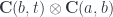


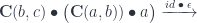
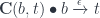


 , where
  .
.

 by injecting a pair of morphisms from the two hom-sets sharing the same
 ![\mathcal{C}(c \times b, t) \cong \mathcal{C}(c, [b, t])](https://s0.wp.com/latex.php?latex=%5Cmathcal%7BC%7D%28c+%5Ctimes+b%2C+t%29+%5Ccong+%5Cmathcal%7BC%7D%28c%2C+%5Bb%2C+t%5D%29&bg=ffffff&fg=29303b&s=0&c=20201002)
![\int^{c : \mathcal{C}} \mathcal{C}(s, c \times a) \times \mathcal{C}(c, [b, t]) \cong \mathcal{C}(s, [b, t] \times a) \cong \mathcal{C}(s \times b, t) \times \mathcal{C}(s, a)](https://s0.wp.com/latex.php?latex=%5Cint%5E%7Bc+%3A+%5Cmathcal%7BC%7D%7D+%5Cmathcal%7BC%7D%28s%2C+c+%5Ctimes+a%29+%5Ctimes+%5Cmathcal%7BC%7D%28c%2C+%5Bb%2C+t%5D%29+%5Ccong+%5Cmathcal%7BC%7D%28s%2C+%5Bb%2C+t%5D+%5Ctimes+a%29+%5Ccong+%5Cmathcal%7BC%7D%28s+%5Ctimes+b%2C+t%29+%5Ctimes+%5Cmathcal%7BC%7D%28s%2C+a%29&bg=ffffff&fg=29303b&s=0&c=20201002)


 , and further decompose
  , then you can decompose
  . Zooming-in is made possible by the associativity of the tensor product.
 to
to  is the optic
  . Zooming-in is the composition of morphisms.
 in
in 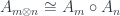

 is the unit object with respect to the tensor product
  is the identity endofunctor.)
 .
. in
in  in
in 
 . It’s a cross between a coproduct and a trace, as it’s constructed using injections of diagonal elements (with some identifications):
 :
: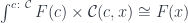
 , the base space
  , and a projection, or a display map,
  . The fibers of
  correspond to members of the type family. For instance, the total space, or the bundle, of counted vectors is the list type
  (a free monoid generated by
  ) with the projection
  that returns the length of a list.
 . Counted vectors, for instance, are represented as objects in
  given by pairs
  . Morphisms in the slice category correspond to fibre-wise mappings between bundles.
 has both the left adjoint, the dependent sum
  ; and the right adjoint, the dependent product
  . The base-change functor is defined as a pullback:
 and
and  . In a locally cartesian closed category, this product has the right adjoint, the internal hom in
 .
.


 are objects in the appropriate slice categories.
 on another object
  is given by the pullback:

![\cong \int^{\langle C, p \rangle : \mathcal{C}/B} (\mathcal{C}/B)( S, C \times_B A) \times (\mathcal{C}/B)(C , [A', S']_B)](https://s0.wp.com/latex.php?latex=%5Ccong+%5Cint%5E%7B%5Clangle+C%2C+p+%5Crangle+%3A+%5Cmathcal%7BC%7D%2FB%7D+%28%5Cmathcal%7BC%7D%2FB%29%28+S%2C+C+%5Ctimes_B+A%29+%5Ctimes+%28%5Cmathcal%7BC%7D%2FB%29%28C+%2C+%5BA%27%2C+S%27%5D_B%29+&bg=ffffff&fg=29303b&s=0&c=20201002)
![(\mathcal{C}/B)( S, [A', S']_B \times_B A)](https://s0.wp.com/latex.php?latex=%28%5Cmathcal%7BC%7D%2FB%29%28+S%2C+%5BA%27%2C+S%27%5D_B+%5Ctimes_B+A%29+&bg=ffffff&fg=29303b&s=0&c=20201002)
![[A', S']_B](https://s0.wp.com/latex.php?latex=%5BA%27%2C+S%27%5D_B&bg=ffffff&fg=29303b&s=0&c=20201002) in a locally cartesian closed category can be expressed using a dependent product:
in a locally cartesian closed category can be expressed using a dependent product:![\left [\left \langle A' \atop p \right \rangle, \left \langle S' \atop q \right \rangle \right ] \cong \Pi_p \left(p^* \left \langle S' \atop q \right \rangle \right)](https://s0.wp.com/latex.php?latex=%5Cleft+%5B%5Cleft+%5Clangle+A%27+%5Catop+p+%5Cright+%5Crangle%2C+%5Cleft+%5Clangle+S%27+%5Catop+q+%5Cright+%5Crangle+%5Cright+%5D+%5Ccong+%5CPi_p+%5Cleft%28p%5E%2A+%5Cleft+%5Clangle+S%27+%5Catop+q+%5Cright+%5Crangle+%5Cright%29&bg=ffffff&fg=29303b&s=0&c=20201002)
 is the fibration of
  is the right adjoint to the base change functor, and
  is the base-change functor along
 , this is equal to an infinite tuple of functions:
 indexed by
  .
.
 can be expressed as a fibration
  , with
  , the sum of the fibers. The set of powers of
  , with
  the type of list of
  the function that assigns the length to a list. The monoidal action can then be written using a product (pullback) in the slice category
  :
:
 , which can be used to express the polynomial action:


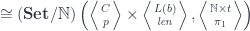
 is the projection from the cartesian product.
![(\mathbf{Set}/\mathbb{N})\left(\left \langle {C \atop p} \right \rangle, \left[ \left \langle {L(b) \atop \mathit{len}} \right \rangle, \left \langle {\mathbb{N} \times t \atop \pi_1} \right \rangle \right] \right)](https://s0.wp.com/latex.php?latex=%28%5Cmathbf%7BSet%7D%2F%5Cmathbb%7BN%7D%29%5Cleft%28%5Cleft+%5Clangle+%7BC+%5Catop+p%7D+%5Cright+%5Crangle%2C+%5Cleft%5B+%5Cleft+%5Clangle+%7BL%28b%29+%5Catop+%5Cmathit%7Blen%7D%7D+%5Cright+%5Crangle%2C+%5Cleft+%5Clangle+%7B%5Cmathbb%7BN%7D+%5Ctimes+t+%5Catop+%5Cpi_1%7D+%5Cright+%5Crangle+%5Cright%5D+%5Cright%29+&bg=ffffff&fg=29303b&s=0&c=20201002)
 and get:
![O(a, b; s, t) \cong \mathbf{Set} \left( s, U\left( \left[ \left \langle {L(b) \atop \mathit{len}} \right \rangle, \left \langle {\mathbb{N} \times t \atop \pi_1} \right \rangle \right] \times \left \langle {L(a) \atop \mathit{len}} \right \rangle \right) \right)](https://s0.wp.com/latex.php?latex=O%28a%2C+b%3B+s%2C+t%29+%5Ccong+%5Cmathbf%7BSet%7D+%5Cleft%28+s%2C+U%5Cleft%28+%5Cleft%5B+%5Cleft+%5Clangle+%7BL%28b%29+%5Catop+%5Cmathit%7Blen%7D%7D+%5Cright+%5Crangle%2C+%5Cleft+%5Clangle+%7B%5Cmathbb%7BN%7D+%5Ctimes+t+%5Catop+%5Cpi_1%7D+%5Cright+%5Crangle+%5Cright%5D+%5Ctimes+%5Cleft+%5Clangle+%7BL%28a%29+%5Catop+%5Cmathit%7Blen%7D%7D+%5Cright+%5Crangle+%5Cright%29+%5Cright%29+&bg=ffffff&fg=29303b&s=0&c=20201002)

 leaves: a traversal would return a list of leaves, and it would allow you to replace them with a new list. The problem is that the size of the list you pass to the setter cannot be arbitrary—it must match the number of leaves in the particular tree. This is why, in Haskell, the setter and the getter are usually combined in a single function:


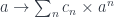
![\int^{c \colon [\mathbb{N}, \mathbf{Set}]} \mathbf{Set}\big(s, \sum_n c_n \times a^n\big) \times \mathbf{Set}\big( \sum_m c_m \times b^m, t\big)](https://s0.wp.com/latex.php?latex=%5Cint%5E%7Bc+%5Ccolon+%5B%5Cmathbb%7BN%7D%2C+%5Cmathbf%7BSet%7D%5D%7D+%5Cmathbf%7BSet%7D%5Cbig%28s%2C+%5Csum_n+c_n+%5Ctimes+a%5En%5Cbig%29+%5Ctimes+%5Cmathbf%7BSet%7D%5Cbig%28+%5Csum_m+c_m+%5Ctimes+b%5Em%2C+t%5Cbig%29+&bg=ffffff&fg=29303b&s=0&c=20201002)
![\int^{c \colon [\mathbb{N}, \mathbf{Set}]} \mathbf{Set}\big(s, \sum_n c_n \times a^n\big) \times \prod_m \mathbf{Set}\big( c_m \times b^m, t\big)](https://s0.wp.com/latex.php?latex=%5Cint%5E%7Bc+%5Ccolon+%5B%5Cmathbb%7BN%7D%2C+%5Cmathbf%7BSet%7D%5D%7D+%5Cmathbf%7BSet%7D%5Cbig%28s%2C+%5Csum_n+c_n+%5Ctimes+a%5En%5Cbig%29+%5Ctimes+%5Cprod_m+%5Cmathbf%7BSet%7D%5Cbig%28+c_m+%5Ctimes+b%5Em%2C+t%5Cbig%29+&bg=ffffff&fg=29303b&s=0&c=20201002)
![\int^{c \colon [\mathbb{N}, \mathbf{Set}]} \mathbf{Set}\big(s, \sum_n c_n \times a^n\big) \times \prod_m \mathbf{Set}\big( c_m, \mathbf{Set}( b^m, t)\big)](https://s0.wp.com/latex.php?latex=%5Cint%5E%7Bc+%5Ccolon+%5B%5Cmathbb%7BN%7D%2C+%5Cmathbf%7BSet%7D%5D%7D+%5Cmathbf%7BSet%7D%5Cbig%28s%2C+%5Csum_n+c_n+%5Ctimes+a%5En%5Cbig%29+%5Ctimes+%5Cprod_m+%5Cmathbf%7BSet%7D%5Cbig%28+c_m%2C+%5Cmathbf%7BSet%7D%28+b%5Em%2C+t%29%5Cbig%29+&bg=ffffff&fg=29303b&s=0&c=20201002)
![[\mathbb{N}, \mathbf{Set}]](https://s0.wp.com/latex.php?latex=%5B%5Cmathbb%7BN%7D%2C+%5Cmathbf%7BSet%7D%5D&bg=ffffff&fg=29303b&s=0&c=20201002)
![\int^{c \colon [\mathbb{N}, \mathbf{Set}]} \mathbf{Set}\big(s, \sum_n c_n \times a^n\big) \times [\mathbb{N}, \mathbf{Set}]\big( c_-, \mathbf{Set}( b^-, t)\big)](https://s0.wp.com/latex.php?latex=%5Cint%5E%7Bc+%5Ccolon+%5B%5Cmathbb%7BN%7D%2C+%5Cmathbf%7BSet%7D%5D%7D+%5Cmathbf%7BSet%7D%5Cbig%28s%2C+%5Csum_n+c_n+%5Ctimes+a%5En%5Cbig%29+%5Ctimes+%5B%5Cmathbb%7BN%7D%2C+%5Cmathbf%7BSet%7D%5D%5Cbig%28+c_-%2C+%5Cmathbf%7BSet%7D%28+b%5E-%2C+t%29%5Cbig%29+&bg=ffffff&fg=29303b&s=0&c=20201002)
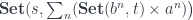

![F \colon \mathcal{M} \to [\mathcal{C}, \mathcal{C}]](https://s0.wp.com/latex.php?latex=F+%5Ccolon+%5Cmathcal%7BM%7D+%5Cto+%5B%5Cmathcal%7BC%7D%2C+%5Cmathcal%7BC%7D%5D+&bg=ffffff&fg=29303b&s=0&c=20201002)
![G \colon \mathcal{M} \to [\mathcal{D}, \mathcal{D}]](https://s0.wp.com/latex.php?latex=G+%5Ccolon+%5Cmathcal%7BM%7D+%5Cto+%5B%5Cmathcal%7BD%7D%2C+%5Cmathcal%7BD%7D%5D+&bg=ffffff&fg=29303b&s=0&c=20201002)


 into
into  . In physics, we would say that the paths are “invariant” under the transformation, but in category theory we are fine with a one-way mapping.
 , such a mapping exists, then these states are related. There exists a transformation and a pair of morphisms that are secretly used in the path integral to extend the original path.
 to
to  by first applying
  and then lifting the two morphisms. The converse is also true: if every path can be extended then such a pair of morphisms must exist.
 can be interpreted both as parameterizing a monoidal action and the residue left over after removing the focus.
 acting as the unit with respect to taking the end. It takes an
  and returns an
  that we’ve encountered before. They are parameterized by objects in

![\int_{x} \mathbf{Set}\big(\mathcal{C}(a, x), fx\big) = [\mathcal{C}, \mathbf{Set}]\big(\mathcal{C}(a, -), f\big)](https://s0.wp.com/latex.php?latex=%5Cint_%7Bx%7D+%5Cmathbf%7BSet%7D%5Cbig%28%5Cmathcal%7BC%7D%28a%2C+x%29%2C+fx%5Cbig%29+%3D+%5B%5Cmathcal%7BC%7D%2C+%5Cmathbf%7BSet%7D%5D%5Cbig%28%5Cmathcal%7BC%7D%28a%2C+-%29%2C+f%5Cbig%29&bg=ffffff&fg=29303b&s=0&c=20201002)
![[\mathcal{C}, \mathbf{Set}]\big(\mathcal{C}(s, -), \mathcal{C}(a, -) \big)](https://s0.wp.com/latex.php?latex=%5B%5Cmathcal%7BC%7D%2C+%5Cmathbf%7BSet%7D%5D%5Cbig%28%5Cmathcal%7BC%7D%28s%2C+-%29%2C+%5Cmathcal%7BC%7D%28a%2C+-%29+%5Cbig%29&bg=ffffff&fg=29303b&s=0&c=20201002)
 . The result is:
 , so a profunctor is defined a functor from
  to
to  to every pair

![[\mathcal{C}^{op} \times \mathcal{C}, \mathbf{Set}]](https://s0.wp.com/latex.php?latex=%5B%5Cmathcal%7BC%7D%5E%7Bop%7D+%5Ctimes+%5Cmathcal%7BC%7D%2C+%5Cmathbf%7BSet%7D%5D&bg=ffffff&fg=29303b&s=0&c=20201002) . We can immediately apply the double Yoneda identity to it to get:
. We can immediately apply the double Yoneda identity to it to get:


 . Let me explain.
![[\mathcal{C}, \mathbf{Set}]](https://s0.wp.com/latex.php?latex=%5B%5Cmathcal%7BC%7D%2C+%5Cmathbf%7BSet%7D%5D&bg=ffffff&fg=29303b&s=0&c=20201002) and endow it with some structure, resulting in another functor category
and endow it with some structure, resulting in another functor category  . It means that there is a (higher-order) forgetful functor
 ![U \colon \mathcal{T} \to [\mathcal{C}, \mathbf{Set}]](https://s0.wp.com/latex.php?latex=U+%5Ccolon+%5Cmathcal%7BT%7D+%5Cto+%5B%5Cmathcal%7BC%7D%2C+%5Cmathbf%7BSet%7D%5D&bg=ffffff&fg=29303b&s=0&c=20201002) that forgets this additional structure. We’ll also assume that there is the right adjoint functor
that forgets this additional structure. We’ll also assume that there is the right adjoint functor 
 is a functor in
![\int_{x \colon C} \mathbf{Set}\big(\mathcal{C}(a, x), (U f) x\big) = [\mathcal{C}, \mathbf{Set}]\big(\mathcal{C}(a, -), U f\big)](https://s0.wp.com/latex.php?latex=%5Cint_%7Bx+%5Ccolon+C%7D+%5Cmathbf%7BSet%7D%5Cbig%28%5Cmathcal%7BC%7D%28a%2C+x%29%2C+%28U+f%29+x%5Cbig%29+%3D+%5B%5Cmathcal%7BC%7D%2C+%5Cmathbf%7BSet%7D%5D%5Cbig%28%5Cmathcal%7BC%7D%28a%2C+-%29%2C+U+f%5Cbig%29&bg=ffffff&fg=29303b&s=0&c=20201002)
![[\mathcal{C}, \mathbf{Set}]\big(\mathcal{C}(a, -), U f\big) \cong \mathcal{T}\Big(F\big(\mathcal{C}(a, -)\big), f\Big)](https://s0.wp.com/latex.php?latex=%5B%5Cmathcal%7BC%7D%2C+%5Cmathbf%7BSet%7D%5D%5Cbig%28%5Cmathcal%7BC%7D%28a%2C+-%29%2C+U+f%5Cbig%29+%5Ccong+%5Cmathcal%7BT%7D%5CBig%28F%5Cbig%28%5Cmathcal%7BC%7D%28a%2C+-%29%5Cbig%29%2C+f%5CBig%29&bg=ffffff&fg=29303b&s=0&c=20201002)

![[\mathcal{C}, \mathbf{Set}] \Big( \mathcal{C}(s, -), (U \circ F)\big(\mathcal{C}(a, -)\big) \Big)](https://s0.wp.com/latex.php?latex=%5B%5Cmathcal%7BC%7D%2C+%5Cmathbf%7BSet%7D%5D+%5CBig%28+%5Cmathcal%7BC%7D%28s%2C+-%29%2C+%28U+%5Ccirc+F%29%5Cbig%28%5Cmathcal%7BC%7D%28a%2C+-%29%5Cbig%29+%5CBig%29+&bg=ffffff&fg=29303b&s=0&c=20201002)


 on the hom-functor
  . This is a monad in the functor category


 :
:
 .
.
 are given by natural transformations:
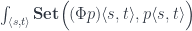


 with
with 
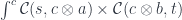
 (or
(or  stands for the set of arrows from
  in
in  stands for a set of functions from
  or, in Haskell
  can be expressed using the end notation:
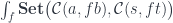
 , it becomes a functor, which is called a representable functor—the object
![[\mathcal{C},\mathbf{Set}]](https://s0.wp.com/latex.php?latex=%5B%5Cmathcal%7BC%7D%2C%5Cmathbf%7BSet%7D%5D&bg=ffffff&fg=29303b&s=0&c=20201002) . A hom-set in that category is a set of natural transformations between two functors which, as we’ve seen, can be expressed as an end:
. A hom-set in that category is a set of natural transformations between two functors which, as we’ve seen, can be expressed as an end: \cong \int_x \mathbf{Set}(f x, g x)](https://s0.wp.com/latex.php?latex=%5B%5Cmathcal%7BC%7D%2C%5Cmathbf%7BSet%7D%5D%28f%2C+g%29+%5Ccong+%5Cint_x+%5Cmathbf%7BSet%7D%28f+x%2C+g+x%29+&bg=ffffff&fg=29303b&s=0&c=20201002)
, [\mathcal{C},\mathbf{Set}](h, f)\big) \cong [\mathcal{C},\mathbf{Set}](h, g)](https://s0.wp.com/latex.php?latex=%5Cint_f+%5Cmathbf%7BSet%7D%5Cbig%28+%5B%5Cmathcal%7BC%7D%2C%5Cmathbf%7BSet%7D%5D%28g%2C+f%29%2C+%5B%5Cmathcal%7BC%7D%2C%5Cmathbf%7BSet%7D%5D%28h%2C+f%29%5Cbig%29+%5Ccong+%5B%5Cmathcal%7BC%7D%2C%5Cmathbf%7BSet%7D%5D%28h%2C+g%29+&bg=ffffff&fg=29303b&s=0&c=20201002)
 is all we need to finish the proof.

 corresponds to the function type
  . This is just saying that a function of two arguments is equivalent to a function returning a function.
 and
and  , where
  and
and  are some higher-order functors from
 , [\mathcal{C},\mathbf{Set}](L_t s, f)\big) \cong [\mathcal{C},\mathbf{Set}](L_t s, L_b a)](https://s0.wp.com/latex.php?latex=%5Cint_f+%5Cmathbf%7BSet%7D%5Cbig%28+%5B%5Cmathcal%7BC%7D%2C%5Cmathbf%7BSet%7D%5D%28L_b+a%2C+f%29%2C+%5B%5Cmathcal%7BC%7D%2C%5Cmathbf%7BSet%7D%5D%28L_t+s%2C+f%29%5Cbig%29+%5Ccong+%5B%5Cmathcal%7BC%7D%2C%5Cmathbf%7BSet%7D%5D%28L_t+s%2C+L_b+a%29+&bg=ffffff&fg=29303b&s=0&c=20201002)
 and
and  that go in the opposite direction from


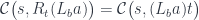
 \cong \mathcal{C}(a, R_b f) = \mathcal{C}(a, f b)](https://s0.wp.com/latex.php?latex=%5B%5Cmathcal%7BC%7D%2C%5Cmathbf%7BSet%7D%5D%28L_b+a%2C+f%29+%5Ccong+%5Cmathcal%7BC%7D%28a%2C+R_b+f%29+%3D+%5Cmathcal%7BC%7D%28a%2C+f+b%29&bg=ffffff&fg=29303b&s=0&c=20201002)


 translates to the function type


 . The breakthrough came with the realization that, if


 defined by the unique property of leaving things alone
 , which ignores one of its inputs


 happens to have a similar decomposition
 . The Twinklean industry was based on the principle of mass production; and mass production starts with duplication and reuse. Suppose you have a reusable part


 .
.


