There are many excellent AI papers and tutorials that explain the attention pattern in Large Language Models. But this essentially simple pattern is often obscured by implementation details and optimizations. In this post I will try to cut to the essentials.
In a nutshell, the attention machinery tries to get at a meaning of a word (more precisely, a token). This should be easy in principle: we could just look it up in the dictionary. For instance, the word “triskaidekaphobia” means “extreme superstition regarding the number thirteen.” Simple enough. But consider the question: What does “it” mean in the sentence “look it up in the dictionary”? You could look up the word “it” in the dictionary, but that wouldn’t help much. More ofthen than not, we guess the meaning of words from their context, sometimes based on a whole conversation.
The attention mechanism is a way to train a language model to be able to derive a meaning of a word from its context.
The first step is the rough encoding of words (tokens) as multi-dimensional vectors. We’re talking about 12,288 dimensions for GPT-3. That’s an enormous semantic space. It means that you can adjust the meaning of a word by nudging it in thousands of different directions by varying amounts (usually 32-bit floating point numbers). This “nudging” is like adding little footnotes to a word, explaining what was its precise meaning in a particular situation.
(Note: In practice, working with such huge vectors would be prohibitively expensive, so they are split between multiple heads of attention and processed in parallel. For instance, GPT-3 has 96 heads of attention, and each head works within a 128-dimensional vector space.)
We are embedding the input word as a 12,288-dimensional vector 


(Note: In most descriptions, you’ll see a whole batch of words begin embedded all at once, and the context often being identical with that same batch–but this is just an optimization.)
The goal is to refine the embedding 
This is usually described as the vector
First, we apply a gigantic trainable 12,288 by 12,288 matrix 

You may think of 
We then apply another trainable matrix 

You may think of 


The next step is crucial: We calculate how relevant each element of the context is to our word. In other words, we are focusing our attention on particular elements of the context. We do it by taking 
A scalar product can vary widely. A large positive number means that the
What we really need is to normalize these numbers to a range between zero (not relevant) and one (extremely relevant) and make sure that they all add up to one. This is normally done using the softmax procedure: we first raise 

We then divide it by the total sum, to normalize it:

These are our attention weights. (Note: For efficiency, before performing the softmax, we divide all numbers by the square root of the dimension of the vector space 

Attention weights tell us how much each element of the context can contribute to the meaning of 


We now accumulate all these contribution, weighing them by their attention weights 

The result 

And that’s essentially the basic block of the attention system. The rest is just optimization and composition.
One major optimization is gained by processing a whole window of tokens at once (2048 tokens for GPT-3). In particular, in the self-attention pattern we use the same batch of tokens for both the input and the context. In general, though, the context can be distinct from the input. It could, for instance, be a sentence in a different language.
Another optimization is the partitioning of all three vectors,
In GPT-3, each multi-headed attention block is followed by a multi-layer perceptron, MLP, and this transformation is repeated 96 times. Most steps in an LLM are just linear algebra; except for softmax and the activation function in the MLP, which are non-linear.
All this work is done just to produce the next word in a sentence.
 :
:
 is an object of
 .
. is a category in which we define an action of a monoidal category

 and
and  . The first constructs parametric morphisms from
  to
to  as
as 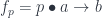 , and the second as
  .
.
 are objects of some monoidal category
  , and the parameters
  come from another monoidal category
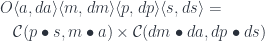
 in
in  to the pair of objects
  also in
  in
in  and a pair
  .
. for the category
  , and bold letters for pairs of objects and (twisted) pairs of morphisms. For instance,
  is a member of the hom-set
  represented by a pair
  .
. to denote the monoidal action of
  on
on 


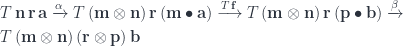
 bicategory. The composition is a mapping:
 and the second by
  :
:


 ,
,  , and
, and  .
.
 and
and  . Associativity and identity laws are satisfied modulo the associators and the unitors.
 bicategory is also monoidal, with the obvious point-wise parallel composition of pre-optics.


 to
to  must give the same result.
 .
. , we get regular Tambara modules.
 , we can define a mapping
  from the triple:
 by
by  and rearranging the actions using their commutativity.
 , we map:

 can be expressed using triple Tambara modules. An optic:
 and get an arbitrary pre-optic.