I was originally attracted to category theory when trying to understand Haskell optics. I was puzzled by the van Laarhoven’s functor representations and Kmett’s use of Tambara modules. By playing Tetris with the Yoneda lemma I was able to make some progress, attacking more and more esoteric topics. With a group of researcher and students at the Oxford Adjoint School in Applied Category Theory we cracked the problem of traversal optics and published a paper summarizing the advances in profunctor optics.
Optics sit at an intersection of monoidal actions and Tambara modules. There is a duality between optics and Tambara representations. It is related to what mathematicians call Tannakian reconstruction, when an algebraic object is recovered from the totality of its representations.
No wonder then that a recent article by Mateusz Stroiński, Module categories, internal bimodules and Tambara modules, piqued my interest. It turns out that Tambara modules can be thought of as horizontal arrows in a double category, which is also a proarrow equipment. I will try to sketch the contents of this paper and illustrate it using Haskell code.
The slogan is that Tambara modules are to monoidal functors as profunctors are to functors.
The main advantage of the double-categorical setting for Tambara modules is that it works out of the box for enriched categories.
Monoidal functors redux
For simplicity, I’ll be using a simplified version of a strict monoidal functor, which omits the object constraint from the definition of a monoidal category:
class (Actegory ten act1, Actegory ten act2, Functor f) => MonFunctor ten act1 act2 f where alpha :: m `act2` f a -> f (m `act1` a) alpha' :: f (m `act1` a) -> m `act2` f a
Here, alpha' is the inverse of alpha.
Monoidal functors compose:
newtype MonFunCompose f g a = MonFunCompose { getMonFunCompose :: f (g a) }
and the composition is again a monoidal functor:
instance ( Actegory ten act1 , Actegory ten act2 , Actegory ten act3 , MonFunctor ten act2 act3 f , MonFunctor ten act1 act2 g) => MonFunctor ten act1 act3 (MonFunCompose f g) where alpha mfga = let m3fga' = second getMonFunCompose mfga fmga = alpha @ten @act2 @act3 m3fga' fgma = fmap (alpha @ten @act1 @act2) fmga in MonFunCompose fgma alpha' (MonFunCompose fgma) = let fmga = fmap (alpha' @ten @act1 @act2) fgma mfga = alpha' @ten @act2 @act3 fmga in second MonFunCompose mfga
Notice the use of type application to help the Haskell type checker.
Tambara modules
A Tambara module is a profunctor that is compatible with the action of a monoidal category. If you interpret a profunctor as a proof-relevant relation, a Tambara module has the property that, whenever two objects are related, they remain related when you “multiply” them by the same object 


that is natural in 


(modulo some associators and unitors).
We can illustrate this in Haskell as a typeclass:
class (Actegory ten act, Profunctor j) => Tambara ten act j where leftAct :: j a b -> j (m `act` a) (m `act` b)
I chose to concentrate on the left action of the actegory, but it’s easy to define the right action, or both. For simplicity, I’m using the same action for both arguments. In full generality, we would have two separate actegories.
The simplest example of a Tambara module is the hom-functor:
instance (Actegory ten act) => Tambara ten act (->) where leftAct :: Actegory ten act => (a -> b) -> m `act` a -> m `act` b leftAct = second
Here I used the bifunctoriality of the action.
Tambara modules form a category, in which action-preserving natural transformations act as morphisms.
The usual profunctor composition using coends also works on Tambara modules.
data TamCompose p q d c where TamCompose :: p x c -> q d x -> TamCompose p q d c
The result of composition is again a Tambara module:
instance (Tambara ten act p, Tambara ten act q) => Tambara ten act (TamCompose p q) where leftAct :: (Tambara ten act p, Tambara ten act q) => TamCompose p q a b -> TamCompose p q (m `act` a) (m `act` b) leftAct (TamCompose pxc qdx) = TamCompose (leftAct pxc) (leftAct qdx)
Taken together, we have a bicategory 
Moreover, endo-Tambara modules, that is Tambara modules that operate within a single category, form a monoidal bicategory, with profunctor composition acting as a tensor product and a hom-functor acting as a unit.
Tambara Equipment
We have previously studied a double category 
It turns out that there is an analogous construction with actegories as 0-cells, Tambara modules as horizontal 1-cells, and monoidal functors as vertical 1-cells. To form 2-cells, we first have to be able to lift (or restrict) a Tambara module along a pair of monoidal functors. We define a lifting of 

or, using placeholders, 
newtype Lift f g j a c = Lift (j (f a) (g c))
The lifting of a Tambara module is again a Tambara module with the structure map defined as a composition:

The second arrow lifts the (invertible) monoidal functor structure map to

Here’s the same thing in Haskell:
instance ( Actegory ten act1 , Actegory ten act2 , MonFunctor ten act1 act2 f , MonFunctor ten act1 act2 g , Tambara ten act2 j) => Tambara ten act1 (Lift f g j) where leftAct (Lift j) = Lift $ dimap alpha' alpha $ leftAct @ten @act2 j
I used type applications to select the correct left action corresponding to act2.
A 2-cell is then a natural transformation from 

Or, in Haskell:
type Cell f g h j = forall a c . h a c -> j (f a) (g c)
The companion and the conjoint are representable profunctors, that are automatically Tambara modules as long as f is a monoidal functor (the Identity functor is trivially monoidal):
type Companion f d c = Lift f Identity (->)type Conjoint f d c = Lift Identity f (->)
The unit and counit cells for the companion and the conjoint are reasonably easy to define (see the linked code).
Free Tambara and Optics
There is an obvious forgetful functor from 


In Haskell, we model it as an existential data type:
data FreeTamb ten act j s t = forall m x y. (MonoidalCategory ten, Actegory ten act) => FreeTamb (s -> m `act` x) (j x y) (m `act` y -> t)
The result is indeed a Tambara module:
instance (Actegory ten act, MonoidalCategory ten, Profunctor j) => Tambara ten act (FreeTamb ten act j) where -- na -> (nm)c, jcd, (nm)d -> nb leftAct (FreeTamb a_mc jcd md_b) = FreeTamb f jcd g where --f :: n `act` a -> (n `ten` m) `act` c f na = assoc' $ second a_mc na --g :: (n `ten` m) `act` d -> n `act` b g nm_d= second md_b $ assoc nm_d
It so happens that optics can be defined as a free Tambara module acting on a representable profunctor 

In Haskell
data Rep a b x y = Rep (x -> a) (b -> y)
giving us:
type Optic ten s t a b = FreeTamb ten (Rep a b) s t
which, by Yoneda reduction, is isomorphic to:
data Optic ten act s t a b = forall m. Optic (s -> m `act` a) (m `act` b -> t)
Internalizing monoidal actions
A monoidal action, seen as a functor ![\mathbf M \to [C, C]](https://s0.wp.com/latex.php?latex=%5Cmathbf+M+%5Cto+%5BC%2C+C%5D&bg=ffffff&fg=29303b&s=0&c=20201002)


If you think of the action as “multiplication,” the adjunction is reminiscent of currying, and the right adjoint plays to role on the “internal hom.”
In Haskell, we define a typeclass:
class (Actegory ten act, MonoidalCategory ten, Profunctor hom) => IntHom ten act hom | hom -> act where icurry :: (m `act` a -> b) -> (m -> hom a b) iuncurry :: (m -> hom a b) -> (m `act` a -> b)
We can use this adjunction to simplify multiplicative optics:

Using the Yoneda reduction (a.k.a, “integrating” over

With additive optics, we use the right adjoint to coproduct to produce hom-sets in a product category.
Both tricks are used in simplifying traversals, which are optics generated by polynomial functors:
![\int^{c \colon [\mathbb N , Set]} C(s, \sum_n c_n \times a^n) \times C (\sum_m c_m \times b^m, t)](https://s0.wp.com/latex.php?latex=%5Cint%5E%7Bc+%5Ccolon+%5B%5Cmathbb+N+%2C+Set%5D%7D+C%28s%2C+%5Csum_n+c_n+%5Ctimes+a%5En%29+%5Ctimes+C+%28%5Csum_m+c_m+%5Ctimes+b%5Em%2C+t%29&bg=ffffff&fg=29303b&s=0&c=20201002)
Here, 


We first use the coproduct adjunction:

and follow it by the currying adjunction. We get the formula for a traversal:

The result can be illustrated in Haskell by replacing powers with lists:
type Traversal s t a b = s -> ([b] -> t, [a])
Internal monoid
The endo-hom 

The right hand side can be implemented as a double application of the counit of the adjunction:

In Haskell, we first define a monoid internal to a monoidal category:
class (MonoidalCategory ten) => IMonoid ten m where imempty :: Unit ten -> m imappend :: m `ten` m -> m
and show that hom a a is an instance of it:
instance (Actegory ten act, MonoidalCategory ten, IntHom ten act hom) => IMonoid ten (hom a a) where imempty = icurry unit -- imappend :: (hom a a) `ten` (hom a a) -> hom a a imappend = icurry (eval . second eval . assoc)
where counit of the adjunction is the eval function:
eval :: (Actegory ten act, MonoidalCategory ten, IntHom ten act hom) => hom a b `act` a -> beval = iuncurry id
Haskell code for this blog post is available here.
 , where
  . Similarly, a graph of a relation is a set of pairs where
  . If the set is empty, it means that the objects are unrelated.
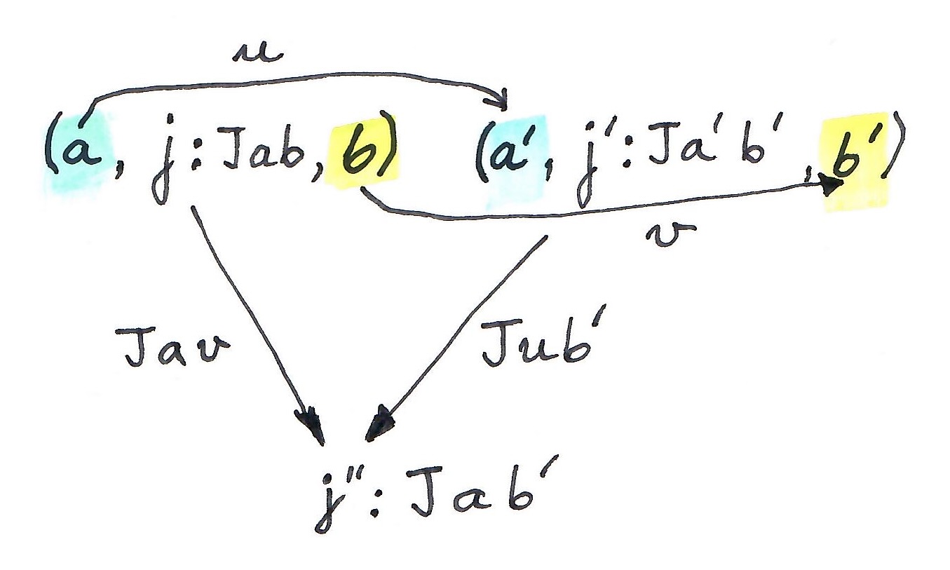
 , an object in the category of elements is a triple
  . We interpret
  as a witness that
  is a pair of morphisms
  such that:
 is the whiskering, or the lifting of a pair of morphisms, one of which is an identity, by the profunctor
  . We want the result, in both cases, to give us the same element of
  — the witness that
  .
.
 is a 0-cell
  equipped with two projections. Think of these projections as extracting the two objects from the triple that we used in the definition of a graph of a profunctor. Their relation to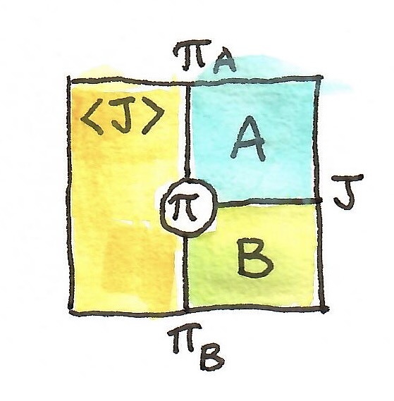

 is a natural transformation whose components are:
 and the result is an element of the set
  .
.  or
or  , both leading to the same result.
 . We postulate that for any 0-cell
  and
and  there is a unique factorization through the universal 2-cell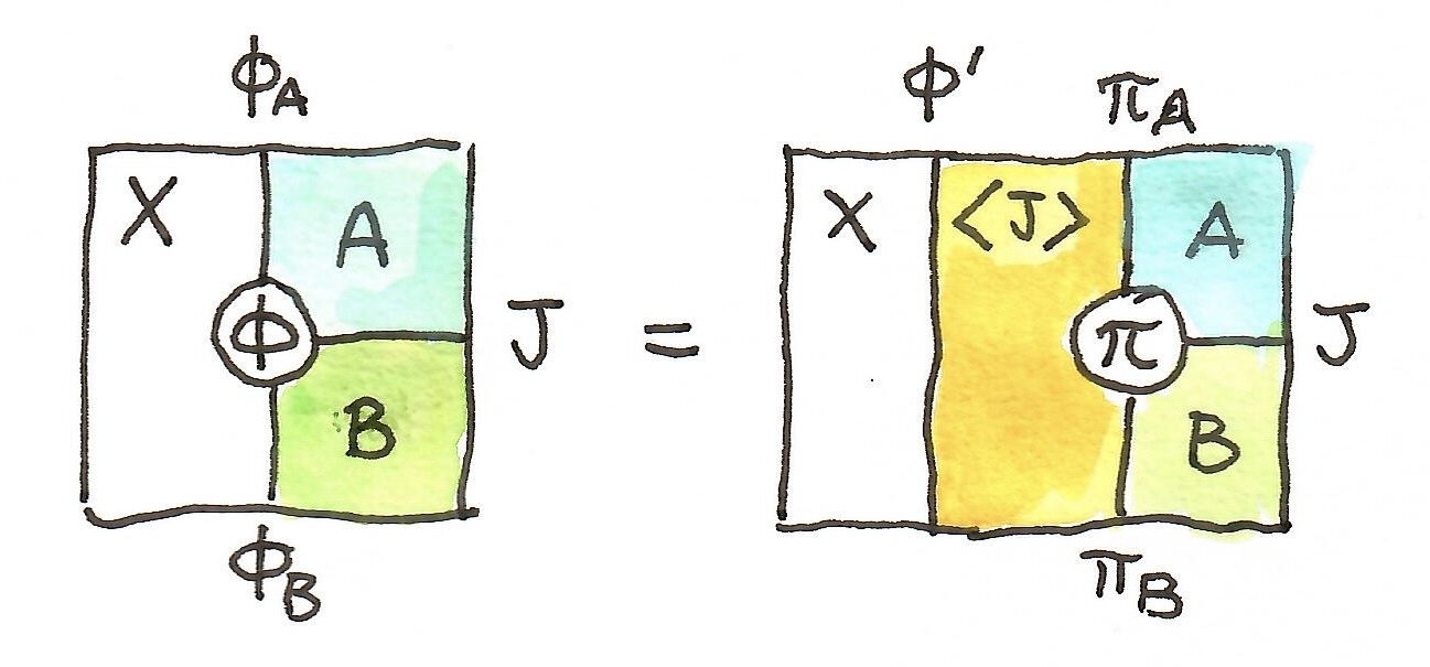


 , on objects, as:
 , as
, as  .
. . All we have to provide is two vertical arrows and a 2-cell. But to complete the picture, we should be able to construct a 2-cell from another horizontal 1-cell,
  together with a projection
  , such that: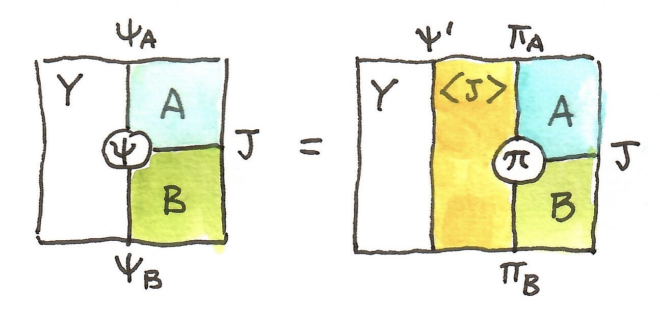
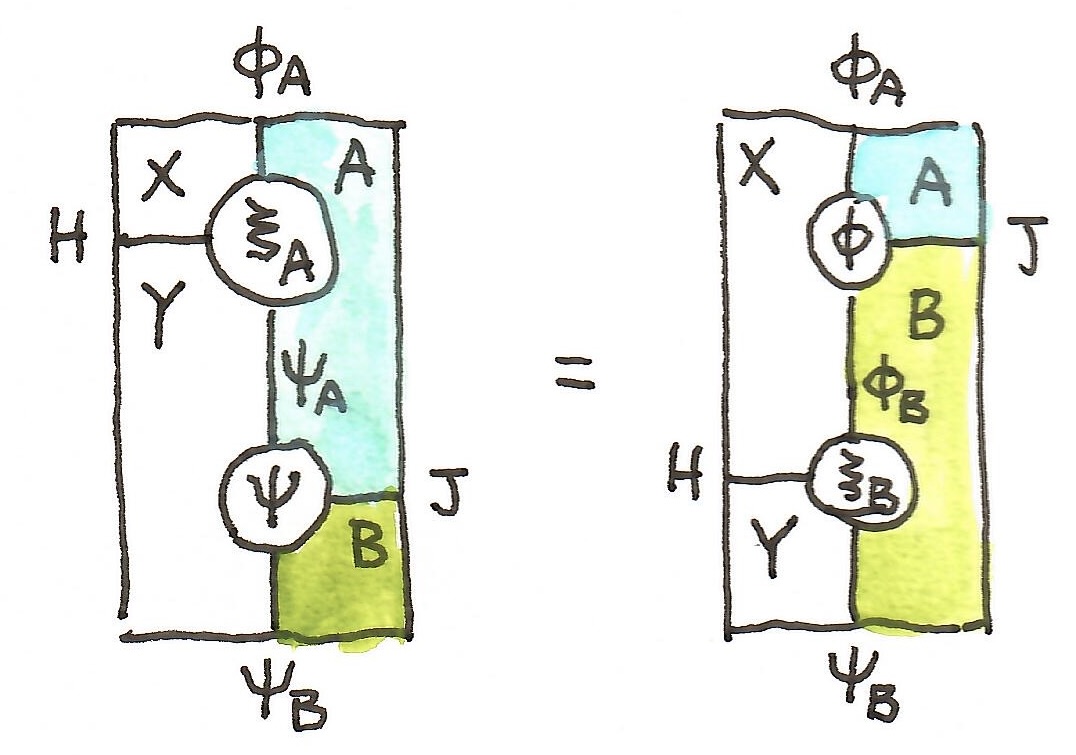


 :
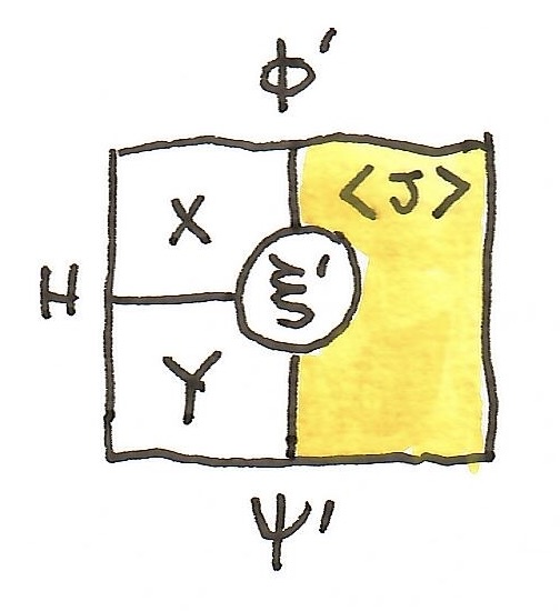
:
 and
and  factor through it. Here’s the first factorization: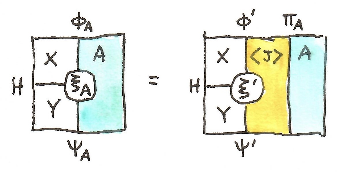

 , we get as the target a pair of morphisms:
 , we can construct such a pair as:
 this produces
  thus satisfying the 2-dimensional universal condition. The constraints on
  with
with  .
. that is somehow related to a vertical arrow
  . There are two 2-cells that illustrate this relation, but it’s not clear what their meaning is or how to use them.
 . Diagrammatically, we have:
 , is illustrated by the following diagrams:

 and
and  and turns them into
  and
and  . Then we shove the two counits below it (vertically postcompose), to bend the arrows
  and
and  .
.  and
and  , a cartesian square defines a horizontal arrow
  also called a restriction of
 . To this end we replace
  , together with two new vertical arrows
  and
and  that, just like
 to
to  over a pair of 1-cells
  , given the corresponding cartesian square
  .
.