November 16, 2024

Sieves and Sheaves

Posted by Bartosz Milewski under Category Theory, Topology | Tags: Category Theory, math, mathematics, Topology |
Leave a Comment

Previously: Covering Sieves.

We’ve seen an intuitive description of presheaves as virtual objects. We can use the same trick to visualize natural transformations.

A natural transformation can be drawn as a virtual arrow $\alpha$ between two virtual objects corresponding to two presheaves $S$ and $P$ . Indeed, for every $s_a \in S a$ , seen as an arrow $a \to S$ , we get an arrow $a \to P$ simply by composition $\alpha \circ s_a$ . Notice that we are thus defining the composition with $\alpha$ , because we are outside of the original category. A component $\alpha_a$ of a natural transformation is a mapping between two arrows.

Untitled Artwork

This composition must be associative and, indeed, associativity is guaranteed by the naturality condition. For any arrow $f \colon a \to b$ , consider a zigzag path from $a$ to $P$ given by $\alpha \circ s_b \circ f$ . The two ways of associating this composition give us $\alpha_a \circ S f = P f \circ \alpha_b$ .

Untitled Artwork

Let’s now recap our previous definitions: A cover of $u$ is a bunch of arrows converging on $u$ satisfying certain conditions. These conditions are defined in terms of a coverage. For every object $u$ we define a whole family of covers, and then combine them into one big collection that we call the coverage.

A sheaf is a presheaf that is compatible with a coverage. It means that for every cover $\{u_i\}$ , if we pick a compatible family of $x_i \in P u_i$ that agrees on all overlaps, then this uniquely determines the element (virtual arrow) $x \in P u$ .

Untitled Artwork

A covering sieve of $u$ is a presheaf that extends a cover $\{u_i\}$ . It assigns a singleton set to each $u_i$ and all its open subsets (that is objects that have arrows pointing to $u_i$ ); and an empty set otherwise. In particular, the sieve includes all the overlaps, like $u_i \cap u_j$ , even if they are not present in the original cover.

The key observation here is that a sieve can serve as a blueprint for, or a skeleton of, a compatible family $\{ x_i \}$ . Indeed, $S_u$ maps all objects either to singletons or to empty sets. In terms of virtual arrows, there is at most one arrow going to $S_u$ from any object. This is why a natural transformation from $S_u$ to any presheaf $P$ produces a family of arrows $x_i \in P u_i$ . It picks a single arrow from each of the hom-sets $u_i \to P$ .

Untitled Artwork

The sieve includes all intersections, and all diagrams involving those intersections necessarily commute. They commute because the category we’re working with is thin, and so is the category extended by adding the virtual object $S_u$ . Thus a family generated by a natural transformation $\alpha \in Nat (S_u, P)$ is automatically a compatible family. Therefore, if $P$ is a sheaf, it determines a unique element $x \in P u$ .

This lets us define a sheaf in terms of sieves, rather than coverages.

A presheaf $P$ is a sheaf if and only if, for every covering sieve $S_u$ of every $u$ , there is a one-to-one correspondence between the set of natural transformations $Nat (S_u, P)$ and the set $P u$ .

In terms of virtual arrows, this means that there is a one-to-one correspondence between arrows $\alpha \colon S_u \to P$ and $x \colon u \to P$ .

Untitled Artwork
Next: Subobject Classifier

October 31, 2024

Covering Sieves

Posted by Bartosz Milewski under Category Theory, Topology | Tags: Category Theory, math, mathematics, Topology |
[2] Comments

Previously: Sheaves as Virtual Objects.

In order to define a sheaf, we have to start with coverage. A coverage defines, for every object $u$ , a family of covers that satisfy the sub-coverage conditions. Granted, we can express coverage using objects and arrows, but it would be much nicer if we could use the language of functors and natural transformations.

Let’s start with the idea that, categorically, a cover of $u$ is a bunch of arrows converging on $u$ . Each arrow $p_i \colon u_i \to u$ is a member of the hom-set $\mathcal C (u_i, u)$ . Now consider the fact that $\mathcal C (-, u)$ is a presheaf, $\mathcal C^{op} \to \mathbf{Set}$ , and ask the question: Is a cover a “subfunctor” of $\mathcal C (-, u)$ ?

A subfunctor of a presheaf $P$ is defined as a functor $S$ such that, for each object $v$ , $S v$ is a subset of $P v$ and, for each arrow $f \colon v \to w$ , the function $S f \colon S w \to S v$ is a restriction of $P f$ .

Untitled Artwork

In general, a cover does not correspond to a subfunctor of the hom-functor. Let’s see why, and how we can fix it.

Let’s try to define $S$ , such that $S u_i$ is non-empty for any object $u_i$ that’s in the cover of $u$ , and empty otherwise. As a presheaf, we could represent it as a virtual object with arrows coming from all $\{ u_i \}$ ‘s.

Untitled Artwork

Now consider an object $v$ that is not in the cover, but it has an arrow $f \colon v \to u_k$ connecting it to some element $u_k$ of the cover. Functoriality requires the (virtual) composition $s_k \circ f$ to exist. Untitled Artwork

Thus $v$ must be included in the cover–if we want $S$ to be a functor.

In particular, if we are looking at a category of open sets with inclusions, this condition means that all (open) sub-sets of the covering sets must also be included in the cover. Such a “downward closed” family of sets is called a sieve.

Imagine sets in the cover as holes in a sieve. Smaller sets that can “pass through” these holes must also be parts of the sieve.

If you start with a cover, you can always extend it to a covering sieve by adding more arrows. It’s as if you started with a few black holes, and everything that could fall into them, would fall.

We have previously defined sheaves in terms of coverings. In the next installment we’ll see that they can equally well be defined using covering sieves.

Next Sieves and Sheaves.

October 24, 2024

Sheaves as Virtual Objects

Posted by Bartosz Milewski under Category Theory, Topology | Tags: Category Theory, math, mathematics, Topology |
1 Comment

Previously: Coverages and Sites

The definition of a sheaf is rather complex and involves several layers of abstraction. To help us navigate this maze we can use some useful intuitions. One such intuition is to view objects in our category as some kind of sets (in particular, open sets, when we talk about topology), and arrows as set inclusions. An arrow from $v$ to $u$ means that $v$ is a subset of $u$ .

A cover of $u$ is a family of arrows $\{ p_i \colon u_i \to u \}$ . A coverage assigns a collection of covers to every object, satisfying the sub-coverage conditions described in the previous post. A category with coverage is called a site.

The next layer of abstraction deals with presheaves, which are set-valued contravariant functors. Interestingly, there is a way to interpret a presheaf as an extension of the original category. I learned this trick from Paolo Perrone.

We may represent a presheaf $P$ using virtual hom-sets. First we add one virtual object, let’s call it $\bullet$ , to our category. The set $P u$ is then interpreted as the set of arrows from $u$ to $\bullet$ .

Untitled Artwork

Moreover, we can represent the action of $P$ on arrows as simple composition. Take an arrow $f \colon v \to u$ . The presheaf lifts it to a function between sets: $P f \colon P u \to P v$ (contravariance means that the arrow is reversed). For any $h \in P u$ we can define the composition $h \circ f$ to be $(P f) h$ .

Untitled Artwork

Incidentally, if the functor $P$ is representable, it means that we can replace the virtual object $\bullet$ with an actual object in our category.

Notice that, even though the category of open sets with inclusions is a poset (hom-sets are either singletons or empty, and all diagrams automatically commute), the added virtual hom-sets usually contain lots of arrows. In topology these hom-sets are supposed to represent sets of continuous functions over open sets.

We can interpret the virtual object $\bullet$ as representing an imaginary open set that “includes” all the objects $u$ for which $P u$ is non-empty, but we have to imagine that it’s possible to include an object in more than one way, to account for multiple arrows. In fact, in what follows we won’t be assuming that the underlying category is a poset, so virtual hom-sets are nothing special.

To express the idea of intersections of open sets, we use commuting diagrams. For every pair of objects $u_i$ and $u_j$ that are in the cover of $u$ , an object $v$ is in their intersection if the following diagram commutes:

Untitled Artwork

Note that in a poset all diagrams commute, but here we’re generalizing this condition to an arbitrary category. We could say that $v$ is in the intersection of $u_i$ and $u_j$ seen as covers of $u$ .

Equipped with this new insight, we can now express the sheaf condition. We assume that there is a coverage defined in our category. We are adding one more virtual object $\bullet$ for the presheaf $P$ , with bunches of virtual arrows pointing to it.

For every cover $\{ p_i \colon u_i \to u \}$ we try to select a family of virtual arrows, $s_i \colon u_i \to \bullet$ . It’s as if the objects $u_i$ , besides covering $u$ , also covered the virtual object $\bullet$ .

We call the family $\{s_i \}$ a matching family, if this new covering respects the existing intersections. If $v$ is in the intersection of $u_i$ and $u_j$ (as covers of $u$ , see the previous diagram), then we want the following diagram to also commute:
Untitled Artwork
In other words, the $\{u_i\}$ ‘s intersect as covers of $\bullet$ .

A presheaf $P$ is a sheaf if, for every covering family $p_i$ and every matching family $s_i$ there exists a unique $s \colon u \to \bullet$ that factorizes those $s_i$ ‘s:
Untitled Artwork
Translating it back to the language of topology: There is a unique global function $s$ defined over $u$ whose restrictions are $s_i$ ‘s.

The advantage of this approach is that it’s easy to imagine the sheafification of an arbitrary presheaf by freely adding virtual arrows (the $s$ ‘s and their compositions with $p_i$ ‘s in the above diagram) to all intersection diagrams.

Next: Covering Sieves

February 7, 2024

Linear Lenses in Haskell

Posted by Bartosz Milewski under Programming | Tags: Category Theory, education, Functional Programming, hinduism, mathematics, Optics, Profunctors, Tambara Modules |
[3] Comments

I always believed that the main problems in designing a programming language were resource management and concurrency–and the two are related. If you can track ownership of resources, you can be sure that no synchronization is needed when there’s a single owner.

I’ve been evangelizing resource management for a long time, first in C++, and then in D (see Appendix 3). I was happy to see it implemented in Rust as ownership types, and I’m happy to see it coming to Haskell as linear types.

Haskell has essentially solved the concurrency and parallelism problems by channeling mutation to dedicated monads, but resource management has always been part of the awkward squad. The main advantage of linear types in Haskell, other than dealing with external resources, is to allow safe mutation and non-GC memory management. This could potentially lead to substantial performance gains.

This post is based on very informative discussions I had with Arnaud Spiwack, who explained to me the work he’d done on linear types and linear lenses, some of it never before documented.

The PDF version of this post together with complete Haskell code is available on GitHub.

Linear types

What is a linear function? The short answer is that a linear function $a \multimap b$ “consumes” its argument exactly once. This is not the whole truth, though, because we also have linear identity $id_a \colon a \multimap a$ , which ostensibly does not consume $a$ . The long answer is that a linear function consumes its argument exactly once if it itself is consumed exactly once, and its result is consumed exactly once.

What remains to define is what it means to be consumed. A function is consumed when it’s applied to its argument. A base value like Int or Char is consumed when it’s evaluated, and an algebraic data type is consumed when it’s pattern-matched and all its matched components are consumed.

For instance, to consume a linear pair (a, b), you pattern-match it and then consume both a and b. To consume Either a b, you pattern-match it and consume the matched component, either a or b, depending on which branch was taken.

As you can see, except for the base values, a linear argument is like a hot potato: you “consume” it by passing it to somebody else.

So where does the buck stop? This is where the magic happens: Every resource comes with a special primitive that gets rid of it. A file handle gets closed, memory gets deallocated, an array gets frozen, and Frodo throws the ring into the fires of Mount Doom.

To notify the type system that the resource has been destroyed, a linear function will return a value inside the special unrestricted type Ur. When this type is pattern-matched, the original resource is finally destroyed.

For instance, for linear arrays, one such primitive is toList:

$\mathit{toList} \colon \text{Array} \; a \multimap \text{Ur} \, [a]$

In Haskell, we annotate the linear arrows with multiplicity 1:

toList :: Array a %1-> Ur  [a]

Similarly, magic is used to create the resource in the first place. For arrays, this happens inside the primitive fromList.

$\mathit{fromList} \colon [a] \to (\text{Array} \; a \multimap \text{Ur} \; b) \multimap \text{Ur} \; b$

or using Haskell syntax:

fromList :: [a] -> (Array a %1-> Ur b) %1-> Ur b

The kind of resource management I advertised in C++ was scope based. A resource was encapsulated in a smart pointer that was automatically destroyed at scope exit.

With linear types, the role of the scope is played by a user-provided linear function; here, the continuation:

(Array a %1 -> Ur b)

The primitive fromList promises to consume this user-provided function exactly once and to return its unrestricted result. The client is obliged to consume the array exactly once (e.g., by calling toList). This obligation is encoded in the type of the continuation accepted by fromList.

Linear lens: The existential form

A lens abstracts the idea of focusing on a part of a larger data structure. It is used to access or modify its focus. An existential form of a lens consists of two functions: one splitting the source into the focus and the residue; and the other replacing the focus with a new value, and creating a new whole. We don’t care about the actual type of the residue so we keep it as an existential.

The way to think about a linear lens is to consider its source as a resource. The act of splitting it into a focus and a residue is destructive: it consumes its source to produce two new resources. It splits one hot potato s into two hot potatoes: the residue c and the focus a.

Conversely, the part that rebuilds the target t must consume both the residue c and the new focus b.

We end up with the following Haskell implementation:

data LinLensEx a b s t where
  LinLensEx :: (s %1-> (c, a)) -> 
               ((c, b) %1-> t) -> LinLensEx a b s t

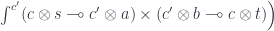
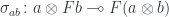
A Haskell existential type corresponds to a categorical coend, so the above definition is equivalent to:

$L a b s t = \int^c (s \multimap c \otimes a)\times (c \otimes b \multimap t)$

I use the lollipop notation for the hom-set in a monoidal category with a tensor product $\otimes$ .

The important property of a monoidal category is that its tensor product doesn’t come with a pair of projections; and the unit object is not terminal. In particular, a morphism $s \multimap c \otimes a$ cannot be decomposed into a product of two morphisms $(s \multimap c) \times (s \multimap a)$ .

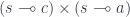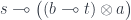
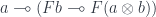
However, in a closed monoidal category we can curry a mapping out of a tensor product:

$c \otimes b \multimap t \cong c \multimap (b \multimap t)$

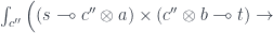
We can therefore rewrite the existential lens as:

$L a b s t \cong \int^c (s \multimap c \otimes a)\times (c \multimap (b \multimap t))$

and then apply the co-Yoneda lemma to get:

$s \multimap \big((b \multimap t) \otimes a\big)$

Unlike the case of a standard lens, this form cannot be separated into a get/set pair.

The intuition is that a linear lens lets you consume the object $s$ , but it leaves you with the obligation to consume both the setter $b \multimap t$ and the focus $a$ . You can’t just extract $a$ alone, because that would leave a gaping hole in your object. You have to plug it in with a new object $b$ , and that’s what the setter lets you do.

Here’s the Haskell translation of this formula (conventionally, with the pairs of arguments reversed):

type LinLens s t a b = s %1-> (b %1-> t, a)

The Yoneda shenanigans translate into a pair of Haskell functions. Notice that, just like in the co-Yoneda trick, the existential $c$ is replaced by the linear function $b \multimap t$ .

fromLinLens :: forall s t a b.
  LinLens s t a b -> LinLensEx a b s t
fromLinLens h = LinLensEx f g
  where
    f :: s %1-> (b %1-> t, a)
    f = h
    g :: (b %1-> t, b) %1-> t
    g (set, b) = set b

The inverse mapping is:

toLinLens :: LinLensEx a b s t -> LinLens s t a b
toLinLens (LinLensEx f g) s = 
  case f s of
    (c, a) -> (\b -> g (c, b), a)

Profunctor representation

Every optic comes with a profunctor representation and the linear lens is no exception. Categorically speaking, a profunctor is a functor from the product category $\mathcal C^{op} \times \mathcal C$ to $\mathbf{Set}$ . It maps pairs of object to sets, and pairs of morphisms to functions. Since we are in a monoidal category, the morphisms are linear functions, but the mappings between sets are regular functions (see Appendix 1). Thus the action of the profunctor $p$ on morphisms is a function:

$(a' \multimap a) \to (b \multimap b') \to p a b \to p a' b'$

In Haskell:

class Profunctor p where
  dimap :: (a' %1-> a) -> (b %1-> b') -> p a b -> p a' b'

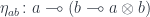
A Tambara module (a.k.a., a strong profunctor) is a profunctor equipped with the following mapping:

$\alpha_{a b c} \colon p a b \to p (c \otimes a) (c \otimes b)$

natural in $a$ and $b$ , dintural in $c$ .
In Haskell, this translates to a polymorphic function:

class (Profunctor p) => Tambara p where
   alpha :: forall a b c. p a b -> p (c, a) (c, b)

The linear lens $L a b s t$ is itself a Tambara module, for fixed $a b$ . To show this, let’s construct a mapping:

$\alpha_{s t c} \colon L a b s t \to L a b (c \otimes s) (c \otimes t)$

Expanding the definition:

$\int^{c''} (s \multimap c'' \otimes a)\times (c'' \otimes b \multimap t) \to$
$\; \int^{c' } (c \otimes s \multimap c' \otimes a)\times (c' \otimes b \multimap c \otimes t)$

By cocontinuity of the hom-set in $\mathbf{Set}$ , a mapping out of a coend is equivalent to an end:

$\int_{c''} \Big( (s \multimap c'' \otimes a)\times (c'' \otimes b \multimap t) \to$
$\;\int^{c' } (c \otimes s \multimap c' \otimes a)\times (c' \otimes b \multimap c \otimes t) \Big)$

Given a pair of linear arrows on the left we want to construct a coend on the right. We can do it by first lifting both arrow by $(c \otimes -)$ . We get:

$(c \otimes s \multimap c \otimes c'' \otimes a)\times (c \otimes c'' \otimes b \multimap c \otimes t)$

We can inject them into the coend on the right at $c' = c \otimes c''$ .

In Haskell, we construct the instance of the Profunctor class for the linear lens:

instance Profunctor (LinLensEx a b) where
  dimap f' g' (LinLensEx f g) = LinLensEx (f . f') (g' . g)

and the instance of Tambara:

instance Tambara (LinLensEx a b) where
  alpha (LinLensEx f g) = 
    LinLensEx (unassoc . second f) (second g . assoc)

Linear lenses can be composed and there is an identity linear lens:

$id_{a b} \colon L a b a b = \int^c (a \multimap c \otimes a)\times (c \otimes b \multimap b)$

given by injecting the pair $(id_a, id_b)$ at $c = I$ , the monoidal unit.

In Haskell, we can construct the identity lens using the left unitor (see Appendix 1):

idLens :: LinLensEx a b a b
idLens = LinLensEx unlunit lunit

The profunctor representation of a linear lens is given by an end over Tambara modules:

$L a b s t \cong \int_{p : Tamb} p a b \to p s t$

In Haskell, this translates to a type of functions polymorphic in Tambara modules:

type PLens a b s t = forall p. Tambara p => p a b -> p s t

The advantage of this representation is that it lets us compose linear lenses using simple function composition.

Here’s the categorical proof of the equivalence. Left to right: Given a triple: $(c, f \colon s \multimap c \otimes a, g \colon c \otimes b \multimap t)$ , we construct:

$p a b \xrightarrow{\alpha_{a b c}} p (c \otimes a) (c \otimes b) \xrightarrow{p f g} p s t$

Conversely, given a polymorphic (in Tambara modules) function $p a b \to p s t$ , we can apply it to the identity optic $id_{a b}$ and obtain $L a b s t$ .

In Haskell, this equivalence is witnessed by the following pair of functions:

fromPLens :: PLens a b s t -> LinLensEx a b s t
fromPLens f = f idLens

toPLens :: LinLensEx a b s t -> PLens a b s t
toPLens (LinLensEx f g) pab = dimap f g (alpha pab)

van Laarhoven representation

Similar to regular lenses, linear lenses have a functor-polymorphic van Laarhoven encoding. The difference is that we have to use endofunctors in the monoidal subcategory, where all arrows are linear:

class Functor f where
  fmap :: (a %1-> b) %1-> f a %1-> f b

Just like regular Haskell functors, linear functors are strong. We define strength as:

strength :: Functor f => (a, f b) %1-> f (a, b)
strength (a, fb) = fmap (eta a) fb

where eta is the unit of the currying adjunction (see Appendix 1).

With this definition, the van Laarhoven encoding of linear lenses is:

type VLL s t a b = forall f. Functor f => 
    (a %1-> f b) -> (s %1-> f t)

The equivalence of the two encodings is witnessed by a pair of functions:

toVLL :: LinLens s t a b -> VLL s t a b
toVLL lns f = fmap apply . strength . second f . lns

fromVLL :: forall s t a b. VLL s t a b -> LinLens s t a b
fromVLL vll s = unF (vll (F id) s)

Here, the functor F is defined as a linear pair (a tensor product):

data F a b x where
   F :: (b %1-> x) %1-> a %1-> F a b x
unF :: F a b x %1-> (b %1-> x, a)
unF (F bx a) = (bx, a)

with the obvious implementation of fmap

instance Functor (F a b) where
  fmap f (F bx a) = F (f . bx) a

You can find the categorical derivation of van Laarhoven representation in Appendix 2.

Linear optics

Linear lenses are but one example of more general linear optics. Linear optics are defined by the action of a monoidal category $\mathcal M$ on (possibly the same) monoidal category $\mathcal C$ :

$\bullet \colon \mathcal M \times \mathcal C \to \mathcal C$

In particular, one can define linear prisms and linear traversals using actions by a coproduct or a power series.

The existential form is given by:

$O a b s t = \int^{m \colon \mathcal M} (s \multimap m \bullet a)\times (m \bullet b \multimap t)$

There is a corresponding Tambara representation, with the following Tambara structure:

$\alpha_{a b m} \colon p a b \to p (m \bullet a) (m \bullet b)$

Incidentally, the two hom-sets in the definition of the optic can come from two different categories, so it’s possible to mix linear and non-linear arrows in one optic.

Appendix: 1 Closed monoidal category in Haskell

With the advent of linear types we now have two main categories lurking inside Haskell. They have the same objects–Haskell types– but the monoidal category has fewer arrows. These are the linear arrows $a \multimap b$ . They can be composed:

(.) :: (b %1-> c) %1-> (a %1-> b) %1-> a %1 -> c
(f . g) x = f (g x)

and there is an identity arrow for every object:

id :: a %1-> a
id a = a

In general, a tensor product in a monoidal category is a bifunctor: $\mathcal C \times \mathcal C \to \mathcal C$ . In Haskell, we identify the tensor product $\otimes$ with the built-in product (a, b). The difference is that, within the monoidal category, this product doesn’t have projections. There is no linear arrow $(a, b) \multimap a$ or $(a, b) \multimap b$ . Consequently, there is no diagonal map $a \multimap (a, a)$ , and the unit object $()$ is not terminal: there is no arrow $a \multimap ()$ .

We define the action of a bifunctor on a pair of linear arrows entirely within the monoidal category:

class Bifunctor p where
    bimap :: (a %1-> a') %1-> (b %1-> b') %1-> 
             p a b %1-> p a' b'
    first :: (a %1-> a') %1-> p a b %1-> p a' b
    first f = bimap f id
    second :: (b %1-> b') %1-> p a b %1-> p a b'
    second = bimap id

The product is itself an instance of this linear bifunctor:

instance Bifunctor (,) where
    bimap f g (a, b) = (f a, g b)

The tensor product has to satisfy coherence conditions–associativity and unit laws:

assoc :: ((a, b), c) %1-> (a, (b, c))
assoc ((a, b), c) = (a, (b, c))
unassoc :: (a, (b, c)) %1-> ((a, b), c)
unassoc (a, (b, c)) = ((a, b), c)

lunit :: ((), a) %1-> a
lunit ((), a) = a
unlunit :: a %1-> ((), a)
unlunit a = ((), a)

In Haskell, the type of arrows between any two objects is also an object. A category in which this is true is called closed. This identification is the consequence of the currying adjunction between the product and the function type. In a closed monoidal category, there is a corresponding adjunction between the tensor product and the object of linear arrows. The mapping out of a tensor product is equivalent to the mapping into the function object. In Haskell, this is witnessed by a pair of mappings:

curry :: ((a, b) %1-> c) %1-> (a %1-> (b %1-> c))
curry f x y = f (x, y)

uncurry :: (a %1-> (b %1-> c)) %1-> ((a, b) %1-> c)
uncurry f (x, y) = f x y

Every adjunction also defines a pair of unit and counit natural transformations:

eta :: a %1-> b %1-> (a, b)
eta a b = (a, b)

apply :: (a %1-> b, a) %-> b
apply (f, a) = f a

We can, for instance, use the unit to implement a point-free mapping of lenses:

toLinLens :: LinLensEx a b s t -> LinLens s t a b
toLinLens (LinLensEx f g) = first ((g .) . eta) . f

Finally, a note about the Haskell definition of a profunctor:

class Profunctor p where
  dimap :: (a' %1-> a) -> (b %1-> b') -> p a b -> p a' b'

Notice the mixing of two types of arrows. This is because a profunctor is defined as a mapping $\mathcal C^{op} \times \mathcal C \to \mathbf{Set}$ . Here, $\mathcal C$ is the monoidal category, so the arrows in it are linear. But p a b is just a set, and the mapping p a b -> p a' b' is just a regular function. Similarly, the type:

 (a' %1-> a)

is not treated as an object in $\mathcal C$ but rather as a set of linear arrows. In fact this hom-set is itself a profunctor:

newtype Hom a b = Hom (a %1-> b)

instance Profunctor Hom where
  dimap f g (Hom h) = Hom (g . h . f)

As you might have noticed, there are many definitions that extend the usual Haskel concepts to linear types. Since it makes no sense to re-introduce, and give new names to each of them, the linear extensions are written using multiplicity polymorphism. For instance, the most general currying function is written as:

curry :: ((a, b) %p -> c) %q -> a %p -> b %p -> c

covering four different combinations of multiplicities.

Appendix 2: van Laarhoven representation

We start by defining functorial strength in a monoidal category:

$\sigma_{a b} \colon a \otimes F b \multimap F (a \otimes b)$

To begin with, we can curry $\sigma$ . Thus we have to construct:

$a \multimap (F b \multimap F (a \otimes b))$

We have at our disposal the counit of the currying adjunction:

$\eta_{a b} \colon a \multimap (b \multimap a \otimes b)$

We can apply $\eta_{a b}$ to $a$ and lift the resulting map $(b \multimap a \otimes b)$ to arrive at $F b \multimap F (a \otimes b)$ .

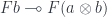Now let’s write the van Laarhoven representation as the end of the mapping of two linear hom-sets:

$\int_{F \colon [\mathcal C, \mathcal C]} (a \multimap F b) \to (s \multimap F t)$

We use the Yoneda lemma to replace $a \multimap F b$ with a set of natural transformations, written as an end over $x$ :

$\int_{F} \int_x \big( (b \multimap x) \multimap (a \multimap F x)\big) \to (s \multimap F t)$

We can uncurry it:

$\int_{F} \int_x \big( (b \multimap x) \otimes a \multimap F x \big) \to (s \multimap F t)$

and apply the ninja-Yoneda lemma in the functor category to get:

$s \multimap ((b \multimap t) \otimes a)$

Here, the ninja-Yoneda lemma operates on higher-order functors, such as 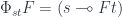$\Phi_{s t} F = (s \multimap F t)$ . It can be written as:

$\int_{F} \int_x (Gx \multimap Fx) \to \Phi_{s t} F \cong \Phi_{s t} G$

Appendix 3: My resource management curriculum

These are some of my blog posts and articles about resource management and its application to concurrent programming.

Strong Pointers and Resource Management in C++,
- Part 1, 1999
- Part 2, 2000
Walking Down Memory Lane, 2005 (with Andrei Alexandrescu)
unique ptr–How Unique is it?, 2009
Unique Objects, 2009
Race-free Multithreading, 2009
- Part 1: Ownership
- Part 2: Owner Polymorphism
Edward C++ hands, 2013

Bartosz Milewski's Programming Cafe

Sieves and Sheaves

Covering Sieves

Sheaves as Virtual Objects

Linear Lenses in Haskell

Linear types

Linear lens: The existential form

Profunctor representation

van Laarhoven representation

Linear optics

Appendix: 1 Closed monoidal category in Haskell

Appendix 2: van Laarhoven representation

Appendix 3: My resource management curriculum

Top Posts

License

Blogroll

Follow Me

Archives