Homotopy | Bartosz Milewski's Programming Cafe

October 18, 2025

Modeling Identity Types

Previously: Identity Types.

Let me first explain why the naive categorical model of dependent types doesn’t work very well for identity types. The problem is that, in such a model, any arrow can be considered a fibration, and therefore interpreted as a dependent type. In our definition of path induction, with an arrow $d$ that makes the outer square commute, there are no additional constraints on $\rho$ :

So we are free to substitute $\text{refl} \colon A \to \text{Id}_A$ for $\rho$ , and use the identity for $d$ :

We are guaranteed that there is a unique $J$ that makes the two triangles commute. But these commutation conditions tell us that $J$ is the inverse of $\text{refl}$ and, consequently, $\text{Id}_A$ is isomorphic to $A$ . It means that there are no paths in $\text{Id}_A$ other than those given by reflexivity.

This is not satisfactory from the point of homotopy type theory, since the existence of non-trivial paths is necessary to make sense of things like higher inductive types (HITs) or univalence. If we want to model dependent types as fibrations, we cannot allow $\text{refl}$ to be a fibration. Thus we need a more restrictive model in which not all mappings are fibrations.

The solution is to apply the lessons from topology, in particular homotopy. Recall that maps between topological spaces can be characterized as fibrations, cofibrations, and homotopy equivalences. There usually are overlaps between these three categories.

A fibration that is also an equivalence is called a trivial fibration or an acyclic fibration. Similarly, we have trivial (acyclic) cofibrations. We’ve also seen that, roughly speaking, cofibrations generalize injections. So, if we want a non-trivial model of identity types, it makes sense to model $\text{refl}$ as a cofibration. We want different values $a \colon A$ to be mapped to different “paths” $\text{refl}(a) \colon \text{Id}_A$ , and we’d also like to have some non-trivial paths left over to play with.

We know what a path is in a topological space $A$ : it’s a continuous mapping from a unit interval, $\gamma \colon I \to A$ . In a cartesian category with weak equivalences, we can use an abstract definition of the object representing the space of all paths in $A$ . A path space object $P_A$ is an object that factorizes the diagonal morphism $\Delta = \pi \circ s$ , such that $s$ is a weak equivalence.

In a category that supports a factorization system, we can tighten this definition by requiring that $\pi$ be a fibration, defining a good path object; and $s$ be a cofibration (therefore a trivial cofibration) defining a very good path object.

The intuition behind this diagram is that $\pi$ produces the start and the end of a path, and $s$ sends a point to a constant path.

Compare this with the diagram that illustrates the introduction rule for the identity type:

We want $\text{refl}$ to be a trivial cofibration, that is a cofibration that’s a weak homotopy equivalence. Weak equivalence let us shrink all paths. Imagine a path as a rubber band. We fix one end and of the path and let the other end slide all the way back until the path becomes constant. (In the compact/open topology of $P_A$ , this works also for closed loops.)

Thus the existence of very good path objects takes care of the introduction rule for identity types.

The elimination rule is harder to wrap our minds around. How is it possible that any mapping that is defined on trivial paths, which are given by $\text{refl}$ over the diagonal of $A \times A$ , can be uniquely extended to all paths?

We might take a hint from complex analysis, where we can uniquely define analytic continuations of real function.

In topology, our continuations are restricted by continuity. When you are lifting a path in $A$ , you might not have much choice as to which value of type $D(a)$ to pick next. In fact, there might be only one value available to you — the “closest one” in the direction you’re going. To choose any other value, you’d have to “jump,” which would break continuity.

You can visualize building $J(a, b, p)$ by growing it from its initial value $J(a, a, \text{refl}(a)) = d(a)$ . You gradually extend it above the path $p$ until you reach the point directly above $b$ . (In fact, this is the rough idea behind cubical type theory.)

A more abstract way of putting it is that identity types are path spaces in some factorization system, and dependent types over them are fibrations that satisfy the lifting property. Any path from $a$ to $b$ in $\text{Id}_A$ has a unique lifting $J$ in $D$ that starts at $d(a)$ .

This is exactly the property illustrated by the lifting diaram, in which paths are elements of the identity type $\text{Id}_A$ :

This time $\text{refl}$ is not a fibration.

The general framework, in which to build models of homotopy type theory is called a Quillen model category, which was originally used to model homotopies in topological spaces. It can be described as a weak factorization system, in which any morphism can be written as a trivial cofibration followed by a fibration. It must satisfy the unique lifting property for any square in which $i$ is a cofibration, $p$ is a fibration, and one of them is a weak equivalence:

The full definition of a model category has more moving parts, but this is the gist of it.

We model dependent types as fibrations in a model category. We construct path objects as factorizations of the diagonal, and this lets us define non-trivial identity types.

One of the consequences of the fact that there could be multiple identity paths between two points is that we can, in turn, compare these paths for equality. There is, for instance, an identity type of identity types $\text{Id}_{\text{Id}_A(a, b)}$ . Such iterated types correspond to higher homotopies: paths between paths, and so on, ad infinitum. The structure that arises is called a weak infinity groupoid. It’s a category in which every morphism has an inverse (just follow the same path backwards), and category laws (identity or associativity) are satisifed up to higher morphisms (higher homotopies).

September 22, 2025

Identity Types

Posted by Bartosz Milewski under Category Theory, Homotopy, Homotopy Type Theory | Tags: Category Theory, Homotopy, HoTT, Identity Type |
[2] Comments

Previously: Models of (Dependent) Type Theory.

There is a deep connection between mathematics and programming. Computer programs deal with such mathematical objects as numbers, vectors, monoids, functors, algebras, and many more. We can implement such structures in most programming languages. For instance, here’s the definition of natural numbers in Haskell:

data Nat where
  Z :: Nat           -- zero
  S :: Nat -> Nat    -- successor

There is a problem, though, with encoding the laws that they are supposed to obey. These laws are expressed using equalities. But not all equalities are created equal. Take, for instance, this definition of addition:

plus :: Nat -> Nat -> Nat
plus Z n = n
plus (S n) m = S (plus n m)

The first clause tells us that $0 + n$ is equal to $n$ . This is called definitional equality, since it’s just part of the definition. However, if we reverse the order of the addends and try to prove $n + 0 = n$ , there is no obvious shortcut. We have to prove it the hard way! This second type of equality is called propositional.

In traditional mathematics equality is treated as a relation. Two things are either equal or not. In type theory, on the other hand, equality is a type. It’s a type of proofs of equality. When you postulate that two things are equal, you specify the type of proofs that you are willing to accept.

Equality is a dependent type, because it depends on the values that are being compared. For a pair of values of the type $A$ , the identity (or equality) type is denoted by $\text{Id}_A$ :

$\frac{a, b \colon A}{\text{Id}_A (a, b) \colon \text{Type}}$

(In this notation, assumptions are listed above the horizontal line.)

You’ll also see $\text{Id}_A(a, b)$ written as $a =_A b$ , or even $a = b$ , if the type $A$ is obvious from the context.

When two values are not equal, this type is uninhabited. Otherwise it’s inhabited by proofs, or witnesses, of equality. This is consistent with the propositions as types interpretation of type theory.

For the identity type to be useful, we have to have a way to populate it with values — proofs of equality. We do that by providing an introduction rule:

$\frac{a \colon A}{\text{refl}(a) \colon \text{Id}_A(a, a)}$

The constructor $\text{refl}$ generates a witness to the obvious fact that, for every $a$ , $a = a$ . Here, $\text{refl}$ is the abbreviation of reflexivity.

At first sight it doesn’t seem like we have gained anything by turning equality into a type. Indeed, if $\text{refl}$ were the only inhabitant of $\text{Id}_A$ , we’d just buy ourselves a lot of headaches for nothing. The trouble is that, if there is a type $\text{Id}_A(a, b)$ , then there’s also a type $\text{Id}_{\text{Id}_A(a,b)}$ (type of equality of proofs of equality), and so on, ad infinitum. This used to be a bane of Martin Löf type theory, but it became a bounty for Homotopy Type Theory. So let’s imagine that the identity type may have non-trivial inhabitants. We’ll call these inhabitants paths. The trivial paths generated by $\text{refl}$ are degenerate do-nothing loops.

But first, let’s consider the identity elimination rule: the mapping out of the identity type. What data do we need to provide in order to define a function from a path $p \colon \text{Id}_A(x, y)$ to some type $D$ ? In full generality, $D$ should be a dependent type family parameterized by the path $p$ as well as its endpoints $x$ and $y$ :

$x, y \colon A, \; p \colon \text{Id}_A (x, y) \vdash D(x, y, p) \colon \text{Type}$

Our goal is to define a $D$ -valued mapping $J$ that works for any path in $A$ :

$x, y \colon A, \; p \colon \text{Id}_A(x, y) \vdash J(x, y, p) \colon D(x, y, p)$

The trick is to realize that there is only one family of constructors of the identity type, $\text{refl}(a)$ , so it’s enough to specify how $J$ is supposed to act on it. We do this by providing a dependent function $d$ (a dependent function is a function whose return type depends on the value of its argument):

$a \colon A \vdash d(a) \colon D(a, a, \text{refl}(a))$

This is very similar to constructing a mapping out of a Boolean by specifying its action on the two constructors, $\text{True}$ and $\text{False}$ . Except that here we have a whole family of constructors $\text{refl}(a)$ parameterized by $a$ .

This is enough information to uniquely determine the action of $J$ on any path, provided it agrees with $d$ along $\text{refl}$ :

$J(a, a, \text{refl}(a)) = d(a)$

This procedure for defining mappings out of identity types is called path induction.

Categorical Model

We’ll build a categorical interpretation of identity types making as few assumptions as possible. We’ll model $\text{Id}_A$ as a fibration:

$\text{Id}_A \xrightarrow{\pi} A \times A$

The introduction rule asserts the existence of the arrow:

$A \xrightarrow{\text{refl}} \text{Id}_A$

For any given $a \colon A$ , this arrow selects a diagonal element of the identity type, $\text{Id}_A(a, a)$ . When projected down to $A \times A$ using $\pi$ , it lands on the diagonal of $A \times A$ . In a cartesian category, the diagonal is defined by the arrow $\Delta \colon A \to A \times A$ , so we have:

$\Delta = \pi \circ \text{refl}$

In other words, there is a factorization of the diagonal arrow.

The elimination rule starts with defining a dependent type $D$ , which can be modeled as a fibration $\rho$ :

$D \xrightarrow{\rho} \text{Id} \xrightarrow{\pi} A \times A$

We provide a dependent function $d$ , which is interpreted as an arrow $d : A \to D$ that maps $a$ to an element $d(a)$ of $D(a, a, \text{refl}(a))$ . So, when projected back to $\text{Id}_A$ using $\rho$ , it produces the same element as $\text{refl}(a)$

$\rho \circ d = \text{refl}$

Given these assumptions, there exists a mapping:

$x, y \colon A, p \colon \text{Id}_A(x, y) \vdash J(x, y, p) \colon D(x, y, p)$

which is interpreted as a section $\text{Id}_A \to D$ . The section condition is:

$\rho \circ J = id_{\text{Id}_A}$

This mapping is unique if we assume that it agrees with $d$ when restricted to $\text{refl}$ :

$J \circ \text{refl} = d$

Consequently, we can illustrate the path induction rule using a single commuting diagram:

If the outer square commutes then there is a unique diagonal arrow that makes the two triangles commute. The similarity to the lifting property of homotopy theory is not accidental, as we’ll see next.

Next: Modeling Identity Types.

July 26, 2025

(Weak) Factorization Systems

Posted by Bartosz Milewski under Homotopy, Topology | Tags: Homotopy, math, Topology |
Leave a Comment

Previously (Weak) Homotopy Equivalences.

An average function between sets, $f \colon A \to B$ is neither surjective nor injective. We can however isolate the two “failure modes” if we insert a third set $X$ in between. We can, for instance, pick this set to be the subset of $B$ that is the image of $A$ under $f$ . We then define $s \colon A \twoheadrightarrow X$ to be the surjective part of $f$ . This way $s$ deals just with all the non-injectivity of $f$ . We can then follow $s$ with an injective function $i \colon X \hookrightarrow B$ . We get the (Surj, Inj) factorization of an arbitrary function into a surjection followed by an injection:

$f = i \circ s$

This factorization is unique up to unique isomorphism.

Notice also that both surjections and injections are closed under composition and that every isomorphism is simultaneously a surjection and an injection.

In category theory we generalize this idea to define abstract factorization systems.

A (strict) factorization system specifies two classes of morphisms $L$ and $R$ , satisfying conditions loosely analogous to the (Surj, Inj) factorization:

Each class is closed under composition and contains all isomorphisms.
Every morphism can be factorized, $f = r \circ l$ , with $l \in L$ and $r \in R$
The factorization is functorial.

The last condition requires some explanation. We can look at factorization as a functor between two categories.

The source category is the arrow category of $C$ . Its objects are arrows or, more precisely, triples $(a, b, f \colon a \to b)$ . A morphism from $(a, b, f)$ to $(a', b', f')$ is a pair of arrows $(u \colon a \to a', v \colon b \to b')$ that make the following square commute:

The target category is the category of factorizations. Its objects are factorizations, or pairs of composable arrows $(l, r)$ :

$a \xrightarrow{l} x \xrightarrow{r} b$

taken from the two classes $(L, R)$ . Morphisms are triples of arrows $(u, w, v)$ that make the following diagram commute:

The functor in question maps an arrow $(a, b, f)$ to its factorization, $a \xrightarrow{l} x \xrightarrow{r} b$ , with $f = r \circ l$ . Its action on a morphism $(u, v)$ is the commuting diagram above. For functoriality, we need the arrow $w$ to be determined uniquely.

Notice that we can redraw the last diagram in such a way that $w$ crosses it diagonally.

In other words, morphisms in $L$ have the (strict) left lifting property with respect to morphisms in $R$ .

Interesting things start happening when we relax the strictness property and allow $w$ not to be unique. We can no longer talk about functoriality of factorization. Instead we lean on the (weak) lifting property.

To illustrate this, let’s reverse the roles of surjections and injections in our factorization of functions. Indeed, every function can be factored into an injection followed by a surjection. Such (Inj, Surj) factorization is not unique. (It also requires the use of the Axiom of Choice.)

A weak factorization system consists, as before, of two classes of morphisms $(L, R)$ that allow for factoriziation of an arbitrary morphism $f = l \circ r$ . This time, however, we postulate that $L$ is precisely the class of morphisms with a left lifting property against every morphism in $R$ ; and vice versa for $R$ and the right lifting property.

At this point you may recall the lifting property we discussed earlier between fibrations and cofibrations. In particular, a cofibration satisfies the homotopy extension property.

Interestingly, there is a connection between fibrations and surjections, and cofibrations and injections.

First, we’ll show that a fibration $p \colon E \to B$ is a surjection as long as $E$ is non empty and $B$ is path connected.

Here’s the proof: If $p$ were not surjective then there would be a point $b \in B$ that is not in the image of $p$ . Since $E$ is not empty, there exists a point $e \in E$ . Take any path $\gamma$ in $B$ connecting $p \, e$ to $b$ . Since $p$ is a fibration, we can lift this path to $\tilde{\gamma}$ in $E$ . Since $p$ projects the endpoint of $\tilde{\gamma}$ to $b$ , we have reached a contradiction. Therefore $p$ must be a surjection. $\blacksquare$

The proof that every cofibration is injective is a bit more involved. It uses a very handy notion of a mapping cylinder. We can visualize a function $i \colon B \to E$ between two spaces as a bunch of wires. Each wire connects a point $b \in B$ to the corresponding point $i \, b \in E$ . A mapping cylinder $M_i$ is a topological space that formalizes this picture.

We start with pairs $(b, t) \in B \times I$ , where $I$ is the unit segment, which we use to parameterize the length of each wire. Then we add the target $E$ to our cylinder, and plug the end $(b, 1)$ of each wire to its “socket” $i \, b \in E$ .

Formally, the mapping cylinder $M_i$ is a quotient space of the disjoint union $(B \times I) \bigsqcup E$ , identifying each $(b, 1)$ with $i \, b$ .

Notice that, if $i$ is not injective, there will be some merging of multiple wires right when they hit $E$ , but not earlier–the fact that will become relevant later.

Now let’s use the cofibration property of $i$ . We replace the big space $X$ with the cylinder $M_i$ . The arrow $e$ is the inclusion $e \colon E \hookrightarrow M_i$ . Notice that $e$ will be identified with the starting point of the homotopy $\tilde h_0$ that we’re constructing.

First we define the homotopy $h \colon B \times I \to M_i$ . For every $t \in I$ , we write $h_t \colon B \to M_i$ .

At $t = 0$ , $h_0\, b$ is the point in $M_i$ that sits on the seam between $B \times I$ and $E$ . In our quotient space, it corresponding to $i \, b$ .

For $t > 0$ we define $h_t \, b = \{(b, 1-t)\}$ . It reverses the direction of wires in the cylinder $M_i$ . (We use curly braces to embed the pair $(b, 1-t) \in B \times I$ into the quotient $M_i$ .)

The function $h$ is continuous, therefore a homotopy. (It may still merge multiple points into one, if $i$ is not injective.)

Cofibration condition states that any homotopy $h \colon B \times I \to M_i$ can be lifted to $\tilde h \colon E \times I \to M_i$ , such that $h (b, t) =\tilde h (i \, b, t)$ . The latter condition can be written as:

$h_t = \tilde h_t \circ i$

In our case, $\tilde h_0$ will shrink the whole of $E$ down to $i \, B$ before embedding it in $M_i$ .

Then, for any $t > 0$ , $\tilde h_t$ will shrink $E$ down to $B$ , embed it in $B \times I$ at $1 - t$ , and inject it into $M_i$ .

Notice that, for any fixed $t > 0$ , our $h_t$ is injective ( $h$ could only do the merging of wires at $t = 0$ , where the identification happens). But the lifting condition tells us that $h_t = \tilde h_t \circ i$ . Therefore $i$ must also be injective. $\blacksquare$

We have shown that fibrations between (path-connected, non-empty) topological spaces are surjective, and that cofibrations are injective.

Corresponding to the weak (Inj, Surj) factorization system in Set, we can build a weak (Cofib, Fib) factorization system in Top (the category of topological spaces). Indeed, under some conditions, every continuous function can be factored into a cofibration followed by a fibration.

We’ve seen earlier that cofibrations have the left lifting property with respect to fibrations, and vice versa. So (Cofib, Fib) is indeed an example of a weak factorization system. We’ll see later that weak factorization systems form the basis of Quillen model categories.

Next: Models of (Dependent) Type Theory.

June 20, 2025

(Weak) Homotopy Equivalences

Posted by Bartosz Milewski under Category Theory, Homotopy, Homotopy Type Theory, Topology | Tags: Category Theory, Homotopy, math, Topology |
Leave a Comment

Previously: Fibrations and Cofibrations.

In topology, we say that two shapes are the same if there is a homeomorphism– an invertible continuous map– between them. Continuity means that nothing is broken and nothing is glued together. This is how we can turn a coffe cup into a torus. A homeomorphism, however, won’t let us shrink a torus to a circle. So if we are only interested in how many holes the shapes have, we have to relax our notion of equivalence.

Let’s go back to the definition of homeomorphism. It is defined as a pair of continuous functions between two topological spaces, $f \colon X \to Y$ and $g \colon Y \to X$ , such that their compositions are identity maps, $f \circ g = id_Y$ and $g \circ f = id_X$ , respectively.

If we want to allow for extreme shrinkage, as with a (solid) torus shrinking down to a circle, we have to relax the identity conditions.

A homotopy equivalence is a pair of continuous functions, but their compositions don’t have to be equal to identities. It’s enough that they are homotopic to identities. In other words, it’s possible to create an animation that transforms one to another.

Take the example of a line $\mathbb R$ and a point. The point is a trivial topological space where only the whole space (here, the singleton $\{*\}$ ) and the empty set are open. $\mathbb R$ and $\{*\}$ are obviously not homeomorphic, but they don’t have any holes, so they should be homotopy equivalent.

Indeed, let’s construct the equivalence as a pair of constant functions: $f \colon x \mapsto *$ and $g \colon * \mapsto 0$ (the origin of $\mathbb R$ ). Both are continuous: The pre-image $f^{-1} \{ * \}$ is the whole real line, which is open. The pre-image $g^{-1}$ of any open set in $\mathbb R$ is $\{*\}$ , which is also open.

The composition $f \circ g \colon * \mapsto *$ is equal to the identity on $\{*\}$ , so it’s automatically homotopic to it. The interesting part is the composition $g \circ f \colon x \mapsto 0$ , which is emphatically not equal to identity on $\mathbb R$ . We can however construct a homotpy between the identity and it. It’s a function that interpolates between them:

$h \colon \mathbb R \times I \to \mathbb R$

$h (x, 0) = id_{\mathbb R} x = x$

$h(x, 1) = (g \circ f) x = 0$

( $I$ is the unit interval $[0, 1]$ .) Such a function exists:

$h (x, t) = (1 - t) \,x$

When a space is homotopy equivalent to a point, we say that it’s contractible. Thus $\mathbb R$ is contractible. Similarly, n-dimensional spaces, $\mathbb R^n$ , as well as n-dimensional balls are all contractible. A circle, however, is not contractible, because it has a hole.

Another way of looking for holes in spaces is by trying to shrink loops. If there is a hole inside a loop, it cannot be continuously shrunk to a point. Imagine a loop going around a circle. There is no way you can “unwind” it without breaking something. In fact, you can have loops that wind n times around a circle. They can’t be homotopied into each other if their winding numbers are different.

In general, paths in a topological space $X$ , i.e. continuous mappings $\gamma \colon I \to X$ , naturally split into equivalence classes with respect to homotopy. Two paths, $\gamma$ and $\gamma'$ , sharing the same endpoints are in the same class if there is a homotopy between them:

$h \colon I \times I \to X$

$h (0, t) = \gamma t$

$h (1, t) = \gamma' t$

Moreover, two paths can be composed, as long as the endpoint of one coincides with the start point of the other (after performing appropriate reparametrizations).

There is a unit of such composition, a constant path; and every path has its inverse, a path that traces the original but goes in the opposite direction.

It’s easy to see that path composition induces a groupoid structure on the set of equivalence classes of paths. A groupoid is a category in which every morphism (here, path) is invertible. This particular groupoid is called the fundamental groupoid of the topological space $X$ .

If we pick a base point $x_0$ in $X$ , the paths that start and end at this point form closed loops. These loops then form a fundamental group $\pi_1(X, x_0)$ .

Notice that, as long as there is a path $\gamma$ from $x_0$ to $x_1$ , the fundamental groups at both points are isomorphic. This is because every loop $l$ at $x_1$ induces a loop at $x_0$ given by the concatenation $l' = \gamma^{-1} \circ l \circ \gamma$ .

So there is essentially a single fundamental group for the whole space, as long as $X$ is path-connected, i.e., it doesn’t split into multiple disconnected chunks.

Going back to our example of a circle, its fundamental group is the group of integers $\mathbb Z$ with addition. All loops that wind n-times around the circle in one direction correspond to the integer n.

Negative integers correspond to loops winding in the opposite direction. If you follow an n-loop with an m-loop, you get an (m+n)-loop. Zero corresponds to loops that can be shrunk to a point.

To tie these two notions of hole-counting together, it can be shown that two spaces that are homotopy equivalent also have the same fundamental groups. This makes sense, since equivalent spaces have the same holes.

Not only that, they also have the same higher homotopy groups (as long as both are path-connected).

We define the n-th homotopy group by replacing simple loops (which are homotopic to a circle, or a 1-dimensional sphere) with n-dimensional spheres. Attempts at shrinking those may detect higher-dimensional holes.

For instance, imagine an Earth-like ball with it’s inner core scooped out. Any 1-loop inside its bulk can be shrunk to a point (it will glide off the core). But a 2-sphere that envelops the core cannot be shrunk.

In fact such a 2-sphere can be wrapped around the core an arbitrary number of times. In math notation, we say:

$\pi_2 (B^3 \setminus \{ 0 \}) = \mathbb Z$

Corresponding to these higher homotopy groups there is also a higher homotopy groupoid, in which there are invertible paths, surfaces between paths, volumes between surfaces, etc. Taken together, these form an infinity groupoid. It is exactly the inspiration behind the infinity groupoid in homotopy type theory, HoTT.

Spaces that are homotopy equivalent have the same homotopy groups, but the converse is not true. There are spaces that are not homotopy equivalent even though they have the same homotopy groups. This is why a weaker version of equivalence was introduced.

A map between topological spaces is called a weak homotopy equivalence if it induces isomorphisms between all homotopy groups.

There is a subtle difference between strong and weak equivalences. Strong equivalence can be broken by a local anomaly, like in the following example: Take $X = \{0, 1, 2, ... \}$ , the set of natural numbers in which every number is considered an open set. Take $Y = \{ 0 \} \cup \{ 1, \frac{1}{2}, \frac{1}{3}, ... \}$ with the topology inherited from the real line.

The singleton set $\{ 0 \}$ in $Y$ is the obstacle to constructing a homeomorphism or a homotopy equivalence between $X$ and $Y$ . That’s because it is not open (there is no open set in $\mathbb R$ that contains it and nothing else). However, it’s impossible to have a non-trivial loop that would contain it, so $X$ and $Y$ are weakly equivalent.

Grothendieck conjectured that the infinity groupoid captures all information about a topological space up to weak homotopy equivalence.

Weak equivalences, together with fibrations and cofibrations, form the foundation of weak factorization systems and Quillen model categories.
Next: (Weak) Factorization Systems.

May 30, 2025

Fibrations and Cofibrations

Posted by Bartosz Milewski under Category Theory, Homotopy, Homotopy Type Theory, Topology | Tags: Category Theory, Cofiber, Cofibration, Fibration, Homotopy, Topology |
1 Comment

Previously: Subfunctor Classifier.

We are used to thinking of a mapping as either being invertible or not. It’s a yes or no question. A mapping between sets is invertible if it’s both injective and surjective. It means that it never merges two elements into one, and it covers the whole target set.

But if you are willing to look closer, the failures of invertibility are a whole fascinating area of research. Things get a lot more interesting if you consider mapping between topological spaces, which have to skillfully navigate around various holes and tears in the target space, and shrink or glue together parts of the source space. I will be glossing over some of the topological considerations, concentrating on the big-picture intuitions (both culinary and cinematographic).

Fibrations

In what follows, we’ll be considering a function $p \colon E \to B$ . We’ll call $p$ a projection from the total set $E$ to the base set $B$ .

Let’s start by considering the first reason for a failure of invertibility: multiple elements being mapped into one. Even though we can’t invert such a mapping, we can use it to fibrate the source $E$ .

To each element $y \in B$ we’ll assign a fiber, the set of elements of $E$ that are mapped to $y$ . By abuse of notation, we call such a fiber $p^{-1} y$ :

$p^{-1} y = \{ x |\; p x = y \}$

For some $y$ ‘s, this set may be empty $\emptyset$ ; for others, it may contain lots elements.

Notice that $p$ is an isomorphism if and only if every fiber is a singleton set. This property gives rise to a very useful definition of equivalence in homotopy type theory, where we ask for every fiber to be contractible.

A set-theoretic union of all fibers reconstructs the total set $E$ .

Things get more interesting when we move to topological spaces and continuous functions. To begin with, we can define a path in $B$ as a continuous mapping from the unit interval $I = [0, 1]$ to $B$ .

$\gamma \colon I \to B$

We can then ask if it’s possible to lift this path to $E$ , that is to construct $\tilde{\gamma} \colon I \to E$ that lies above $\gamma$ . To do this, we pick the starting point $e \in E$ that lies above the starting point of $\gamma$ , that is $p \,e = \gamma \,0$ .

This setup can be summarized in the commuting square:

The lifting $\tilde{\gamma}$ is then the diagonal arrow that makes both triangles commute:

It’s helpful to imagine a path as a trajectory of a point moving through a topological space. The parameter $t \in I$ is then interpreted as time.

In homotopy theory we generalize this idea to the movement, or deformation, of arbitrary shapes, not just points.

If we describe such a shape as the image of some topological space $X$ , its deformation is a mapping $h \colon X \times I \to B$ . Such potentially “fat” paths are called homotopies. In particular, if we replace $X$ by a single point, we recover our “thin” paths.

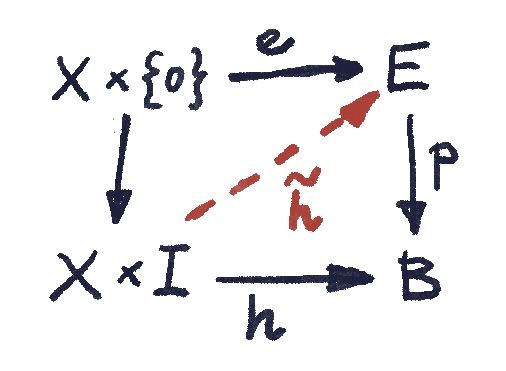
A homotopy lifting property is expressed as the existence of the diagonal function $\tilde h$ in this commuting square, such that the resulting triangles commute:

In other words, given a homotopy $h$ of the shape $X$ in the base, and an embedding $e$ of this shape in $E$ above $h \, 0$ , we can construct a homotopy in $E$ whose projection is $h$ .

Cofibrations

In category theory, every construction has its dual, which is obtained by reversing all the arrows. In topology, there is an analogous relation called the Eckmann-Hilton duality. Besides reversing the arrows, it also dualizes products to exponentials (using the currying adjunction), and injections to surjections.

When dualizing the homotopy lifting diagram, we replace the trivial injection of $X \times \{0\} \cong X$ into $X \times I$ by a surjection $\varepsilon_0$ of the exponential $X^I$ onto $X$ . Here, $X^I$ is the set of functions $I \to X$ , or the path space of $X$ . The surjection $\varepsilon_0$ maps every path $\gamma \colon I \to X$ to its starting point by evaluating it at zero. (The evaluation map $\varepsilon_t \colon \gamma \mapsto \gamma \,t$ is continuous in the compact-open topology of $X^I$ .)

The homotopy lifting property is thus dualized to the homotopy extension property:

Corresponding to the fibration that deals with the failure of the injectivity of $p$ , the homotopy extension property deals with the failure of the surjectivity of $i$ .

If the mapping $i$ has the extension property for all topological spaces $X$ , it is called a cofibration.

Intuitively, a cofibration is an embedding of $B$ in $E$ such that any “spaghettification” of $B$ , that is embedding it in the path space $X^I$ , can be extended to a spaghettification of $E$ . $X$ plays the role of an ambient space where these operations can be visualized. Later we’ll see how to construct a minimal such ambient space called a mapping cylinder.

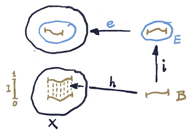
Let’s deconstruct the meaning of the outer commuting square.

$i$ embeds $B$ into $E$ .
$e$ further embeds $E$ into $X$ , and we end up with the embedding of $B$ inside $X$ given by $e \circ i$ .
$h$ embeds $B$ into the path space of $X$ (the dotted paths below).

The commuting condition for this square means that the starting points of all these paths, the result of applying $\varepsilon_0$ to each of them, coincide with the embedding of $B$ into $X$ given by $e \circ i$ . It’s like extruding a bunch of spaghetti, each strand corresponding to a point in $B$ .

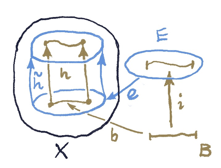
With this setup, we postulate the existence of the diagonal mapping $\tilde h \colon E \to X^I$ that makes the two triangles commute. In other words, $E$ is mapped to a family of paths in $X$ which, when restricted to the image of $B$ coincide with the original mapping $h$ .

The spaghetti extruded through the $E$ shape contain the spaghetti extruded through the $B$ shape.

Another intuitive description of this situation uses the idea of homotopy as animation. The strands of spaghetti become trajectories of particles.

We start by setting up the initial scene. We embed $E$ in the big space $X$ using $e \colon E \to X$ .

We have the embedding $i \colon B \to E$ , which induces the embedding of $B$ into $X$ :

$b = e \circ i$

Then we animate the embedding of $B$ using the homotopy

$h \colon B \times I \to X$

The initial frame of this animation is given by $b$ :

$h(x, 0) = b \, x$

We say that $i$ is a cofibration if every such animation can be extended to the bigger animation:

$\tilde h \colon E \times I \to X$

whose starting frame is given by $e$ :

$\tilde h (x, 0) = e \, x$ .

The commuting condition (for the lower triangle) means that the two animations coincide for all $x \in B$ and $t \in I$ :

$h (x, t) = \tilde h (i \,x, t)$

Just like a fiber is an epitome of non-injectiveness, one can define a cofiber as an epitome of non-surjectiveness. It’s essentially the part of $E$ that is not covered by $i$ .

As a topological space it’s the result of shrinking the image of $B$ inside $E$ to a point (the resulting topology is called the quotient topology).

Notice that, unlike with fibers, there is just one cofiber for a given cofibration (up to homotopy equivalence).

Lifting Property

A category theorist looking at the two diagrams that define, respectively, homotopy lifting and extension, will immediately ignore all the superfluous details. She will turn the second diagram upside down and merge it with the first diagram to get:

This is how we read the new diagram: If for any morphisms $f$ and $g$ that make the outer square commute, there exist a diagonal morphism $h$ that makes the two triangles commute, then we say that $i$ has the left lifting property with respect to $p$ . Equivalently, $p$ has the right lifting property with respect to $i$ .

Or we can say that the two morphisms are orthogonal to each other.

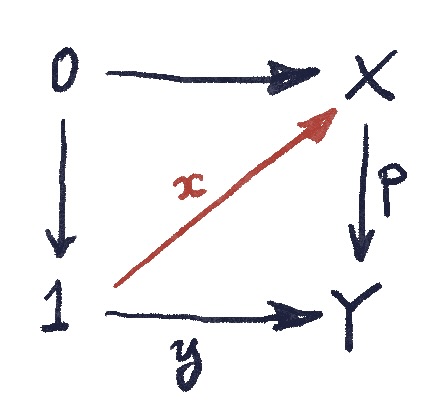
The motivation for this nomenclature is interesting. In the category of sets, the archetypal non-surjective function is the “absurd” $0 \to 1$ (or, in set notation, $\emptyset \to \{*\}$ ). It turns out that all surjective functions are its right liftings. In other words, all surjections are right-orthogonal to the simplest non-surjective function.

Indeed, the function at the bottom $y \colon 1 \to Y$ picks an element $y \in Y$ . Similarly, the diagonal function picks an element $x \in X$ . The commuting triangle tells us that for every $y$ there exists an $x$ such that $y = p \, x$ .

Similarly, we can show that all injective functions are orthogonal to the archetypal non-injective function $2 \to 1$ (or $\{x_1, x_2\} \to \{*\}$ ).

Indeed, assume that $i$ maps two different elements $a_1, a_2 \in A$ to a single element $b \in B$ . We could then pick $f$ such that $f \, a_1 = x_1$ and $f \, a_2 = x_2$ . The diagonal $h$ can map $b$ to either $x1$ or $x2$ but not both, so we couldn’t make the upper triangle commute.