March | 2025 | Bartosz Milewski's Programming Cafe

Proviously Sieves and Sheaves.

We have seen how topology can be defined by working with sets of continuous functions over coverages. Categorically speaking, a coverage is a special case of a sieve, which is defined as a subfunctor of the hom-functor $C(-, a)$ .

We’d like to characterize the relationship between a functor and its subfunctor by looking at them as objects in the category of presheaves. For that we need to introduce the idea of a subobject.

We’ll start by defining subobjects in the category of sets in a way that avoids talking about elements. Here we have two options.

The first one uses a characteristic function. It’s a predicate that answers the question: Is some element $x$ a member of a given subset or not? Notice that any Boolean-valued function uniquely defines a subset of its domain, so we don’t really need to talk about elements, just a function.

But we still have to define a Boolean set. Let’s call this set $\Omega$ , and designate one of its element as “True.” Selecting “True” can be done by defining a function $true \colon 1 \to \Omega$ , where $1$ is the terminal object (here, a singleton set). In principle we should insist that $\Omega$ contains two elements, “True” and “False,” but that would make it more difficult to generalize.

The second way to define a subset $S \subseteq P$ is to provide an injective function $m \colon S \rightarrowtail P$ that embeds $S$ in $P$ . Injectivity guarantees that no two elements are mapped to the same element. The image of $m$ then defines the subset of $P$ . In a general category, injective functions are replaced by monics (monomorphisms).

Notice that there can be many injections that define the same subset. It’s okay for them to permute the image of $m$ as long as it covers exactly the same subset of $P$ . (These injections form an equivalence class.)

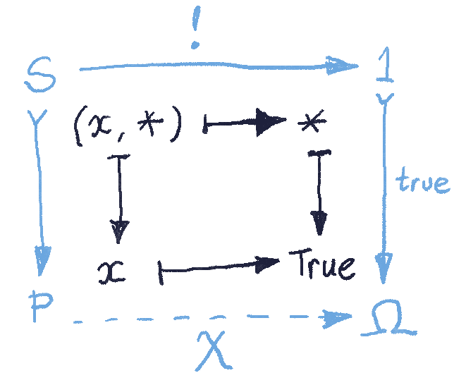
The fact that the two definitions coincide can be summarized by one commuting diagram. In the category of sets, given a characteristic function $\chi$ , the subset $S$ and the monic $m$ are uniquely (up to isomorphism) defined as a pullback of this diagram.

We can now turn the tables and use this diagram to define the object $\Omega$ called the subobject classifier, together with the monic $true \colon 1 \rightarrowtail \Omega$ . We do it by means of a universal construction. We postulate that: For every monic $S \rightarrowtail P$ between two arbitrary objects there exist a unique arrow $\chi \colon P \to \Omega$ such that the above diagram constitutes a pullback.

This is a slightly unusual definition. Normally we think of a pullback as defining the northwest part of the diagram given its southeast part. Here, we are solving a sudoku puzzle, trying to fill the southeast part to uniquely complete a pullback diagram.

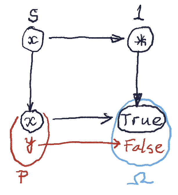
Let’s see how this works for sets. To construct a pullback (a.k.a., a fibered product $P \times_{\Omega} 1$ ) we first create a set of pairs $(x, *)$ where $x \in P$ and $* \in 1$ (the only element of the singleton set). But not all $x$ ‘s are acceptable, because we have a pullback condition, which says that $\chi x = \text{True}$ , where $\text{True}$ is the element of $\Omega$ pointed to by $true$ . This tells us that $S$ is isomorphic to the subset of $P$ for which $\chi$ is $\text{True}$ .

The question is: What happens to the other elements of $P$ ? They cannot be mapped to $\text{True}$ , so $\Omega$ must contain at least one more element (in case $m$ is not an isomorphism). Can it contain more?

This is where the universal construction comes into play. Any monic $m$ (here, an injective function) must uniquely determine a $\chi$ that completes the pullback. In particular, we can pick $S$ to be a singleton set and $P$ to be a two-element set. We see that if $\Omega$ contained only $\text{True}$ and nothing else, no $\chi$ would complete the pullback. And if $\Omega$ contained more than two elements, there would be not one but at least two such $\chi$ ‘s. So, by the Goldilock principle, $\Omega$ must have exactly two elements.

We’ll see later that this is not necessarily true in a more general category.

Next: Subfunctor Classifier.

There are many excellent AI papers and tutorials that explain the attention pattern in Large Language Models. But this essentially simple pattern is often obscured by implementation details and optimizations. In this post I will try to cut to the essentials.

In a nutshell, the attention machinery tries to get at a meaning of a word (more precisely, a token). This should be easy in principle: we could just look it up in the dictionary. For instance, the word “triskaidekaphobia” means “extreme superstition regarding the number thirteen.” Simple enough. But consider the question: What does “it” mean in the sentence “look it up in the dictionary”? You could look up the word “it” in the dictionary, but that wouldn’t help much. More ofthen than not, we guess the meaning of words from their context, sometimes based on a whole conversation.

The attention mechanism is a way to train a language model to be able to derive a meaning of a word from its context.

The first step is the rough encoding of words (tokens) as multi-dimensional vectors. We’re talking about 12,288 dimensions for GPT-3. That’s an enormous semantic space. It means that you can adjust the meaning of a word by nudging it in thousands of different directions by varying amounts (usually 32-bit floating point numbers). This “nudging” is like adding little footnotes to a word, explaining what was its precise meaning in a particular situation.

(Note: In practice, working with such huge vectors would be prohibitively expensive, so they are split between multiple heads of attention and processed in parallel. For instance, GPT-3 has 96 heads of attention, and each head works within a 128-dimensional vector space.)

We are embedding the input word as a 12,288-dimensional vector $\vec E$ , and we are embedding $N$ words of context as 12,288-dimensional vectors, $\vec E_i$ , $i = 1..N$ (for GPT-3, $N=2048$ tokens). Initially, the mapping from words to embeddings is purely random, but as the training progresses, it is gradually refined using backpropagation.

(Note: In most descriptions, you’ll see a whole batch of words begin embedded all at once, and the context often being identical with that same batch–but this is just an optimization.)

The goal is to refine the embedding $\vec E$ by adding to it a small delta $\Delta \vec E$ that is derived from the context $\vec E_i$ .

This is usually described as the vector $\vec E$ querying the context, and the context responding to this query.

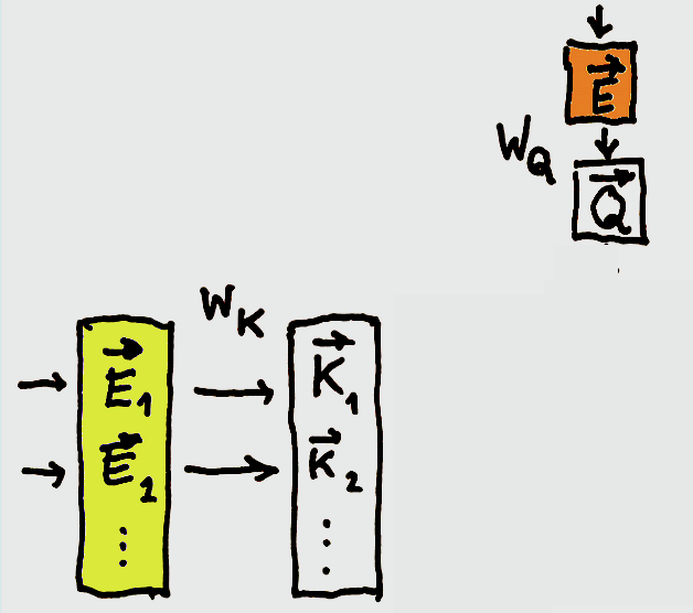
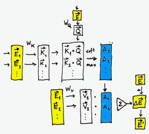
First, we apply a gigantic trainable 12,288 by 12,288 matrix $W_Q$ to the embedding $\vec E$ , to get the query vector:

$\vec Q = W_Q \vec E$

You may think of $\vec Q$ as the question: “Who am I with respect to the Universe?” The entries in the matrix $W_Q$ are the weights that are learned by running the usual backpropagation.

We then apply another trainable matrix $W_K$ to every vector $\vec E_i$ of the context to get a batch of key vectors:

$\vec K_i = W_K \vec E_i$

You may think of $\vec K_i$ as a possible response from the $i$ ‘th component of the context to all kinds of questions.

The next step is crucial: We calculate how relevant each element of the context is to our word. In other words, we are focusing our attention on particular elements of the context. We do it by taking $N$ scalar products $\vec K_i \cdot \vec Q$ .

A scalar product can vary widely. A large positive number means that the $i$ ‘th element of the context is highly relevant to the meaning of $\vec E$ . A large negative number, on the other hand, means that it has very little to contribute.

What we really need is to normalize these numbers to a range between zero (not relevant) and one (extremely relevant) and make sure that they all add up to one. This is normally done using the softmax procedure: we first raise $e$ to the power of the given number to make the result non-negative:

$a_i = exp (\vec K_i \cdot \vec Q)$

We then divide it by the total sum, to normalize it:

$A_i = \dfrac {a_i}{ \sum_{i = 1}^N a_i}$

These are our attention weights. (Note: For efficiency, before performing the softmax, we divide all numbers by the square root of the dimension of the vector space $\sqrt{d_k}$ .)

Attention weights tell us how much each element of the context can contribute to the meaning of $\vec E$ , but we still don’t know what it contributes. We figure this out by multiplying each element of the context by yet another trainable matrix, $W_V$ . The result is a batch of value vectors $\vec V_i$ :

$\vec V_i = W_V \vec E_i$

We now accumulate all these contribution, weighing them by their attention weights $A_i$ . We get the adjusted meaning of our original embedding $\vec E$ (this step is called the residual connection):

$\vec E' = \vec E + \sum_{i = 1}^N A_i \vec V_i$

The result $\vec E'$ is infused with the additional information gained from a larger context. It’s closer to the actual meaning. For instance, the word “it” would be nudged towards the noun that it stands for.

And that’s essentially the basic block of the attention system. The rest is just optimization and composition.

One major optimization is gained by processing a whole window of tokens at once (2048 tokens for GPT-3). In particular, in the self-attention pattern we use the same batch of tokens for both the input and the context. In general, though, the context can be distinct from the input. It could, for instance, be a sentence in a different language.

Another optimization is the partitioning of all three vectors, $\vec Q$ , $\vec K_i$ , and $\vec V_i$ between the heads of attention. Each of these heads operates inside a smaller subspace of the vector space. For GPT-3 these are 128-dimensional subspaces. The heads produce smaller-dimensional deltas, $\Delta \vec E$ , which are concatenated into larger vectors, which are then added to the original embeddings through residual connection.

In GPT-3, each multi-headed attention block is followed by a multi-layer perceptron, MLP, and this transformation is repeated 96 times. Most steps in an LLM are just linear algebra; except for softmax and the activation function in the MLP, which are non-linear.

All this work is done just to produce the next word in a sentence.

Bartosz Milewski's Programming Cafe

March 2025

Subobject Classifier

Understanding Attention in LLMs

Top Posts

License

Blogroll

Follow Me

Archives