Proviously Sieves and Sheaves.
We have seen how topology can be defined by working with sets of continuous functions over coverages. Categorically speaking, a coverage is a special case of a sieve, which is defined as a subfunctor of the hom-functor  .
.
We’d like to characterize the relationship between a functor and its subfunctor by looking at them as objects in the category of presheaves. For that we need to introduce the idea of a subobject.
We’ll start by defining subobjects in the category of sets in a way that avoids talking about elements. Here we have two options.
The first one uses a characteristic function. It’s a predicate that answers the question: Is some element  a member of a given subset or not? Notice that any Boolean-valued function uniquely defines a subset of its domain, so we don’t really need to talk about elements, just a function.
But we still have to define a Boolean set. Let’s call this set  , and designate one of its element as “True.” Selecting “True” can be done by defining a function
  , where
  is the terminal object (here, a singleton set). In principle we should insist that contains two elements, “True” and “False,” but that would make it more difficult to generalize.
The second way to define a subset  is to provide an injective function
  that embeds
  in
in  . Injectivity guarantees that no two elements are mapped to the same element. The image of
  then defines the subset of . In a general category, injective functions are replaced by monics (monomorphisms).
Notice that there can be many injections that define the same subset. It’s okay for them to permute the image of as long as it covers exactly the same subset of . (These injections form an equivalence class.)
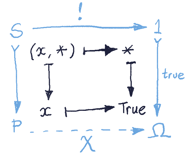
The fact that the two definitions coincide can be summarized by one commuting diagram. In the category of sets, given a characteristic function  , the subset and the monic are uniquely (up to isomorphism) defined as a pullback of this diagram.
We can now turn the tables and use this diagram to define the object called the subobject classifier, together with the monic  . We do it by means of a universal construction. We postulate that: For every monic
  between two arbitrary objects there exist a unique arrow
  such that the above diagram constitutes a pullback.
This is a slightly unusual definition. Normally we think of a pullback as defining the northwest part of the diagram given its southeast part. Here, we are solving a sudoku puzzle, trying to fill the southeast part to uniquely complete a pullback diagram.
Let’s see how this works for sets. To construct a pullback (a.k.a., a fibered product  ) we first create a set of pairs
  where
where  and
and  (the only element of the singleton set). But not all ‘s are acceptable, because we have a pullback condition, which says that
  , where
  is the element of pointed to by
  . This tells us that is isomorphic to the subset of for which is .
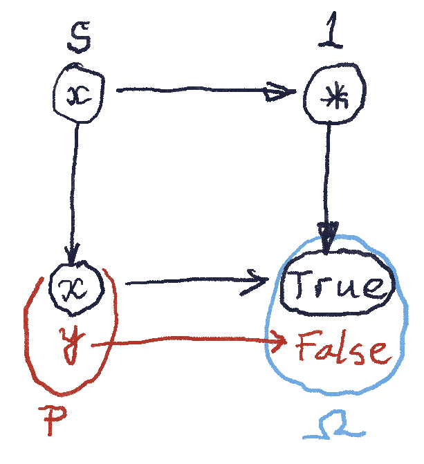
The question is: What happens to the other elements of ? They cannot be mapped to , so must contain at least one more element (in case is not an isomorphism). Can it contain more?
This is where the universal construction comes into play. Any monic (here, an injective function) must uniquely determine a that completes the pullback. In particular, we can pick to be a singleton set and to be a two-element set. We see that if contained only and nothing else, no would complete the pullback. And if contained more than two elements, there would be not one but at least two such ‘s. So, by the Goldilock principle, must have exactly two elements.
We’ll see later that this is not necessarily true in a more general category.
Next: Subfunctor Classifier.


Leave a comment